Article

Application of Soft Computing Models with Input Vectors of Snow Cover Area in Addition to Hydro-Climatic Data to Predict the Sediment Loads

by
Waqas Ul Hussan
1,*,
Muhammad Khurram Shahzad
2,*,
Frank Seidel
1 and
Franz Nestmann
1
1
Institute for Water and River Basin Management, Karlsruhe Institute of Technology (KIT), Kaiserstr. 12, 76131 Karlsruhe, Germany
2
Department of Civil Engineering and Technology, Institute of Southern Punjab, Multan 60000, Pakistan
*
Authors to whom correspondence should be addressed.
Water 2020, 12(5), 1481; https://doi.org/10.3390/w12051481
Submission received: 17 April 2020 / Revised: 18 May 2020 / Accepted: 18 May 2020 / Published: 22 May 2020
(This article belongs to the Section Hydrology)

Abstract

:
The accurate estimate of sediment load is important for management of the river ecosystem, designing of water infrastructures, and planning of reservoir operations. The direct measurement of sediment is the most credible method to estimate the sediments. However, this requires a lot of time and resources. Because of these two constraints, most often, it is not possible to continuously measure the daily sediments for most of the gauging sites. Nowadays, data-based sediment prediction models are famous for bridging the data gaps in the estimation of sediment loads. In data-driven sediment predictions models, the selection of input vectors is critical in determining the best structure of models for the accurate estimation of sediment yields. In this study, time series inputs of snow cover area, basin effective rainfall, mean basin average temperature, and mean basin evapotranspiration in addition to the flows were assessed for the prediction of sediment loads. The input vectors were assessed with artificial neural network (ANN), adaptive neuro-fuzzy logic inference system with grid partition (ANFIS-GP), adaptive neuro-fuzzy logic inference system with subtractive clustering (ANFIS-SC), adaptive neuro-fuzzy logic inference system with fuzzy c-means clustering (ANFIS-FCM), multiple adaptive regression splines (MARS), and sediment rating curve (SRC) models for the Gilgit River, the tributary of the Indus River in Pakistan. The comparison of different input vectors showed improvements in the prediction of sediments by using the snow cover area in addition to flows, effective rainfall, temperature, and evapotranspiration. Overall, the ANN model performed better than all other models. However, as regards sediment load peak time series, the sediment loads predicted using the ANN, ANFIS-FCM, and MARS models were found to be closer to the measured sediment loads. The ANFIS-FCM performed better in the estimation of peak sediment yields with a relative accuracy of 81.31% in comparison to the ANN and MARS models with 80.17% and 80.16% of relative accuracies, respectively. The developed multiple linear regression equation of all models show an R2 value of 0.85 and 0.74 during the training and testing period, respectively.

1. Introduction

Eroded sediment originating from drainage basins due to hydrometeorological processes like rainfall, snow melt, and ice melting, etc., is transported in the form of suspended loads and bed loads [1,2,3]. The bed loads are transported in the form of coarse particles of different shapes and sizes continuously in contact with the river bed [4]. The suspended load, transports in suspension state formed due to the erosion of fine particles from the sheet and gully, runoff in the catchment, river banks, and channel beds [5]. The increased runoff due to the rising rainfall, snow cover depletion, or glacier ablation, etc., often leads to an increase in flood events, increase in suspended sediments, channel bed erosion, pollutants in river ecosystem, and depletion of water storages, and damages or affects hydropower operations [6].
Sediment deposition in rivers and reservoirs is a very serious challenge worldwide. It leads to rapid depletion of water storage capacities which ultimately affects the supply of irrigation as well as power generation. It also affects the operation of water reservoirs to mitigate floods, polluting river ecosystem, and recreational sites [7,8]. In Asia, during the period 1990–2010 the net reservoir storages has been lost by 6.5% which is due to higher rate of sedimentations in the world [9]. In Pakistan, a number of water storages, for example the Tarbela, Mangla, Warsak, and Chashma storages, have lost considerable storage volumes earlier than expected [10,11,12,13] during the past three decades. The cause of this earlier-than-expected depletion of storages might be the high variance and incorrect estimation of sediment yields.
The Indus River in Pakistan with its total length of 2880 km supports the major storages and hydropower generations [14,15]. It is an economical source of hydropower generation having a 29% share in the country’s total national power generation capacity [16]. The Indus river has the world’s largest irrigation network, having an irrigated agricultural area of 181,000 km2 [16,17]. Hydropower projects generating more than 30,000 MW are planned on the Indus River for the future. Therefore, estimation of sediment yields for reaches in the Upper Indus Basin (UIB) is important for the design and operation of existing and new water infrastructures.
The erosion and transport of sediments are the outcome of complex physical processes. Their estimation is a difficult challenge due to the non-linearity of multiple factors controlling the sediment yield. Many factors including, among others, the amount of flows, sediment supplies, sources of sediments, catchment gully and channel erosion, river bed configuration, bed form resistance and slope, forces and moments controlling the incipient motion, and types and properties of sediment particles, control the amounts of sediments in rivers [18,19]. To overcome the challenges of sediment yield estimations, soft computing artificial intelligence methods have been developed over the past few decades. These soft computing machine learning techniques have replaced the traditional sediment rating curve (SRC), and multiple and auto-regressive models for estimation of sediment yields. The soft computing algorithms have proven a powerful tool for estimation of sediment yield from highly nonlinear processes of erosion and sediment transport.

Background

In the recent few decades, many researchers have used several black-box models for the prediction of sediment yield. The most widely used models among these black-box models include artificial neural networks (ANN), support vector machines (SVM), artificial neuro-fuzzy logic inference systems (ANFIS), and genetic programming (GP). Mostly, more than two models were used to compare the results for finding the best model for the prediction of sediment yields along with the rating curve (RC) model. For example, in some studies [20,21,22], ANN was found to be better for the prediction of sediment yields than the sediment rating curve (SRC) model. Similarly, ANN and multiple linear regression (MLR) models were used in some studies [23,24] for the estimation of sediment yields. In these studies, the sediment prediction results of ANN were found to be better than the sediment prediction results obtained by MLR. In yet another study [25], the grid rainfall and measured flows are used to predict sediment yields with ANNs by Levenberg-Marquardt (LM), scaled conjugated gradient (SCG), and Bayesian regulation (BR) algorithms. It was concluded that ANN with Levenberg-Marquardt algorithm performed fairly better than the other two ANN algorithms for sparsely distributed catchments with limited climatic recorded data. The results of ANN and ANFIS were compared by [26,27] for the prediction of sediment yield. In these studies, researchers found that ANFIS models show a higher accuracy than the ANN and SRC models. It was found in studies by [28,29] that gene expression algorithms are better than ANN and ANFIS models for predictions of sediment loads.
The studies [30,31] used the SVM along with ANFIS and ANN algorithms. The results obtained by SVM showed less erroring in comparison to those of the ANFIS and ANN models. The researchers referred to in [32] employed the ANN and SVM models using discharge and rainfall as input data to predict the sediment yields. They found that ANN is better than SVM for the prediction of sediments. The studies [33,34] used the wavelet artificial neural network (WANN) to compare their results with SRC, MLR, and ANN. They found that the WANN model is better than all other models used in the study. The study [35] used wavelet-based least-squares support vector machines (WLSSVM) along with WANN to compare the results for finding the better model for sediment predictions. The study revealed that WLSVM is more robust and better than WANN for estimation of sediment yields.
Heuristic regression models such as multiple adaptive regression splines (MARS), M5 decision tree regression learner, and support vector regression (SVR) have also been used in the recent decade for nonlinear modeling in water resources. In linear modeling, to capture the nonlinear behavior of the process involved in engineering specifically for flows and sediments, some improvements had been made by introducing methods like polynomial regression. In this regard, the multivariate regression spline (MARS) has been developed to detect the nonlinear relationship of inputs and outputs like discharge sediment yields [36,37]. MARS is a nonparametric regression model that identifies the desired pattern between inputs and desired output in the form of piecewise cubical or linear splines.
MARS, M5 model tree, and SVR are models used for the prediction of flows and sediment yields in water resources [38,39,40]. However, the use of MARS is comparatively rare for sediment yield predictions. The researchers referred to in [41,42] found that the performance of MARS is poor in comparison to that of dynamic evolving neural-fuzzy inference system (DENFIS) and ANN models. The study [43] compared the results of hybrid MARS fuzzy regression (HMARS-FR), fuzzy least squares regression (FLSR), and fuzzy least absolute regression (FLAR) for estimation of sediment yields. The hybrid MARS fuzzy regression was found to be better than the other two models for predictions of sediment loads. In another study [44] performed to predict sediment yields, the M5 model tree, SRC, GEP, and MLR models were used. The M5 model tree performed better than the SRC, GEP, and MLR models in this study. In yet another study [45] ANN, wavelet regression (WR), and M5 tree models were used for modeling the sediment yield using the inputs of flows and rainfall. In this study, the M5 model tree performed better than the ANN and wavelet regression models. Similarly, it was found in a study [46] carried out to predict sediments that the M5 tree model is better than ANN and fuzzy logic models. The study used hydro-climatic data for the predictions of sediments using five different algorithms namely, ANN Levenberg-Marquardt, ANN scaled conjugate gradient, SVR, M5 model tree, and REPTree model. In this study, the researchers found that ANN using the Levenberg-Marquardt algorithm performed better than other models. Table S1 in section of Supplementary Materials presents the summary of the literature discussed above.
The study presented in this paper checks the applicability of ANN Levenberg-Marquardt, hybrid ANFIS embedded grid partition (GP), hybrid ANFIS embedded subtractive clustering (SC), hybrid ANFIS embedded FCM clustering (FCM), and MARS models with inputs of grid climatic data, snow cover fraction, and flows to predict the sediment yields for sparsely distributed basins. These models were selected because, during the past three decades, the ANN and ANFIS data-driven models have been identified as being robust, powerful tools with a great ability of solving the complex nonlinear process-like prediction of sediment yields. As a result of the above discussions and scrutiny of literature review, and to the best knowledge of the authors, no study in artificial intelligence (AI) has used the combination of spatially averaged grid effective rainfall, mean basin-averaged temperature, and averaged basin snow cover fractions in combination with flows to predict the sediment yields.

2. Materials and Methods

2.1. Study Area

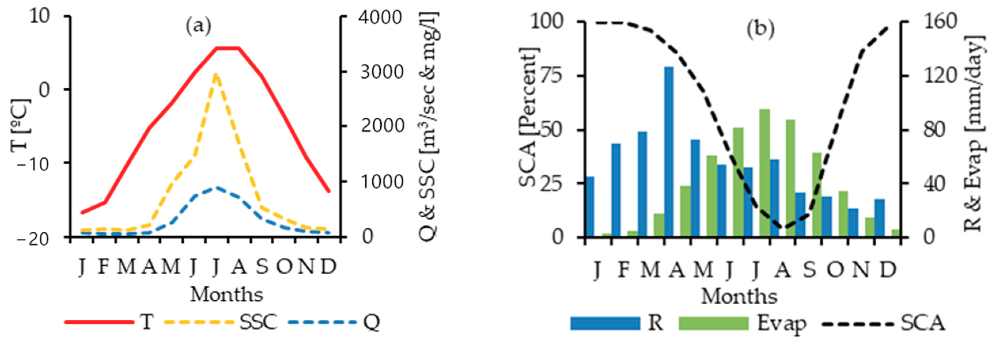
The present study was carried out in the Gilgit River basin situated in the Hindukush Mountains of the Upper Indus Basin (UIB). The Gilgit River originates from Shandoor Lake north of the Gilgit-Baltistan region in Pakistan. The Baha Lake is the right tributary of the Gilgit River with small tributaries being e.g., Yasin, Ishkoman, and Phandar. The Phandar Lake is located in Ghizer. The Yasin tributary joins the main Giglit River near Gupis. Figure 1 and Figure 2 show the hydrological characteristics of the Gilgit basin that has a drainage area of 12,095 km2. The geographical location of the Gilgit basin is between latitude 35°55′35 N and 36°52′20″ N and longitude 72°26′04″ E and 74°18′25 E. The elevation of catchment ranges from 1454–7048 m a.s.l. Table S2 in supplementary materials shows the key features of the Gilgit basin. About 10% of the total catchment area is covered with glaciers and lies above an elevation of 5000 m. During the winter season, approximately 87% of the catchment area is covered with snow cover which reduces to 11% during the ablation period in summer. The mean annual discharge and suspended sediment concentrations (SSC) of the Gilgit basin are 291 m3/sec and 448 mg/L, respectively. The ablation period starts in July after seasonal snow melts. The melting of the glacier is slow and continues until the month of October. Then, the accumulation period of snow starts at the end of October. The Gilgit basin receives 75% of its rainfall starting from the mid of spring (April) to the end of summer (October). The mean annual basin rainfall from grid data in the Gilgit basin is approximately 670 mm. The mean monthly basin average temperature for the Gilgit basin ranges from −19.8 to 7.20 °C.
The Water and Development Authority (WAPDA) of Pakistan had also installed stream gauging stations at an altitude of 1430 m a.m. sea level for measuring flows and suspended sediment concentrations (SSC). The climatic stations installed in the Gilgit basin are sparsely distributed in the catchment. The climatic stations installed in the valley by the Pakistan Meteorological Department (PMD) at Gilgit and Gupis have at their disposal long-term daily climatic data collected from 1981–2010. However, the climatic stations of Uskhkore, Yasin, and Shendure located on higher altitudes are sparsely distributed and have short-term recorded data accumulated from 1996–2010 which are available from WAPDA. However, the suspended sediment concentrations (SSC) are recorded on intermittent days per week. Table 1 shows the detailed information on the data used in this study. The flows, temperature, and rainfall are recorded on a daily basis. Because of the scarcity of climatic information and the sparse distribution of climatic stations in the Gilgit catchment (see Figure 1 and Figure 2), the information of grid climatic, snow cover fractions, and grid evapotranspiration datasets of Table 1 were used for the period 1981–2010 during analysis of this research work. These grid datasets were extracted using the Shuttle Radar Topography Mission’s (SRTM) Digital elevation model (DEM) of 30 m for Gilgit catchment.
The Moderate Resolution Imaging Spectroradiometer (MODIS) MOD10A2 product was downloaded on a weekly basis for the period of 2000–2010 from the National Snow and Ice Data Center (NSIDC) online server. The MODIS data with 500 m resolution was used for estimating the snow cover area and snow melt runoff [49,50]. The same procedure was adopted in other studies to estimate and linearly interpolate the snow cover fractions for daily snow cover fractions of the Gilgit basin for the period of 2000–2010 [49,50]. The temperature-index snow model was further used to estimate the snow cover fraction for the period of 1981–2010 after calibration and validation of the snow model with MODIS snow cover.
Table 2 shows the Pearson’s correlations of input variables used in this study. Generally, correlation analysis such as cross correlation, auto-correlation, and partial auto-correlation are also used to determine the input combinations of various variables with lag times. However, the main deficiency of these methods is the inability to cover the nonlinear relationship between the input and output variables like discharge sediment, etc. For this reason, in the current study, the various input combinations were identified by examining the test accuracy of the model output.
In general, the discharges trigger the channel erosion. However, in addition to discharges, the temperature and snow cover area of the snow- and ice-dominated basin also triggers hillslope erosion, snow melt erosion and glacier melt erosion. The evapotranspiration also has an indirect relationship with erosion processes in the form of the vegetative cover of the plants and forests. Keeping in view the importance of direct and indirect factors controlling the erosion of catchments, different variables other than discharges such as snow cover area, effective rainfall, and evapotranspiration were also chosen in this study for the prediction of sediment yields. Prior to the analysis for prediction of sediment yields, the flows and suspended sediment load (SSL) were transferred into a log transformation form to compensate the biases and very high values in datasets. The datasets were divided into 70% and 30% for training and testing of the model, respectively. Shahin et al. [51] suggested that for optimum performance of soft computing methods datasets should be divided into training (i.e., 70%) and testing (i.e., 30%) phases. The daily datasets of measured SSC were not available for continuous days. The measured SSC values were available for total 767 days during the period 1981–2010. For the sediment rating curve (SRC) the flows and SSC values for the period 1981–2003 (i.e., 1–537 days) and 2003–2010 (i.e., 538–6767 days) were used for training and testing respectively. However, the random sampling [52] of whole datasets for training (70%) and remainder datasets as testing (30%) were conducted in MATLAB to reduce over and under fitting of network. Then ANN, ANFIS, and MARS models were trained and tested in MATLAB with various input combinations.

2.2. Application of Temperature-Index Snow Model for Snow Cover Estimates

The climatic stations in the Gilgit basin have less availability of long-term climatic records for the catchment. Previous studies [53,54,55] reported that the rainfall on higher elevations starting above 5000 m in the Upper Indus Basin (UIB) is 5–10 times higher than the rainfall recorded in the valley. For this reason, the grid data for rainfall and temperature from the HI-AWARE project [47,48] was used in this study. Keeping in view the above-mentioned constraints, the temperature-index snow model is used in this study. The temperature-index snow model is a simple and spatially distributed model which, in addition, has less data requirements. In this study, this method is used to simulate the long-term snow melts and snow cover fractions after calibration and validation of the simulated snow cover fraction with the MODIS snow cover fractions for the period of 2000–2010.
In the temp-index snow melt model [56,57], precipitation P is first separated into snow and liquid rain on a daily time scale. The threshold temperature TRS (°C), daily maximum temperature (°C), and daily minimum temperature (°C) separate the snow and liquid rainfall as:
{ R a i n = R = C p P   S n o w = S = ( 1 C p ) P
where,
Precipitation factor Cp proportionate to temperature difference is calculated as:
{ C p = 1   i f   T m i n > T R S   C p = 0   i f   T m a x T R S   C p = T m a x T R S T m a x T m i n   i f   T m i n T R S < T m a x
The threshold temperature TRS is used to define the type of precipitation into rain/snow and the threshold temperature TSM for the snow melt process which depends on numerous factors like the boundary layer condition of atmosphere, temperature, and air humidity, etc.
Then, daily rates of snow melt, i.e., Msnow (mm/day) are estimated as:
{ M s n o w = K s n o w ( T m e a n T S M )   i f   T m e a n > T S M   M s n o w = 0   i f   T m e a n > T S M  
Here, the Ksnow (mm/day °C) is the degree day factor for snow melts, Tmean (°C) is the mean daily air temperature, and TSM (°C) is the threshold temperature.
After this, the snow model simulates the snow water equivalent or snow depth SD (mm) for each grid number of i as:
S D i ( t ) = S D i ( t 1 ) + S i ( t ) M s n o w i ( t )
Finally, the snow cover fraction SCF for i = 1, 2, 3, 4,…, N number of grids for the whole basin is estimated for calibration and validation with the MODIS snow cover fraction as:
S C F   ( t ) = 1 N i = 1 N H   [ S D i ( t ) ]
Here, H = unit step function; when H = 0, SD = 0 and H = 1 then SD > 0. The area of integration N is the entire basin, sub-basins, and elevation bands, etc.

2.3. Artificial Neural Networks (ANN)

Artificial neural networks (ANNs) are data-based black box models primarily inspired by the concept of functioning of the biological nervous system. ANNs consist of a set of processing elements referred to as neurons. These neurons work in the parallel systems for acquiring the information and storing the knowledge for computational use. ANNs consist of three layers as their basic structure. These layers are the input layer, the hidden layer (processed layer), and the output layer. Each layer is connected by networks of neurons with preceding layers. This system of networks connected with neurons is called multilayer perceptron (MLP). There are various types of ANNs that perform various assignments in science and engineering. Among these ANNs of MLP, feed-forward back propagation FFBP-ANN is most popular. The literature [58,59,60,61,62,63,64] explains the details of the ANN model and its application to water resources with FFBP-MLP algorithm. In FFBP-MLP, the input data are learned in forward direction of network from input nodes to the hidden nodes with some transfer functions in the hidden layer. Then, the information is forwarded from the hidden layer to the output nodes. Figure S1 in supplementary materials explains the architectures of the FFBP ANN. In the output layer, an output is generated by the network, and the error between predicted and model output is computed. This output error of the network is back-propagated through the network to correct the connection weights of neurons in the hidden layer. This learning process of the network is performed until the minimum error is optimized to avoid overfitting as well underfitting of the network.
A neural network is described with (1) architectures of layers connected with networks of neurons, (2) transfer functions, and (3) training methods for estimation of weights in nodes. In general, the performance of ANN depends on its model network, learning complexity, and problem complexity. The performance of ANN depends on the number of neurons in hidden layers and the number of hidden layers to avoid the over- and underfittings of the network. The literature suggests the optimum neurons to be in the range of 2 N 1 + N 0 , where N1 and N0 are the number of input and output neurons, respectively.
For this study, ANN with FFNN-MLP with Levenberg-Marquardt has been used with one hidden layer as more than one hidden layer increases the complexity of the network and does not improve the results, either. The FFNN-MLP with Levenberg-Marquardt is a robust and powerful tool. It has a high and fast ability of data convergence, and produces more accurate results than other ANN algorithms.

2.4. Adaptive Neuro-Fuzzy Logic Inference System (ANFIS)

The adaptive neuro-fuzzy logic inference system (ANFIS) is a novel architecture with combinations of neural networks and fuzzy inference systems (FIS). A basic ANFIS [65] structure is shown in Figure S2 in section of supplementary materials. The ANFIS works by tuning the parameters of FIS applying the neural network learning method. The ANFIS builds a network structure connected with a number of nodes. These nodes are characterized by fixed or adjustable parameters. The ANFIS uses neural networks with fuzzy logic if-then rules with appropriate membership functions to translate the input parameters into output values. Three inference systems are classified as Tsukamoto’s, Mamdani’s, and Sugenos’s systems. The Mamdani’s system [66] was mostly used in the past. The Sugeno’s system [67] is more efficient than other systems. In this study, Sugeno’s fuzzy logic structures were used.
As an example, it is assumed that a FIS has two inputs x1 and x2 with target values of z. Here, input of discharge and snow cover can be supposed as x1 and x2 with output z as sediment yield for a particular time t. Then, in Sugeno’s fuzzy logic structures, typical rule sets with two IF/THEN rules are expressed as:
Rule   1 :   IF   x 1   is   A 1   and   x 2   is   B 1 ,   THEN   z 1 = f 1 = p 1   x 1 + q 1   x 2 + r 1
Rule 2 :   IF   x 1   is   A 2   and   x 2   is   B 2 ,   THEN   z 2 = f 2 = p 2   x 1 + q 2   x 2 + r 2
where pi, qi, and ri are parameters corresponding to Rule 1, Rule 2… Rule n.
The ANFIS consist of five layers.
Layer 1: In the first layer, each node generates a membership grade for the variable of each input. The output of ith node with generalized bell membership function in the first layer is expressed as:
O i 1 = μ   A i ( x 1 ) = 1 1 + ( ( x 1 c i ) ) a i ) 2 N i
where, {ai, ci, Ni} are the parameter sets for x1 input in ith node. These parameters change the shape of the bell function in the range of 0–1.
Layer 2: Layer 2 is labeled with II in each node. In this layer, each node multiplies the incoming signals coming from layer 1 as:
O i 2 = w i = μ   A i ( x 1 ) × μ   B i ( x 2 ) ,     i = 1 ,   2
Layer 3: In layer 3, each node calculates the normalized firing strength as its relationship between firing strength of ith rule to the sum of all rules:
O i 3 = w ¯ = w w 1 + w 2     i = 1 ,   2
Layer 4: In layer 4, the sums of signals from second- and third-layer networks are calculated for each ith node toward the model output as:
O i 4 = w ¯ i f i = w ¯ i ( p i   x 1 + q i   x 2 + r i ) i = 1 ,   2
Here, w ¯ is the output from layer 3 in this equation.
Layer 5: Layer 5 calculates the overall output in the form of a single node as the ANFIS model output against each target value as:
O i 5 = Σ w ¯ i f i = Σ w ¯ i f i Σ w ¯ i     i = 1 ,   2
In the ANFIS model, to obtain the model parameters, a hybrid learning method is used for this study. Further details about the ANFIS model can be found in [68].
In this study, three strategies are used to produce the initial fuzzy inference system for the ANFIS model. These strategies are grid partition (ANFIS-GP), subtractive clustering (ANFIS-SC), and fuzzy c-means clustering (ANFIS-FCM). The ANFIS-GP is a combination of ANFIS and grid partition. In grid partition, the input linguistic variables are partitioned by fuzzy numbers and their membership functions (MFs). The grid partition uses predefined numbers of MFs to optimize the MFs according to input–output datasets. The quantitative characteristics of datasets are separated into n partitions (n = 2, 3, 4…). In this study, eight MFs were used, such as gaussmf, gauss2mf, trimf, trapmf, gbellmf, pimf, dsig, mf, and psigmf. In the AFNIS-GP model, the number of rules increases exponentially with the increase in the number of input variables. For details about the ANFIS-GP, see [65].
The ANFIS-SC model is the extended model derived from the mountain clustering model [69] with combination of the ANFIS model by using the subtractive clustering strategy. This model was modified by Chiu [70]. This method has an advantage over the mountain clustering method. It eliminates the grid resolution to reduce the complex computations in the mountain clustering method. In the ANFIS-SC model, each dataset is considered as potential cluster. Then, the potential of each data point of a given dataset is calculated by its distance from all other data points. These data points having many neighboring data points show a high potential value. The influential radius decides the number of clusters in the ANFIS-SC model. The small value of influential radius has many numbers of clusters with more rules in comparison to its large value [71]. Using a hit-and-trial procedure, the suitable critical value of influential radius is sorted out during the data space clustering procedure. [70,72] further explain the detailed procedure of the ANFIS-SC model.
The ANFIS-FCM model was proposed in the literature [73,74,75,76,77] and enhanced by Zhang and Chen [78]. The ANFIS-FCM minimizes the errors by partitioning the X datasets into C clusters. This method reduces the errors regarding the weighted distance of each data point xi toward all centroids of the C clusters. After this, the ANFIS-FCM model minimizes the objective function as:
M i n   J F C M = c = 1 C i = 1 N w p i c x i v c 2   s . t .   c = 1 C   w i c = 1 ,   i = 1 ,   2 ,   ,   N
where C, N, wic, v, and x are the number of clusters, number of data points, degree belongs to ith data point of Cith clusters data points, and input data sets. The p (p > 1) entitles to the fuzzifier exponent. In ANFIS-FCM, wic is calculated as:
w i c   = 1 i = 1 c ( d i c 2 d i j 2 ) 1 ( p 1 )   f o r   i = 1 ,   2 , N   a n d   c = 1 , 2 , C
In the FCM model after initialization of the center vectors, centers are recomputed as:
v c   = j = 1 N w p J c   x j j = 1 N w p J c   f o r   c = 1 ,   2 , N   a n d   1 p N
The algorithm is run until the convergence condition is completed.

2.5. Multivariate Adaptive Regression Splines (MARS)

MARS is a non-parametric technique for the prediction of nonlinear processes developed in 1991 by Friedman [79]. The MARS model is a flexible and precise prediction model. It has been successfully applied in different studies [80,81,82] for prediction and forecasting purposes. In the MARS model, the MARS function develops a series of linear segments having different slopes from the input–output relationships of given datasets. Each linear segment of MARS is then fitted with a linear basis function. For this study, the datasets were separated into break values between different regions or segments referred to as knots. Each region has its own regressions line. The shape of a piecewise linear basis function is expressed as:
[ max   ( 0 , x k ) ]   O R   [ max   ( 0 , k x ) ]  
Here, x represents the predictor variable and k explains about the threshold value of the knots. In general, MARS consists of combinations of basis functions (BFs) given as:
y = f ( x ) + ε
f ( x ) = β o + β m B F m ( x )
In the above Equation (12), the variable y is dependent on the estimated values of function f(x) with the error ε . In Equation (13), β o is a constant value, B F m is the basis function, and β m represents the coefficient for the maximum number of basis functions (BFs) depending on the input’s datasets.
In the MARS model with polynomial knots, there exist two phases called forward step phase and backward step phase. The forward step phase generates all possible BFs. After generation of the BFs, the generalized cross validation criterion (GCV) is used for determining the BFs and appropriate nodes. After this forward step phase, the backward step phase of the MARS model works to reduce the number of BFs for improving the predictions and avoiding overfitting of the model. [79] gives detailed information about the MARS model.

2.6. Sediment Rating Curve (SRC)

The sediment rating curve is an empirical relationship of flows and sediment load or concentrations described as:
S S L ( t ) = a × Q b ( t )
where Q (m3/day) is discharge, SSL (tons/day) both in log transformation form, and a and b are the constants that depend on the characteristics of a river and its catchments.

2.7. Performance Measurement Metrics for Model Evaluation

The performance of models was measured and assed using the following statistics:
Root-mean-square error (RMSE):
R M S E = 1 N   i = 1 N ( ( S i o ) ( S i s ) )   2  
Nash–Sutcliffe efficiency (NSE):
N S E = 1 t = 1 N ( S i o S i s ) 2   t = 1 N ( S i s S i s ¯ ) 2     N S E 1
Pearson’s correlation coefficient (R2):
R 2   = ( i = 1 N ( S i 0 S i o ¯ ) ( S i s S i s ¯ ) i = 1 N ( S i 0 S i o ¯ ) 2 i = 1 N ( S i s S i s ¯ ) 2 ) 2
where N refers to the data quantity, Sio is the observed sediment, Sis is the simulated sediments, and S i s ¯ is the mean of the simulated sediments.
Relative accuracy:
The relative accuracy is the %age of accuracy expressed as:
Relative   Accuracy   ( % age ) = ( 1 | S p o S p s S p o | ) × 100
where Spo is the observed peak value of SSY, Sps is the simulated peak value of SSY.

2.8. Application of the ANN, ANFIS-GP, ANFIS-SC, ANFIS-FCM, and MARS Models

For application of the ANN, ANFIS-GP, ANFIS-SC, ANFIS-FCM, and MARS models various input combinations with daily lag time were examined with scenarios starting from S1–S15 by testing the accuracy of the network using minimum RMSE and maximum values of R2 and NSE as performance criteria. The input scenarios developed in this study for predictions of sediment yields are listed here:
(a)
Flows
S1 = SSCt = f (Qt, β1) + ei
S2 = SSCt = f (Qt, Qt−1, β1, β2) + ei
S3 = SSCt = f (Qt, Qt−1, Qt−2, β1, β2, β3) + ei
S4 = SSCt = f (Qt, Qt−1, Qt−2, Qt−3, β1, β2, β3, β4) + ei
S5 = SSCt = f (Qt, Qt−1, Qt−2, Qt−3, Qt−4, β1, β2, β3, β4, β5) + ei
(b)
Flows and snow cover area
S6 = SSCt = f (Qt, SCAt, β1, β6) + ei
S7 = SSCt = f (Qt, SCAt, SCAt−1, β1, β6, β7) + ei
S8 = SSCt = f (Qt, SCAt, SCAt−1, SCAt−2, β1, β6, β7, β8) + ei
(c)
Flow, snow cover area, and effective rainfall
S9 = SSCt = f (Qt, Rt−1, SCAt, SCAt−4, β1, β9, β6, β10) + ei
(d)
Flow, snow cover area, temperature, and evapotranspiration
S10 = SSCt = f (Qt, Tt−1, Evapt−1, SCAt, SCAt−4, β1, β11, β12, β6, β10) + ei
(e)
Average mean basin air temperature
S11 = SSCt = f (Tt, β13) + ei
S12 = SSCt = f (Tt, Tt−1, β13, β11) + ei
S13 = SSCt = f (Tt, Tt−1, Tt−2, β13, β11, β14) + ei
S14 = SSCt = f (Tt, Tt−1, Tt−2, Tt−3, β13, β11, β14, β15) + ei
S15 = SSCt = f (Tt, Tt−1, Tt−2, Tt−3, Tt−4, β13, β11, β14, β15, β16) + ei
In the combinations above, β1–β16 represent the membership functions of layers in the ANN, ANFIS, and MARS models.

3. Results and Discussion

3.1. Simulation of Snow Melts and Snow Cover Area

The results of the calibrated temperature-index snow melt model are shown in Table 3. The model was calibrated and validated to simulate the snow cover by using the degree day factor for the snow model. Table 3 shows the value of the degree day factor ksnow = 4.2 (mm/day/°C) for the Gilgit basin. The literature review [49,50,83,84,85,86] for the regional case studies shows that the value of Ksnow ranges from 3–7 (mm/day/°C) in the Upper Indus Basin (UIB). Thus, during calibration and validation of the temperature-index snow model for this study, the value of ksnow = 4.2 (mm/day/°C) lies within the range of the values of previous studies carried out for snow melt runoff modeling in the UIB. The difference between the Ksnow value in the current study and that of previous studies is probably due to the use of different resolutions of input datasets, lengths of calibration datasets, threshold temperatures for separating rainfall and snow, threshold temperatures for snow melts, and characteristics of the catchment.
Table 3 also shows the performance measurement statistics for the snow model during the calibration and validation periods. The value of R2 is found at 0.90 between the MODIS-observed snow covered area and model simulated snow cover area both during the calibration and validation periods. The performance evaluation criteria using the three criteria of R2, NSE, and RMSE show that goodness of fit between the model and observed MODIS snow cover maps is more than 70% which is satisfactory in estimation of both the snow melts and snow cover area. Figure 3 also shows the time series plot between model snow cover area and MODIS-observed snow cover area during the calibration (2000–2007) and validation (2008–2010) period, respectively.
For application of the ANN model, the transfer functions logsig, purelin, tansig, and radbas were used in the hidden layers. The network was trained by using 16 combinations of four transfer functions for input and output layers. The optimum number of neurons was determined ranging from 3–8 in single hidden layers for overall input scenarios giving best results at the end. Table 4 shows the results of various input combinations using ANN model. For the ANFIS-GP, ANFIS-SC, and ANFIS-FCM models, the hybrid algorithm was used in this study.
For the ANFIS-GP model application, the gaussmf, gauss2mf, trimf, trapmf, gbellmf, pimf, dsigmf, and psigmf membership functions were used. In ANFIS-GP, the type of membership functions and number of member functions are important for training the network. Table 5 shows the results of all scenarios using the ANFIS-GP model with optimal number and type of membership functions. The optimal number of functions ranges between 2 and 4 for all scenarios.
For application of the ANFIS-SC model, the network is trained with an optimal range of the radius of clusters which give a minimum value of RMSE and highest values of R2 and NSE. The optimal value of the cluster radius represents the influence of the cluster radius on the dataset clusters. If the cluster radius is small, then there are numerous small cluster datasets.
On the other hand, a large value of the cluster radius means that there are a few large cluster datasets for training the network. During training of the network, the hit-and-trial method was used to find out the optimum value of the cluster radius with the smallest value of RMSE for all scenarios during the testing period. Table 6 shows the results of the ANFIS-SC model for all scenarios. It was found that the optimal range of the cluster radius is from 0.5–0.9 for all scenarios.
For application of the ANFIS-FCM model, the various numbers of clusters were used to train and test the network for all scenarios. Table 7 shows the results of the ANFIS-FCM model for all input combinations. The optimal number of clusters ranges between 2 and 6 for this study with the lowest value of RMSE and highest value of R2 during testing of the network for all input combinations.
For application of the MARS model, the controlling parameters generally include the maximum basis functions, maximum interaction, speed factor, minimum number of observations between knots, penalty of variable, and degree of freedom. However, for this study, the hit-and-trial method was used to train the model with an optimal number of maximum basis functions ranging from 5 to 25 for all input scenarios with the remaining parameters being default values in the model. Table 8 shows the results of the MARS model for various input scenarios used in this study.
For application of the sediment rating curve (SRC) model, the power law function was used to train the model with 70% of the datasets after transformation of flows and sediment yields into logarithm form.
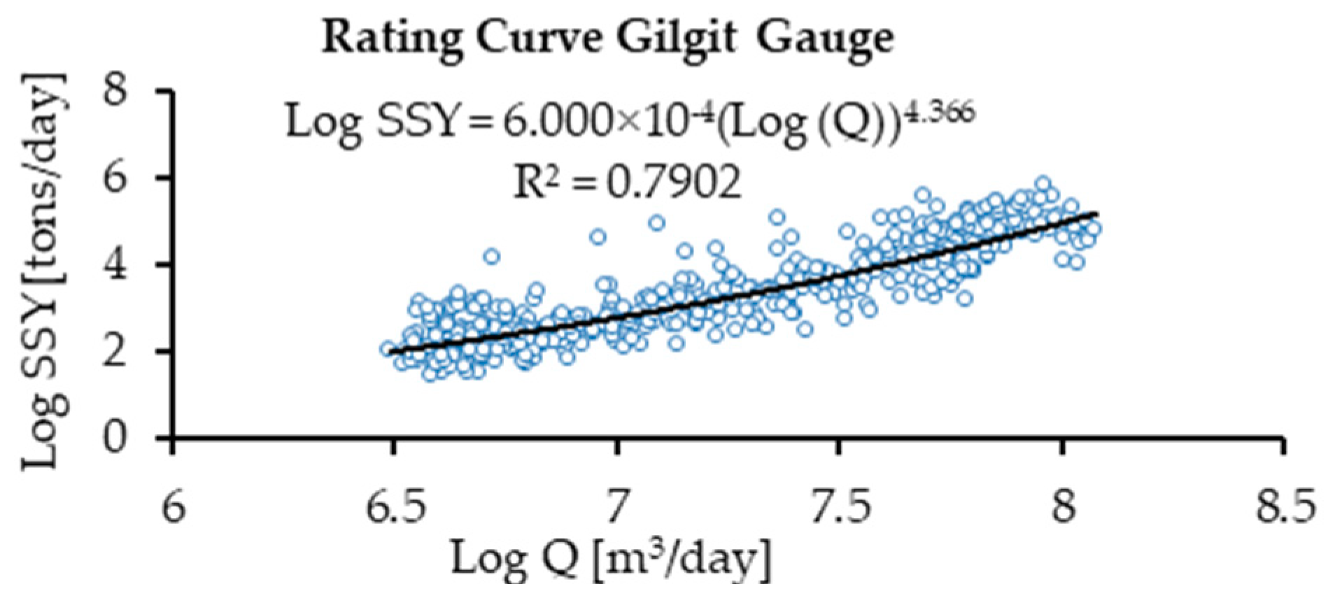
After training of SRC with 70% of the data sets, the model was tested with 30% of the remaining data. Figure 4 shows the plot of the sediment rating curve using the power law functions. Table 9 also shows the results of training and testing of the sediment rating curve (SRC) model and compares its model performance statistics with other models used for predictions of sediment yields used in this study.

3.2. Comparison of the ANN, ANFIS-GP, ANFIS-SC, ANFIS-FCM, MARS, and SRC Models

The results of the training and validation of the various scenarios are shown in Table 4, Table 5, Table 6, Table 7, Table 8 and Table 9 for the ANN, ANFIS-GP, ANFIS-SC, ANFIS-FCM, MARS, and SRC models for predictions of the sediment yields for the Gilgit basin. In Table 4, the ANN shows the best performance of S10 scenarios with model inputs of Qt, Tt−1, Evapt−1, SCAt, and SCAt−4. In the ANN, the model parameters having radbas and tansig as input and output transfer functions along with five numbers of neurons performed best with S10 input scenarios during the training and validation phases. Table 5 shows the results of the ANFIS-GP for all input scenarios. Here, the ANFIS-GP shows the best performance of the model with S7 scenarios consisting of inputs of Qt, SCAt, and SCAt−1. The ANFIS-GP model performs best with model parameters consisting of triangular (trimf) membership functions along with two numbers of membership functions (MFs). The results of the ANFIS-SC model are shown in Table 6.
From Table 6, the input scenario S10 involving the inputs of Qt, Tt−1, Evapt−1, SCAt, and SCAt−4 gives the best performance of the ANFIS-SC model. The ANFIS-SC uses the model parameters having the value of a cluster radius of 0.90 to perform best with S10 input combinations. Table 7 shows the results of input scenarios by using the ANFIS-FCM model. It is evident that the best performance of the ANFIS-FCM model, too, was obtained with S10 scenarios having inputs of Qt, Tt−1, Evapt−1, SCAt, and SCAt−4. In the ANFIS-FCM model, the best network was developed by using the model parameter having two numbers of clusters with S10 input scenario.
Table 8 represents the results of the MARS model used in this study for prediction of the sediment yield of the Gilgit River basin. As shown in Table 8, again the input scenario S10 involving the inputs of Qt, Tt−1, Evapt−1, SCAt, and SCAt−4 developed the best-performing network in the MARS model. The MARS model performed best with its basis function (BF) parameter having the value of 10 with the S10 scenario.
Table 9 shows the overall results of the best networks of the ANN, ANFIS-GP, ANFIS-SC, ANFIS-FCM, and MARS models compared with the sediment rating curve performance for the Gilgit basin. Table 8 shows that the ANN model performs better than all other models with the least values of the RMSE errors of 0.42 and 0.43 during the training and testing phase.
Similarly, Figure 5 shows the scatter plot between the observed and predicted SSY by using ANN, ANFIS-GP, ANFIS-SC, ANFIS-FCM, MARS, and SRC during the testing phase for overall best input scenarios. From the scatter plot graphs, it can be observed that the ANN-based model has the least scatters with the highest value of R2 during the testing phase. The ANN has improved the results of the scatter plot of the R2 value to up to 0.82 in comparison to the rating curve R2 value of 0.71 during the testing period.
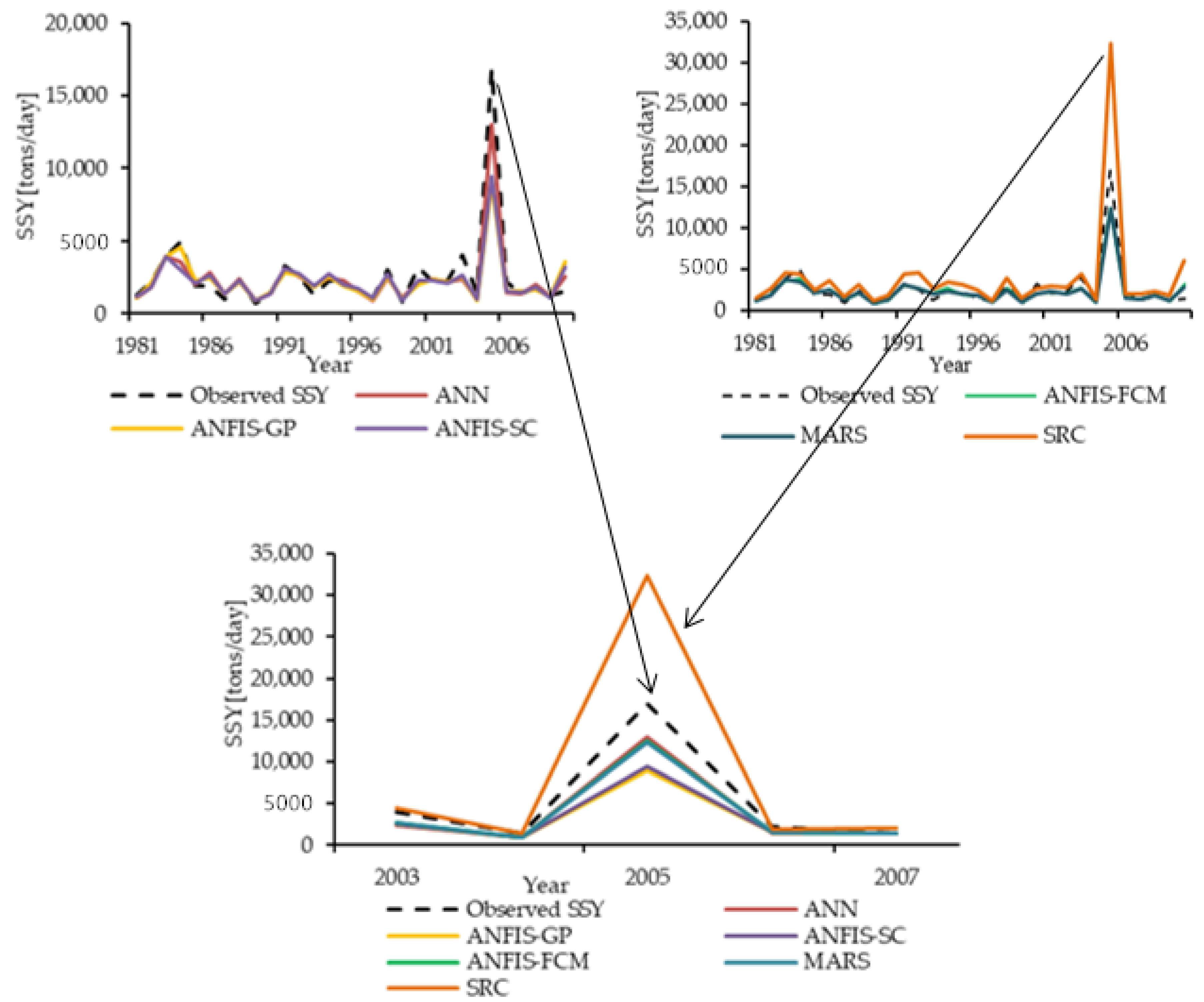
Figure 6 shows the annual time series variation graphs of the observed and estimated SSY by using the ANN, ANFIS-GP, ANFIS-SC, ANFIS-FCM, MARS, and SRC models with best- performed input combinations. This Figure 6 also includes the one detailed graph derived from the main time series plot to compare all model performances during the peak annual suspended sediment yields (SSY) period of the year 2005.
It is illustrated in Figure 6 that during the peak SSY period of the year 2005, the estimated SSY of the models ANN, MARS, and ANFIS-FCM are relatively closer to the observed SSY than those of the other models. However, the models ANFIS-GP and ANFIS-SC significantly underestimated the SSY during this peak year period of 2005. Similarly, the SRC model significantly overestimated the SSY during that period.
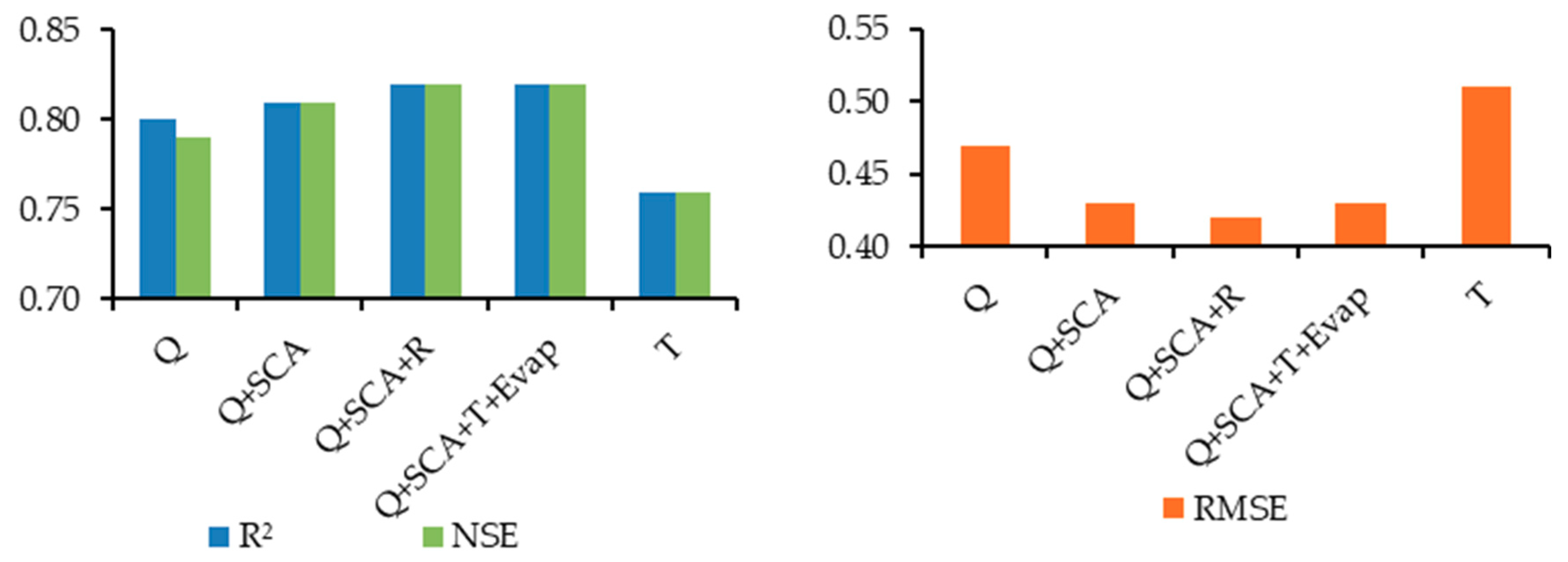
Figure 7 shows an overall comparison of different input variable scenarios developed from flows Q (m3/day), snow cover area SCA (fractions), effective mean basin rainfall R (mm/day), mean basin average temperatures T (°C/day), and mean basin evapotranspiration Evap (mm/day) for predictions of SSY during the testing period in the Gilgit basin. The model performance of R2 was improved up to the value of 0.82 by introducing the combinations of the snow cover area along with flows, effective rainfall, temperatures, and evapotranspiration. The input combinations consisting of only the mean basin average temperature T perform less than other combinations consisting of flows, snow covers, effective rainfall etc. However, the mean basin average temperature T variable scenarios’ performance with an R2 value of 0.76 is better than the rating curve with an R2 value of 0.71.
Rajaee et al. [22] applied artificial neural networks (ANNs), neuro-fuzzy (NF), multiple linear regression (MLR), and sediment rating curve (SRC) for prediction of suspended sediment concentrations (SSC) for Little Black River and Salt River in United states of America (USA). For example, in Little Black River gauging station, the value of R2 was 0.69 for NF model, while it was 0.45, 0.25, and 0.23 for ANN, MLR, and SRC models respectively. In the present study, the value of R2 ranges from 0.78–0.82 using ANN and ANFIS models. It suggests that the soft computing models could be successfully applied for daily prediction sediment yields.
The mean values of SSY and relative accuracies of the ANFIS-GP, ANFIS-SC, ANFIS-SC, ANFIS-FCM, MARS, and SRC models at Gilgit gauging station are shown in Table 10. The ANN model predicted the means of the peak sediment fluxes to be 6613 (tons/day) and 5186 (tons/day), while the ANFIS-GP, ANFIS-SC, ANFIS-FCM, MARS, and SRC models resulted in less accurate outcomes. However, Table 10 also shows that the ANFIS-FCM model with a relative accuracy of 81.31% has a superior accuracy in predicting the peak values of sediment yields compared to the ANN (80.17%), ANFIS-GP (78.45%), ANFIS-SC (75.49%), MARS (80.16%), and SRC (66.33%) models.

3.3. Deveoplement of Multiple Linear Regression Equation

The relationships between the measured sediment yields and the best-performing scenarios of the ANN, ANFIS-GP, ANFIS-SC, ANFIS-FCM, and MARS models have been developed using 70% of the data. The remaining 30% of the data was used to test the equation of multiple linear regression developed between the measured sediments and data-based model outputs. Equation (24) represents the relation between log-transferred measured sediments loads and data-based log-transferred modeled sediment loads as:
y   = 0.60 x 1 + 0.45 x 2 + 0.11 x 3 + 0.20 x 4 0.05 x 5 0.19 x 6 0.39
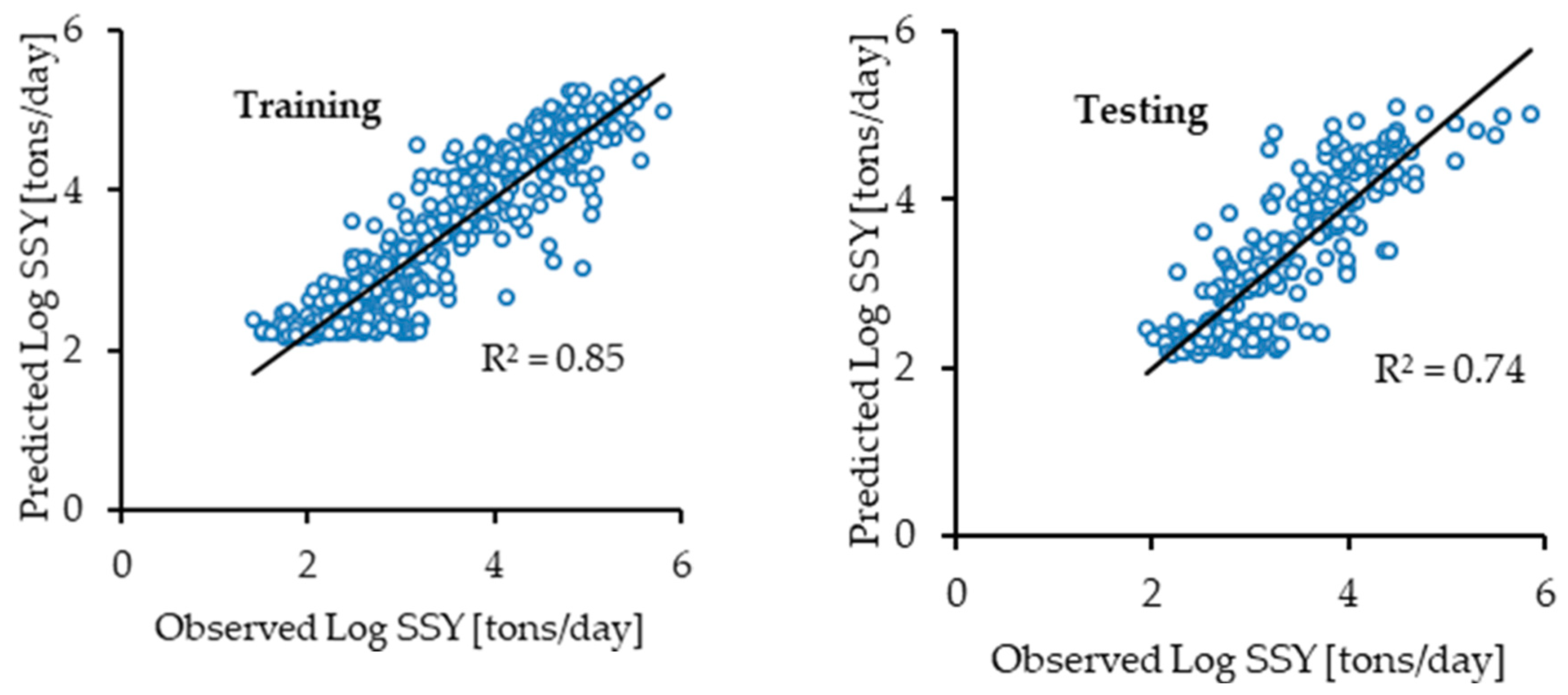
where y = observed/measured sediment load in log form (tons/day), x1 = ANN model outputs of sediment load in log form (tons/day), x2 = ANFIS-GP model outputs of sediment load in log form (tons/day), x3 = ANFIS-SC model outputs of sediment load in log form (tons/day), x4 = ANFIS-FCM model outputs of sediment load in log form (tons/day), x5 = MARS model outputs of sediment load in log form (tons/day), and x6 = SRC model outputs of sediment load in log form (tons/day). Figure 8 shows the results of the multiple linear regression Equation (23) during the training and testing periods.

4. Conclusions

This study was designed to improve the predictions of sediment yields by using different input variables applying the ANN, ANFIS-GP, ANFIS-SC, ANFIS-FCM, and MARS models in addition to the SRC model to the snow- and ice melt-dominated Gilgit basin. The objective of the study was to compare and examine the appropriate input variables based on the knowledge of hydrological process- and snow- and ice melt-dominated factors controlling erosion and sediment transport for predictions of sediment yields. To accomplish this objective, we investigated the input such as flows affecting channel erosion; temperature and snow cover area as snow melt erosion, glacier melt erosion and hillslope erosions; effective rainfall as mass wasting erosion, hillslope erosions and channel erosion; and evapotranspiration as effect of vegetation cover controlling catchment erosion for the prediction of sediment yields. It was concluded that for the prediction of sediment yields, the inputs of snow cover area, effective rainfall, and evapotranspiration significantly improve the accuracy of the ANN model when used in addition to flows and temperature as inputs. Combining the snow cover maps, effective rainfall, temperature, and evapotranspiration as inputs slightly increased the model performance (0.80 and 0.82) of R2 when using the ANN model during the testing phase for the Gilgit River basin. It was concluded that the estimated snow cover area on land use maps and spatially distributed climatic information can improve the prediction of sediment yields when using data-based models.
It was also concluded that predictions of the peak values of sediment yields by means of the ANN, ANFIS-FCM, and MARS models are relatively closer to the values of the observed sediments than when using the SRC, ANFIS-GP, and ANFIS-SC models. The ANFIS-FCM, ANN, and MARS models predicted the sediment with relative accuracies of 81.31%, 80.17%, and 80.16%, respectively, against the peak values of the observed time series. Overall, the ANFIS-FCM model was found to be more successful than the other models for predicting the peak values of sediments in the Gilgit basin.

Supplementary Materials

The following are available online at https://www.mdpi.com/2073-4441/12/5/1481/s1, Figure S1: Schematic diagram of the ANN model for prediction of sediment yields with one hidden layer, Figure S2: Schematic diagram of the ANFIS model for prediction of sediment yields with two inputs., Table S1: Summary of the reviewed publications of data-based models sorted by year and input variables, Table S2: Characteristics of the Gilgit River basin in the Upper Indus River.

Author Contributions

W.U.H. designed the work, highlighted the problem, formulated the work plan, analyzed the data and write up the paper. M.K.S. assisted in improving the work methodology, improving the write up and reviewing the paper. F.S. and F.N. assisted with correction of the methodology and practical knowledge. All authors have read and agreed to the published version of the manuscript.

Funding

The APC was funded by the KIT-Publication Fund of the Karlsruhe Institute of Technology.

Acknowledgments

This work was supported by the German Academic Exchange Service (DAAD) and the Higher Education Commission (HEC) of Pakistan. The Surface Water Hydrology Project (SWHP) of WAPDA and the Pakistan Meteorological Department (PMD) provided the hydro-climatic data. We also acknowledge the support by the KIT-Publication Fund of the Karlsruhe Institute of Technology. We greatly appreciate all of the excellent support and help we received. The first author is also thankful to Immerzeel and his team from the Department of Geosciences at Utrecht University for providing the corrected grid rainfall data for the Upper Indus Basin (UIB). The help of Dr Anna Costa Ex-PhD Scholar from Institute of Environmental Engineering ETH Zurich for assisting in extraction of grid data has been also acknowledged by the first author.

Conflicts of Interest

The authors declare no conflicts of interest.

References

  1. Foster, G.R.; Meyer, L.D. A Closed-Form Soil Erosion Equation for Upland Areas. In Sedimentation Symposium in Honor Prof. H.A. Einstein; Shen, H.W., Ed.; Colorado State University: Fort Collins, CO, USA, 1972; pp. 12.1–12.19. [Google Scholar]
  2. Knack, I.M.; Shen, H.T. A numerical model for sediment transport and bed change with river ice. J. Hydraul. Res. 2018, 56, 844–856. [Google Scholar] [CrossRef]
  3. Burrell, B.C.; Beltaos, S. Effects and implications of river ice breakup on suspended-sediment concentrations: A synthesis. In Proceedings of the CGU HS Committee on River Ice Processes and the Environment 20th Workshop on the Hydraulics of Ice-Covered Rivers, Ottawa, ON, Canada, 14–16 May 2019. [Google Scholar]
  4. Gomez, B. Bedload transport. Earth Sci. Rev. 1991, 31, 89–132. [Google Scholar] [CrossRef]
  5. Kemp, P.; Sear, D.; Collins, A.; Naden, P.; Jones, I. The impacts of fine sediment on riverine fish. Hydrol. Process. 2011, 25, 1800–1821. [Google Scholar] [CrossRef]
  6. Yang, C.T.; Marsooli, R.; Aalami, M.T. Evaluation of total load sediment transport formulas using ANN. Int. J. Sediment. Res. 2009, 24, 274–286. [Google Scholar] [CrossRef]
  7. Bashar, K.E.; ElTahir, E.O.; Fattah, S.A.; Ali, A.S.; Osman, M. Nile Basin Reservoir Sedimentation Prediction and Mitigation; Nile Basin Capacity Building Network: Cairo, Egypt, 2010; Available online: https://www.nbcbn.com/ctrl/images/img/uploads/4427_31104551.pdf (accessed on 21 May 2020).
  8. Ghernaout, R.; Remini, B. Impact of suspended sediment load on the silting of SMBA reservoir (Algeria). Environ. Earth Sci. 2014, 72, 915–929. [Google Scholar] [CrossRef]
  9. Wisser, D.; Frolking, S.; Hagen, S.; Bierkens, M.F.P. Beyond peak reservoir storage? A global estimate of declining water storage capacity in large reservoirs. Water Resour. Res. 2013, 49, 5732–5739. [Google Scholar] [CrossRef] [Green Version]
  10. Khan, N.M.; Tingsanchali, T. Optimization and simulation of reservoir operation with sediment evacuation: A case study of the Tarbela Dam, Pakistan. Hydrol. Process. 2009, 23, 730–747. [Google Scholar] [CrossRef]
  11. Ackers, J.; Hieatt, M.; Molyneux, J.D. Mangla reservoir, Pakistan–Approaching 50 years of service. Dams Reserv. 2016, 26, 68–83. [Google Scholar] [CrossRef]
  12. Pakistan Water and Power Development Authority (WAPDA). 5th Hydrographic Survey of Chashma Reservoir; International Sedimentation Research Institute: Lahore, Pakistan, 2012. [Google Scholar]
  13. King, R.; Stevens, M. Sediment management at Warsak, Pakistan. Int. J. Hydropower Dams 2001, 8, 61–68. [Google Scholar]
  14. Meadows, A.; Meadows, P.S. The Indus River. Biodiversity, Resources, Humankind; Meadows, A., Meadows, P.S., Eds.; Oxford University Press for the Linnean Society of London: Oxford, UK, 1999; ISBN 0195779053. [Google Scholar]
  15. Ahmad, N. Water Resources of Pakistan and Their Utilization; Shahid Nazir: Lahore, Pakistan, 1993; Available online: http://catalogue.nust.edu.pk/cgi-bin/koha/opac-detail.pl?biblionumber=695 (accessed on 21 May 2020).
  16. Pakistan Water Sector Strategy. Executive Summary; Report; Ministry of Water and Power, Office of the Chief Engineering Advisor/Chairman Federal Flood Commission, Govt of Pakistan: Islamabad, Pakistan, 2002; Volume 1.
  17. Pakistan Water Gateway. The Pakistan Water Situational Analysis. Report; Consultative Process in Pakistan (WCD CPP) Project; Pakistan Water Gateway. 2005. Available online: https://de.scribd.com/document/334572557/Pakistan-Water-Situation-Analysis (accessed on 21 May 2020).
  18. Faran Ali, K.; de Boer, D.H. Factors controlling specific sediment yield in the upper Indus River basin, northern Pakistan. Hydrol. Process. 2008, 22, 3102–3114. [Google Scholar] [CrossRef]
  19. Chen, X.Y.; Chau, K.W. A Hybrid Double Feedforward Neural Network for Suspended Sediment Load Estimation. Water Resour. Manag. 2016, 30, 2179–2194. [Google Scholar] [CrossRef]
  20. Jain, S.K. Development of Integrated Sediment Rating Curves Using ANNs. J. Hydraul. Eng. 2001, 127, 30–37. [Google Scholar] [CrossRef]
  21. Kerem Cigizoglu, H.; Kisi, Ö. Methods to improve the neural network performance in suspended sediment estimation. J. Hydrol. 2006, 317, 221–238. [Google Scholar] [CrossRef]
  22. Rajaee, T.; Mirbagheri, S.A.; Zounemat-Kermani, M.; Nourani, V. Daily suspended sediment concentration simulation using ANN and neuro-fuzzy models. Sci. Total Environ. 2009, 407, 4916–4927. [Google Scholar] [CrossRef] [PubMed]
  23. Melesse, A.M.; Ahmad, S.; McClain, M.E.; Wang, X.; Lim, Y.H. Suspended sediment load prediction of river systems: An artificial neural network approach. Agric. Water Manag. 2011, 98, 855–866. [Google Scholar] [CrossRef]
  24. Taşar, B.; Kaya, Y.; Varçin, H.; Üneş, F.; Demirci, M. Forecasting of Suspended Sediment in Rivers Using Artificial Neural Networks Approach. Int. J. Adv. Eng. Res. Sci. 2017, 4, 79–84. [Google Scholar] [CrossRef]
  25. Kumar, D.; Pandey, A.; Sharma, N.; Flügel, W.-A. Modeling Suspended Sediment Using Artificial Neural Networks and TRMM-3B42 Version 7 Rainfall Dataset. J. Hydrol. Eng. 2015, 20. [Google Scholar] [CrossRef]
  26. Cobaner, M.; Unal, B.; Kisi, O. Suspended sediment concentration estimation by an adaptive neuro-fuzzy and neural network approaches using hydro-meteorological data. J. Hydrol. 2009, 367, 52–61. [Google Scholar] [CrossRef]
  27. Kisi, O.; Haktanir, T.; Ardiclioglu, M.; Ozturk, O.; Yalcin, E.; Uludag, S. Adaptive neuro-fuzzy computing technique for suspended sediment estimation. Adv. Eng. Softw. 2009, 40, 438–444. [Google Scholar] [CrossRef]
  28. Kisi, O.; Shiri, J. River suspended sediment estimation by climatic variables implication: Comparative study among soft computing techniques. Comput. Geosci. 2012, 43, 73–82. [Google Scholar] [CrossRef]
  29. Emamgholizadeh, S.; Demneh, R. The comparison of artificial intelligence models for the estimation of daily suspended sediment load: A case study on Telar and Kasilian Rivers in Iran. Water Sci. Technol. Water Supply 2018, 19, ws2018062. [Google Scholar] [CrossRef]
  30. Cimen, M. Estimation of daily suspended sediments using support vector machines. Hydrol. Sci. J. 2008, 53, 656–666. [Google Scholar] [CrossRef]
  31. Buyukyildiz, M.; Kumcu, S.Y. An Estimation of the Suspended Sediment Load Using Adaptive Network Based Fuzzy Inference System, Support Vector Machine and Artificial Neural Network Models. Water Resour. Manag. 2017, 31, 1343–1359. [Google Scholar] [CrossRef]
  32. Kakaei Lafdani, E.; Moghaddam Nia, A.; Ahmadi, A. Daily suspended sediment load prediction using artificial neural networks and support vector machines. J. Hydrol. 2013, 478, 50–62. [Google Scholar] [CrossRef]
  33. Rajaee, T. Wavelet and ANN combination model for prediction of daily suspended sediment load in rivers. Sci. Total Environ. 2011, 409, 2917–2928. [Google Scholar] [CrossRef] [PubMed]
  34. Olyaie, E.; Banejad, H.; Chau, K.-W.; Melesse, A.M. A comparison of various artificial intelligence approaches performance for estimating suspended sediment load of river systems: A case study in United States. Environ. Monit. Assess. 2015, 187, 189. [Google Scholar] [CrossRef]
  35. Nourani, V.; Andalib, G. Daily and Monthly Suspended Sediment Load Predictions Using Wavelet Based Artificial Intelligence Approaches. J. Mt. Sci. 2015, 12, 85–100. [Google Scholar] [CrossRef]
  36. Hild, C.; Bozdogan, H. The use of information-based model evaluation criteria in the GMDH algorithm. Syst. Anal. Model. Simul. 1995, 20, 29–50. [Google Scholar]
  37. Ivakhnenko, A.G. The Group Method of Data of Handling; A rival of the method of stochastic approximation. Sov. Autom. Control 1968, 1, 43–55. [Google Scholar]
  38. Rahgoshay, M.; Feiznia, S.; Arian, M.; Hashemi, S.A.A. Simulation of daily suspended sediment load using an improved model of support vector machine and genetic algorithms and particle swarm. Arab J. Geosci. 2019, 12, 447. [Google Scholar] [CrossRef]
  39. Malik, A.; Kumar, A.; Kisi, O.; Shiri, J. Evaluating the performance of four different heuristic approaches with Gamma test for daily suspended sediment concentration modeling. Environ. Sci. Pollut. Res. Int. 2019, 26, 22670–22687. [Google Scholar] [CrossRef]
  40. Adnan, R.M.; Liang, Z.; Trajkovic, S.; Zounemat-Kermani, M.; Li, B.; Kisi, O. Daily streamflow prediction using optimally pruned extreme learning machine. J. Hydrol. 2019, 577, 123981. [Google Scholar] [CrossRef]
  41. Adnan, R.M.; Liang, Z.; El-Shafie, A.; Zounemat-Kermani, M.; Kisi, O. Prediction of Suspended Sediment Load Using Data-Driven Models. Water 2019, 11, 2060. [Google Scholar] [CrossRef] [Green Version]
  42. Vali, A.A.; Moayeri, M.; Ramesht, M.H.; Movahedinia, N.A. Comparative performance analysis of artificial neural networks and regression models for suspended sediment prediction (case study: Eskandari cachment in Zayande Roud basin, Iran). Phys. Geogr. Res. Q. 2010, 42, 21–30. Available online: https://www.sid.ir/en/Journal/ViewPaper.aspx?ID=173113 (accessed on 21 May 2020).
  43. Chachi, J.; Taheri, S.M.; Pazhand, H.R. Suspended load estimation using L1 -fuzzy regression, L2 -fuzzy regression and MARS-fuzzy regression models. Hydrol. Sci. J. 2016, 61, 1489–1502. [Google Scholar] [CrossRef]
  44. Janga Reddy, M.; Ghimire, B. Use of Model Tree and Gene Expression Programming to Predict the Suspended Sediment Load in Rivers. J. Intell. Syst. 2009, 18. [Google Scholar] [CrossRef]
  45. Goyal, M.K. Modeling of Sediment Yield Prediction Using M5 Model Tree Algorithm and Wavelet Regression. Water Resour. Manag. 2014, 28, 1991–2003. [Google Scholar] [CrossRef]
  46. Senthil Kumar, A.R.; Ojha, C.S.P.; Goyal, M.K.; Singh, R.D.; Swamee, P.K. Modeling of Suspended Sediment Concentration at Kasol in India Using ANN, Fuzzy Logic, and Decision Tree Algorithms. J. Hydrol. Eng. 2012, 17, 394–404. [Google Scholar] [CrossRef]
  47. Immerzeel, W.W.; Wanders, N.; Lutz, A.F.; Shea, J.M.; Bierkens, M.F.P. Reconciling high-altitude precipitation in the upper Indus basin with glacier mass balances and runoff. Hydrol. Earth Syst. Sci. 2015, 19, 4673–4687. [Google Scholar] [CrossRef] [Green Version]
  48. Lutz, A.F.; Immerzeel, W.W. HI-AWARE Reference Climate Dataset for the Indus, Ganges and Brahmaputra River Basins; Report of Future Water 146; Future Water: Wageningen, The Netherlands, 2015. [Google Scholar]
  49. Tahir, A.A.; Chevallier, P.; Arnaud, Y.; Neppel, L.; Ahmad, B. Modeling snowmelt-runoff under climate scenarios in the Hunza River basin, Karakoram Range, Northern Pakistan. J. Hydrol. 2011, 409, 104–117. [Google Scholar] [CrossRef]
  50. Adnan, M.; Nabi, G.; Saleem Poomee, M.; Ashraf, A. Snowmelt runoff prediction under changing climate in the Himalayan cryosphere: A case of Gilgit River Basin. Geosci. Front. 2017, 8, 941–949. [Google Scholar] [CrossRef] [Green Version]
  51. Shahin, M.A.; Maier, H.R.; Jaksa, M.B. Data Division for Developing Neural Networks Applied to Geotechnical Engineering. J. Comput. Civ. Eng. 2004, 18, 105–114. [Google Scholar] [CrossRef]
  52. Pham, B.T.; van Phong, T.; Nguyen, H.D.; Qi, C.; Al-Ansari, N.; Amini, A.; Ho, L.S.; Tuyen, T.T.; Yen, H.P.H.; Ly, H.-B.; et al. A Comparative Study of Kernel Logistic Regression, Radial Basis Function Classifier, Multinomial Naïve Bayes, and Logistic Model Tree for Flash Flood Susceptibility Mapping. Water 2020, 12, 239. [Google Scholar] [CrossRef] [Green Version]
  53. Hewitt, K. The Karakoram Anomaly? Glacier Expansion and the ‘Elevation Effect,’ Karakoram Himalaya. Mt. Res. Dev. 2005, 25, 332–340. [Google Scholar]
  54. Hewitt, K. Tributary glacier surges: An exceptional concentration at Panmah Glacier, Karakoram Himalaya. J. Glaciol. 2007, 53, 181–188. [Google Scholar] [CrossRef] [Green Version]
  55. Winiger, M.; Gumpert, M.; Yamout, H. Karakorum-Hindukush-western Himalaya: Assessing high-altitude water resources. Hydrol. Process. 2005, 19, 2329–2338. [Google Scholar] [CrossRef]
  56. Hock, R. Temperature index melt modelling in mountain areas. J. Hydrol. 2003, 282, 104–115. [Google Scholar] [CrossRef]
  57. Costa, A.; Molnar, P.; Stutenbecker, L.; Bakker, M.; Silva, T.A.; Schlunegger, F.; Lane, S.N.; Loizeau, J.-L.; Girardclos, S. Temperature signal in suspended sediment export from an Alpine catchment. Hydrol. Earth Syst. Sci. 2018, 22, 509–528. [Google Scholar] [CrossRef] [Green Version]
  58. Artificial Neural Networks in Hydrology. I: Preliminary Concepts. J. Hydrol. Eng. 2000, 5, 115–123. [Google Scholar] [CrossRef]
  59. Artificial Neural Networks in Hydrology. II: Hydrologic Applications. J. Hydrol. Eng. 2000, 5, 124–137. [Google Scholar] [CrossRef]
  60. Haykin, S.S. Neural Networks. A Comprehensive Foundation/Simon Haykin, 2nd ed.; Prentice Hall: London, UK; Prentice-Hall International: Upper Saddle River, NJ, USA, 1999; ISBN 0132733501. [Google Scholar]
  61. Marquardt, D.W. An Algorithm for Least-Squares Estimation of Nonlinear Parameters. J. Soc. Ind. Appl. Math. 1963, 11, 431–441. [Google Scholar] [CrossRef]
  62. Rumelhart, D.E.; Hinton, G.E.; Williams, R.J. Learning Internal Representations by Error Propagation: Parallel Distributed Processing: Explorations in the Microstructure of Cognition; Rumelhart, D.E., McClelland, J.L., PDP Research Group, Eds.; MIT Press: Cambridge, MA, USA, 1986; Volume 1, pp. 318–362. ISBN 0-262-68053-X. [Google Scholar]
  63. Minns, A.W.; Hall, M.J. Artificial neural networks as rainfall-runoff models. Hydrol. Sci. J. 1996, 41, 399–417. [Google Scholar] [CrossRef]
  64. Nourani, V.; Baghanam, A.H.; Adamowski, J.; Gebremichael, M. Using self-organizing maps and wavelet transforms for space–time pre-processing of satellite precipitation and runoff data in neural network-based rainfall–runoff modeling. J. Hydrol. 2013, 476, 228–243. [Google Scholar] [CrossRef]
  65. Jang, J.-S.R. ANFIS: Adaptive-network-based fuzzy inference system. IEEE Trans. Syst. Man Cybern. 1993, 23, 665–685. [Google Scholar] [CrossRef]
  66. Mamdani, E.H.; Assilian, S. An experiment in linguistic synthesis with a fuzzy logic controller. Int. J. Man Mach. Stud. 1975, 7, 1–13. [Google Scholar] [CrossRef]
  67. Takagi, T.; Sugeno, M. Fuzzy identification of systems and its applications to modeling and control. IEEE Trans. Syst. Man Cybern. 1985, 15, 116–132. [Google Scholar] [CrossRef]
  68. Abonyi, J.; Andersen, H.; Nagy, L.; Szeifert, F. Inverse fuzzy-process-model based direct adaptive control. Math. Comput. Simul. 1999, 51, 119–132. [Google Scholar] [CrossRef]
  69. Yager, R.R.; Filev, D.P. Approximate clustering via the mountain method. IEEE Trans. Syst. Man Cybern. 1994, 24, 1279–1284. [Google Scholar] [CrossRef]
  70. Chiu, S. Extracting Fuzzy rules from Data for Function Approximation and Pattern Classification. In Fuzzy Information Engineering: A Guided Tour of Applications; John Wiley & Sons: Hoboken, NJ, USA, 1997; pp. 1–10. [Google Scholar]
  71. Chiu, S. Extracting fuzzy rules for pattern classification by cluster estimation. In Proceedings of the Sixth International Fuzzy Systems Association World Congress, Sao Paulo, Brazl, 1–4 July 1995; Volume II, pp. 273–276. [Google Scholar]
  72. Chiu, S. Fuzzy Model Identification Based on Cluster Estimation. J. Intell. Fuzzy Syst. 1994, 2, 267–278. [Google Scholar] [CrossRef]
  73. Cobaner, M. Evapotranspiration estimation by two different neuro-fuzzy inference systems. J. Hydrol. 2011, 398, 292–302. [Google Scholar] [CrossRef]
  74. Bezdek, J.C.; Ehrlich, R.; Full, W. FCM: The fuzzy c-means clustering algorithm. Comput. Geosci. 1984, 10, 191–203. [Google Scholar] [CrossRef]
  75. Jain, A.K.; Dubes, R.C. Algorithms for Clustering Data; Prentice-Hall, Inc.: Upper Saddle River, NJ, USA, 1988; ISBN 0-13-022278-X. [Google Scholar]
  76. Tsai, D.-M.; Lin, C.-C. Fuzzy C-means based clustering for linearly and nonlinearly separable data. Pattern Recognit. 2011, 44, 1750–1760. [Google Scholar] [CrossRef]
  77. Taherdangkoo, M.; Bagheri, M.H. A powerful hybrid clustering method based on modified stem cells and Fuzzy C-means algorithms. Eng. Appl. Artif. Intell. 2013, 26, 1493–1502. [Google Scholar] [CrossRef]
  78. Zhang, D.-Q.; Chen, S.-C. A novel kernelized fuzzy C-means algorithm with application in medical image segmentation. Artif. Intell. Med. 2004, 32, 37–50. [Google Scholar] [CrossRef] [Green Version]
  79. Friedman, J.H. Multivariate Adaptive Regression Splines. Ann. Statist. 1991, 19, 1–67. [Google Scholar] [CrossRef]
  80. Kisi, O.; Parmar, K.S. Application of least square support vector machine and multivariate adaptive regression spline models in long term prediction of river water pollution. J. Hydrol. 2016, 534, 104–112. [Google Scholar] [CrossRef]
  81. Wang, L.; Kisi, O.; Zounemat-Kermani, M.; Gan, Y. Comparison of six different soft computing methods in modeling evaporation in different climates. Hydrol. Earth Syst. Sci. Discuss. 2016, 1–51. [Google Scholar] [CrossRef]
  82. Yilmaz, B.; Aras, E.; Nacar, S.; Kankal, M. Estimating suspended sediment load with multivariate adaptive regression spline, teaching-learning based optimization, and artificial bee colony models. Sci. Total Environ. 2018, 639, 826–840. [Google Scholar] [CrossRef]
  83. Tahir, A.A.; Hakeem, S.A.; Hu, T.; Hayat, H.; Yasir, M. Simulation of snowmelt-runoff under climate change scenarios in a data-scarce mountain environment. Int. J. Digit. Earth 2019, 12, 910–930. [Google Scholar] [CrossRef]
  84. Hayat, H.; Akbar, T.; Tahir, A.; Hassan, Q.; Dewan, A.; Irshad, M. Simulating Current and Future River-Flows in the Karakoram and Himalayan Regions of Pakistan Using Snowmelt-Runoff Model and RCP Scenarios. Water 2019, 11, 761. [Google Scholar] [CrossRef] [Green Version]
  85. Lutz, A.F.; Immerzeel, W.W.; Kraaijenbrink, P.D.A.; Shrestha, A.B.; Bierkens, M.F.P. Climate Change Impacts on the Upper Indus Hydrology: Sources, Shifts and Extremes. PLoS ONE 2016, 11, e0165630. [Google Scholar] [CrossRef] [PubMed] [Green Version]
  86. Adnan, M.; Nabi, G.; Kang, S.; Zhang, G.; Adnan, R.M.; Anjum, M.N.; Iqbal, M.; Ali, A.F. Snowmelt Runoff Modelling under Projected Climate Change Patterns in the Gilgit River Basin of Northern Pakistan. Pol. J. Environ. Stud. 2017, 26, 525–542. [Google Scholar] [CrossRef]
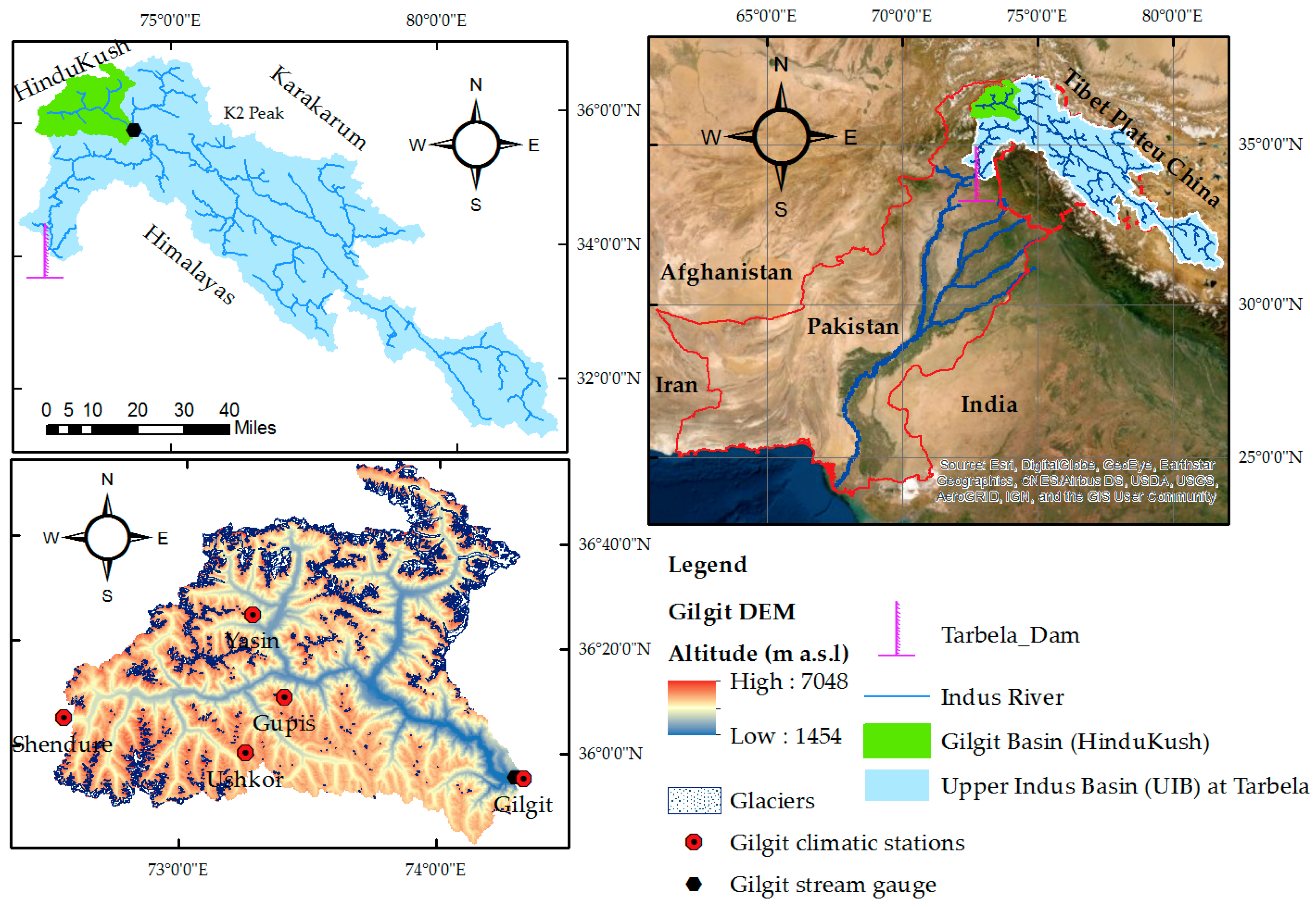
Figure 1. The location map of Gilgit River in the Upper Indus Basin (UIB) of Pakist.
Water 12 01481 g001
Figure 2. Graphical presentations of (a) mean basin temperature (T), discharges at Gilgit gauge (Q), and suspended sediment concentrations (SSC) at Gilgit gauge, (b) mean basin snow covered area (SCA), mean basin rainfall (R), and mean basin evapotranspiration (Evap) for the Gilgit basin during period 1981–2010.
Water 12 01481 g002
Figure 3. Time series plot between the MODIS-observed snow cover fractions and temp-index snow model-simulated snow cover fractions during calibration (2000–2007) and validation periods (2008–2010).
Water 12 01481 g003
Figure 4. Plot of the sediment rating curve (SRC) for the Gilgit gauge.
Water 12 01481 g004
Figure 5. Plot of the best performance measures for predictions of SSY using the ANN, ANFIS-GP, ANFIS-SC, ANFIS-FCM, MARS, and SRC models during the testing phase for the Gilgit basin.
Water 12 01481 g005
Figure 6. Plot of the best performance measures for predictions of SSY using the ANN, ANFIS-GP, ANFIS-SC, ANFIS-FCM, MARS, and SRC models during the testing phase for the Gilgit basin.
Water 12 01481 g006
Figure 7. Overall comparison of the performance measures of coefficient of determination (R2), Nash–Sutcliffe efficiency model performance coefficient (NSE), and root-mean-square error (RMSE) with different input variable scenarios during the testing phase from all models.
Water 12 01481 g007
Figure 8. Plot of the observed vs. predicted SSY using multiple linear regression equation during the training and testing phases for the Gilgit gauging station.
Water 12 01481 g008
Table 1. Data collected for the prediction of suspended sediment yields for the Gilgit River basin.
VariableData SourcePeriodSource
Q *Daily mean discharge (m3/sec)Daily, 1981–2010Water and Power Development Authority (WAPDA), Pakistan
SSC *Suspended sediment concentration (mg/L)Intermittent days per week
1981–2010
Water and Power Development Authority (WAPDA), Pakistan
SCFSnow cover fractions ranging (0–1) extracted from MODIS satellite dataWeekly, basin avg.
2000–2010
https://nsidc.org/data/MOD10A2
TDaily mean, maximum & minimum air temperature (°C) on a 5 × 5 km gridDaily, basin avg.
1981–2010
HI-AWARE project [47,48]
PDaily mean rainfall (mm/day) on a 5 × 5 km gridDaily, basin avg.
1981–2010
HI-AWARE project [47,48]
EvapDaily mean Evapotranspiration (mm/day) on a 5 × 5 km gridDaily, basin avg.
1981–2010
HI-AWARE project [47,48]
Note * The variable of discharge (Q) and suspended sediment concentrations (SSC) are measured at Gilgit gauging station and variables of SCF, T, P, and Evap are basin averages grid datasets.
Table 2. Relationship of Gilgit basin input variables determined by using the Pearson’s correlation coefficient. Log Q: logarithm of water discharges at Gilgit gauge; Log SSY: logarithm of sediment yields at Gilgit gauge; SCA: basin average snow cover area: Tavg: averaged basin mean temperature; P: basin-averaged effective rainfall; Evap: basin averaged evapotranspiration.
log Q
(m3/day)
log SSY
(tons/day)
SCA
(fractions)
Tavg
(°C)
P
(mm)
Evap
(mm/day)
log Q (m3/day)1
log SSY (tons/day)0.871
SCA (fractions)−0.85−0.741
Tavg. (°C)0.870.79−0.881
P (mm)0.160.150.090.11
Evap. (mm/day)0.860.81−0.820.930.061
Table 3. Results of performance measurement statistics during calibration (2000–2007) and validation (2008–2010) periods of the temperature-index snow model for simulations of snow melt and snow cover fractions.
ksnow = 4.2 (mm/day/°C)
Calibration Period (2000–2007)Validation Period (2008–2010)
R20.900.90
NSE0.720.70
RMSE0.150.15
Table 4. Training and testing statistics of the ANN model employing the Levenberg-Marquardt algorithm using different input combinations for the Gilgit basin.
ScenariosModel InputsNeuronsTransfer FunctionR2RMSENSE
InputOutputTrainingTestingTrainingTestingTrainingTesting
S1Qt3logsigpurelin0.760.810.480.420.760.8
S2Qt, Qt−13logsigpurelin0.770.790.480.440.770.79
S3Qt, Qt−1, Qt−25radbaspurlin0.780.790.460.450.780.79
S4Qt, Qt−1, Qt−2, Qt−35tansigpurelin0.800.800.440.470.800.79
S5Qt, Qt−1, Qt−2, Qt−3, Qt−47logsigpurelin0.810.800.430.440.810.80
S6Qt, SCAt5tansigpurelin0.790.820.450.440.790.81
S7Qt, SCAt, SCAt−17tansigtansig0.800.800.440.430.800.8
S8Qt, SCAt, SCAt−1, SCAt−28tansigtansig0.800.810.440.430.800.81
S9Qt, Rt−1, SCAt, SCAt−47logsigpurelin0.800.820.440.420.800.82
S10Qt, Tt−1, Evapt−1, SCAt, SCAt−45radbastansig0.810.820.420.430.810.81
S11Tt3logsigpurelin0.690.730.550.500.690.73
S12Tt, Tt−13logsigtansig0.690.740.540.510.690.73
S13Tt, Tt−1, Tt−26tansigtansig0.740.730.510.510.740.72
S14Tt, Tt−1, Tt−2, Tt−38tansigtansig0.750.740.490.510.750.74
S15Tt, Tt−1, Tt−2, Tt−3, Tt−47radbastansig0.740.760.490.510.740.76
Table 5. Training and testing statistics of the AFIS1 grid partition (GP) model employing different input combinations for the Gilgit basin.
ScenariosModel InputsMembership FunctionsNo of FunctionsR2RMSENSE
TrainingTestingTrainingTestingTrainingTesting
S1Qtpimf40.770.780.460.470.770.78
S2Qt, Qt−1pimf20.780.780.460.470.780.78
S3Qt, Qt−1, Qt−2gauss2mf20.790.770.450.490.790.77
S4Qt, Qt−1, Qt−2, Qt−3gbellmf20.810.750.430.500.810.75
S5Qt, Qt−1, Qt−2, Qt−3, Qt−4trimf20.810.710.430.530.810.69
S6Qt, SCAttrimf20.790.770.450.450.790.77
S7Qt, SCAt, SCAt−1trimf20.790.780.440.470.790.78
S8Qt, SCAt, SCAt−1, SCAt−2trimf20.820.760.420.470.820.75
S9Qt, Rt−1, SCAt, SCAt−4trimf20.820.760.410.490.820.76
S10Qt, Tt−1, Evapt−1, SCAt, SCAt−4trimf20.850.720.380.520.850.72
S11Ttpsigmf20.700.700.550.520.700.70
S12Tt, Tt−1pimf20.710.710.540.510.710.71
S13Tt, Tt−1, Tt−2trimf20.710.730.520.520.710.73
S14Tt, Tt−1, Tt−2, Tt−3trapmf20.720.720.510.530.720.72
S15Tt, Tt−1, Tt−2, Tt−3, Tt−4trimf20.770.600.460.650.770.59
Table 6. Training and testing statistics of the AFIS2 subtractive clustering (SC) model employing different input combinations for the Gilgit basin.
ScenariosModel InputsRadiiR2RMSENSE
TrainingTestingTrainingTestingTrainingTesting
S1Qt0.500.770.780.460.470.770.78
S2Qt, Qt−10.700.770.780.460.470.770.78
S3Qt, Qt−1, Qt−20.700.770.780.460.470.770.78
S4Qt, Qt−1, Qt−2, Qt−30.700.780.780.450.470.780.78
S5Qt, Qt−1, Qt−2, Qt−3, Qt−40.800.780.780.450.470.780.78
S6Qt, SCAt0.600.780.780.450.470.780.78
S7Qt, SCAt, SCAt−10.800.780.780.450.470.780.78
S8Qt, SCAt, SCAt−1, SCAt−20.700.790.770.440.480.790.77
S9Qt, Rt−1, SCAt, SCAt−40.600.790.780.450.470.790.78
S10Qt, Tt−1, Evapt−1, SCAt, SCAt−40.900.800.790.430.460.800.79
S11Tt0.500.700.700.530.550.700.70
S12Tt, Tt−10.600.710.700.520.550.710.70
S13Tt, Tt−1, Tt−20.800.720.720.510.530.720.72
S14Tt, Tt−1, Tt−2, Tt−30.800.720.710.510.540.720.71
S15Tt, Tt−1, Tt−2, Tt−3, Tt−40.700.720.730.510.520.720.73
Table 7. Training and testing statistics of the AFIS3 FCM clustering model employing different input combinations for the Gilgit basin.
ScenariosModel InputsNo of ClustersR2RMSENSE
TrainingTestingTrainingTestingTrainingTesting
S1Qt20.770.780.460.470.770.78
S2Qt, Qt−140.770.780.460.470.770.78
S3Qt, Qt−1, Qt−220.770.780.460.470.780.78
S4Qt, Qt−1, Qt−2, Qt−320.770.780.460.480.770.78
S5Qt, Qt−1, Qt−2, Qt−3, Qt−420.770.780.460.480.770.77
S6Qt, SCAt20.780.780.450.470.780.78
S7Qt, SCAt, SCAt−120.780.780.450.470.780.78
S8Qt, SCAt, SCAt−1, SCAt−220.780.770.450.480.800.78
S9Qt, Rt−1, SCAt, SCAt−420.790.780.440.470.790.78
S10Qt, Tt−1, Evapt−1, SCAt, SCAt−420.800.780.430.470.800.78
S11Tt30.700.700.530.550.700.70
S12Tt, Tt−120.710.700.530.550.710.70
S13Tt, Tt−1, Tt−240.720.710.510.540.720.71
S14Tt, Tt−1, Tt−2, Tt−360.760.720.480.530.760.72
S15Tt, Tt−1, Tt−2, Tt−3, Tt−420.720.700.510.550.720.70
Table 8. Training and testing statistics of the MARS model employing different input combinations for the Gilgit basin.
ScenariosModel InputsBasis
Function
R2RMSENSE
TrainingTestingTrainingTestingTrainingTesting
S1Qt50.770.780.470.470.770.78
S2Qt, Qt−1150.770.780.470.470.770.78
S3Qt, Qt−1, Qt−2150.770.780.470.470.770.78
S4Qt, Qt−1, Qt−2, Qt−3150.770.780.470.470.770.78
S5Qt, Qt−1, Qt−2, Qt−3, Qt−4150.780.780.470.470.770.78
S6Qt, SCAt150.770.780.460.480.780.77
S7Qt, SCAt, SCAt−1200.770.770.460.480.770.77
S8Qt, SCAt, SCAt−1, SCAt−2150.770.770.460.480.770.77
S9Qt, Rt−1, SCAt, SCAt−4250.780.770.450.480.780.77
S10Qt, Tt−1, Evapt−1, SCAt, SCAt−4100.790.790.450.460.790.79
S11Tt200.690.700.540.550.690.70
S12Tt, Tt−1150.700.700.530.550.700.70
S13Tt, Tt−1, Tt−2100.710.710.520.550.710.70
S14Tt, Tt−1, Tt−2, Tt−3100.720.710.520.540.720.71
S15Tt, Tt−1, Tt−2, Tt−3, Tt−4200.720.710.510.540.720.71
Table 9. Comparison of performance measurements by using the SRC, ANFIS-GP, ANFIS-SC, ANFIS-SC, ANFIS-FCM, and MARS models in predictions of sediment yields.
ModelsTraining PeriodTesting Period
R2RMSENSER2RMSENSE
SRC0.810.490.750.710.600.66
ANN0.810.420.810.820.430.81
ANFIS-GP0.790.440.790.780.470.78
ANFIS-SC0.800.430.800.790.460.79
ANFIS-FCM0.800.430.800.780.470.78
MARS0.790.450.790.790.460.79
Table 10. Comparison of the ANFIS-GP, ANFIS-SC, ANFIS-SC, ANFIS-FCM, MARS, and SRC models’ absolute sediment fluxes and relative accuracies (%age) for peak estimations of SSY for the Gilgit gauging station.
YearPeaks > 3200 (tons/day)ANN (tons/day)ANFIS-GP (tons/day)ANFIS-SC (tons/day)ANFIS-FCM (tons/day)MARS (tons/day)SRC (tons/day)
198339013934
(99.15)
3884
(99.56)
3886
(99.62)
3613
(92.62)
3826
(98.07)
4654
(80.69)
198449553542
(71.48)
4543
(91.68)
3033
(61.21)
3789
(76.46)
3385
(68.31)
4375
(88.29)
199132563088
(94.84)
2804
(86.11)
3128
(96.06)
3093
(94.99)
3105
(95.36)
4468
(62.77)
200340572372
(58.46)
2514
(61.96)
2616
(64.48)
2790
(68.77)
2674
(65.91)
4400
(91.54)
200516,89812,993
(76.89)
8949
(52.95)
9480
(56.10)
12,458
(73.72)
12,365
(73.17)
32,385
(8.35)
Mean
(Relative Accuracy %)
66135186
(80.17)
4539
(78.45)
4429
(75.49)
5149
(81.31)
5071
(80.16)
10,056
(66.33)