Pulsating Flow of an Ostwald—De Waele Fluid between Parallel Plates

Abstract

The flow between two parallel plates driven by a pulsatile pressure gradient was studied analytically with a second-order velocity expansion. The resulting velocity distribution was compared with a numerical solution of the momentum equation to validate the analytical solution, with excellent agreement between the two approaches. From the velocity distribution, the analytical computation of the discharge, wall shear stress, discharge, and dispersion enhancements were also computed. The influence on the solution of the dimensionless governing parameters and of the value of the rheological index was discussed.

1. Introduction

The laminar, oscillating flow, driven by a harmonic pressure gradient in Newtonian fluids in pipes has been studied theoretically at least since the work by Sexl in 1930 [1], who obtained the classical velocity profile in the radial direction in terms of the Bessel function of the first kind and order 0. In his paper, Sexl analyzed the behavior of the solution for some limit values of the dimensionless parameter $a\sqrt{\omega /\nu }$, where $a$ is the radius of the tube, $\omega$ the angular frequency of the pressure gradient, and ν the kinematic viscosity of the fluid. In 1952, Lambossy [2] re-analyzed the problem and explicitly concluded that the shape of the velocity profile depended on the dimensionless parameter $\sqrt{\omega /\nu }$. Later, Womersley [3,4] published a paper focusing on flows in arteries, in which it is stressed the importance of the dimensionless parameter used by Sexl and Lambossy, and that became known as Womersley number. The oscillatory flow of non-Newtonian fluids has been studied theoretically by Pipkin [5], Etter and Schowalter [6], and Rahaman and Ramkissoon [7] for viscoelastic fluids, among others. Uchida [8] studied the flow of a Newtonian fluid due to pulsatile pressure gradient (i.e., superposition of oscillatory and constant pressure gradients). Among the analytical studies on pulsatile flows of non-Newtonian fluids, the following works can be mentioned: Barnes et al. [9] for some kind of Oldroyd fluids; Phan-Thien [10,11] and Steller [12] for generalized Maxwell fluids; Davies et al. [13] for the Goddard-Miller model, power-law, and Segalman viscosity functions; Mai and Davis [14] for Bingham plastics; Daprà and Scarpi [15] for power-law fluids. Recognizing the non-Newtonian behavior of the blood [16], an important amount of work has been done addressing the circulation of blood in veins and arteries, stimulating the study of the pulsatile flow of non-Newtonian fluids (for example, references [17,18,19] among others). The most used approach to get the analytical solution of the non-Newtonian pulsatile flow is by means of power expansions, truncated at the first- or second-order, depending on the author. However, the increment of the flow rate with respect to the constant gradient pressure condition can be computed only with a second-order expansion [9,10,11,15]. Because most of the studies have been motivated by the transport of non-Newtonian fluids in the industry or by the blood motion in arteries and veins, the most used configuration corresponds to the flow in a cylinder, or with axial symmetry. Among the few analytical studies in non-cylindrical geometries, the works by Siginer [20] and Steller [12] can be mentioned. The first analyzed the pulsatile plane Pouseille flow of viscoelastic liquids of the memory integral type, and the second the flow of a generalized Maxwell fluid through a slit. Mc Ginty et al. [21] presented solutions of pulsatile flows of Newtonian, Maxwell, and Oldroyd B fluids in a cylinder and in the gap between two cylinders. Daprà and Sacarpi [22] analyzed the later configuration for a Bingham fluid. Letelier et al. [23] solved the pulsating flow of a linearly viscoelastic fluid in straight tubes of arbitrary cross-sections, presenting results of the flow for square and hexagonal ducts with rounded corners. Analytical solutions for two-dimensional configurations are rather scarce when compared with their cylindrical counterpart. In addition to the paper by Steller [12], we can mention those by Daprà and Scarpi [24], who got a perturbation solution to the second-order of the pulsatile flow of a pseudoplastic Williamson fluid, and that by Nandakumar et al. [25] for a shear-thinning fluid in a two-dimensional stenosed channel.

Analytical solutions of pulsatile flows of non-Newtonian fluids are limited to very specific geometries, and they demand long algebraic developments. Thus, numerical approaches have been profusely used. The most used numerical approach to solve the equation of motions is the finite difference method. Among the articles that use this method for solving the pulsating and/or oscillatory flow of non-Newtonian fluids in cylindrical geometry, the following can be mentioned: Edwards et al. (1972, power-law fluid [26]); Balmer and Fiorina (1980, power-law [27]); Adusumilli and Hill (1984, truncated power-law [28]); Nakamura and Sawada (1987, a bi-viscosity model of a Bingham plastic [29]); Warsi (1994, power-law [30]); Mai and Davis (1996, Newtonian, power-law and a modified Bingham plastic [14]); Daprà and Scarpi (2006, power law [15]). Axisymmetric occluded pipes have been studied, for example, by Javadzadegan et al. (2009, Oldroy-B and Cross model [31]). Rectangular or two-dimensional geometries have been studied by Yakhot et al. (1999, Newtonian fluid [32]) and Daprà and Scarpi (2007, Williamson fluid [24]). Flow in the gap of coaxial cylinders of a Bingham fluid under periodic pressure gradient and periodic oscillation of the inner cylinder has been studied by Daprà and Scarpi [22]. The work by Tu and Deville [33] is among the exceptions in which the finite element method is used to solve the pulsatile flow of power-law and Herschel-Bulkley fluids in a cylindrical pipe with an occlusion. Pontrelli [34] complemented an implicit finite difference method in time with a spectral collocation method in space in order to solve the pulsatile flows of fluids modeled as Oldroy-B and an ad hoc blood model.

Most of the experimental studies concerning pulsating flows of non-Newtonian fluids are oriented to determine the enhancement of the temporal mean discharge when compared with the constant pressure gradient driven flow. Some of them also deal with the effect that pressure pulsation has on energy consumption. The motivation of most of the papers comes from studies on blood circulation. Barnes et al. [9] got experimental relationships between the flow enhancement, the frequency of the fluctuation, pressure gradient, and amplitude of the oscillation for Newtonian and shear-thinning fluids generated by an aqueous solution of polyacrylamide. Harris and Maheshwari [35], also with solutions of polyacrylamide, compared the predicted and measured velocity profiles. Their work did not use specific rheological models, but they were within the general class up to second-order viscoelastic fluids.

Thurston [36], in 1975, performed measurements of pressure and volume flow of blood considering steady, oscillatory, and pulsatile flows. The blood is considered a viscoelastic fluid, and the comparison with measurements on a Newtonian glycerol solution helped the authors to specify the special features of the blood flow. Davies and Chakrabarti [37] worked with solutions of polyacrylamide in order to experimentally obtain the enhanced discharge and energy consumption and compared them with the corresponding values for Newtonian fluids. Along the same line, Phan-Thien and Dudek [10] from their experiments with aqueous solutions of Separan AP-30 found that the enhancement decreased with the frequency. Kajiuchi and Saito [38] performed experiments with clay slurries that behaved as Bingham plastics, finding that the flow enhancement could be expressed as a function of the Stokes number for a Bingham plastic fluid, the Bingham number, and the ratio between the pressure oscillation amplitude and the gradient of the base pressure. Lin et al. [39] studied non-colloidal suspensions modeled as Newtonian fluids for a shear rate below a cut value and as power-law fluids for shear rates greater than that value. Among other conclusions, they determined that particle migration might significantly affect flow enhancement.

Most of the researches involving pulsating flows deal with cylindrical or distorted cylindrical geometries because they have been motivated by studies of blood flows in veins and arteries. However, the flow in fractured rocks entails fluid motion through slender gaps that can properly be considered as the flow between parallel plates. The pulsatile flow of shear-thinning fluids through fractured rocks is found in enhanced oil recovery operations [24].

The goal of the present study was to determine analytical solutions for the two-dimensional flow of an Ostwald-de Waele type fluid driven by a pulsating pressure gradient. To accomplish this goal, a perturbation method was used to obtain the velocity distribution up to a second-order term, from which the instantaneous discharge, wall shear stress, cycle-average discharge, and dispersion coefficient were also analytically obtained and computed. A numerical solution using a spectral method was computed in order to check the analytical solution of the velocity distribution. As far as the authors are aware, no solution for the two-dimensional pulsatile flow of an Ostwald—de Waele fluid has been previously published. Daprà and Scarpi [15,24] solved this problem in cylindrical coordinates and used a two-dimensional geometry for a Williamson fluid. The solution presented in this article includes more details of the algebra than reported previously [15,24].

2. Analytical Solution

The laminar, incompressible, two-dimensional, pulsatile flow between two parallel plates of a power-law fluid is governed by the continuity and momentum equations, which are reduced to:

$$\frac{\partial u}{\partial x}=0$$

(1)

$$\rho \frac{\partial u}{\partial t}=-\frac{\partial p}{\partial x}+K\frac{\partial }{\partial y}\left({\left|\frac{\partial u}{\partial y}\right|}^{n-1}\frac{\partial u}{\partial y}\right)$$

(2)

where $p$ is the pressure, $u$ is the velocity component in the $x$ direction, parallel to the plates. The axis $y$ is normal to the plates, with the origin located at the inferior plate. $t$ is the time. $\rho ,K$, and $n$ are the density, consistency coefficient, and flow behaviour index of the fluid, respectively. In pulsatile flow, the pressure gradient is given by:

$$\frac{\partial p}{\partial x}=-P\left(1+\epsilon \sin \omega t\right)$$

(3)

where $\omega$ and $\epsilon$ are the frequency and the relative amplitude of the oscillating part of the pressure gradient, respectively. For infinitely long plates, the velocity is independent of the variable $x$. Two parallel plates separated at a distance $2H$ have a symmetry plane along $y=H$ and non-slip conditions at the plates. Thus, the boundary conditions are

$$u\left(y=0,t\right)=0$$

(4)

$${\frac{\partial u}{\partial y}|}_{\left(y=H,t\right)}=0$$

(5)

Assuming $P>0$ and $\epsilon \ll 1$, the velocity derivative satisfies $\partial u/\partial y\ge 0$ for $0\ge y\ge H$, and Equation (2) becomes:

$$\rho \frac{\partial u}{\partial t}=P\left(1+\epsilon \sin \omega t\right)+K\frac{\partial }{\partial y}\left({\left(\frac{\partial u}{\partial y}\right)}^n\right)$$

(6)

Denoting with an upper asterisk the dimensionless variables:

$$\begin{array}{ccc}\begin{array}{ccc}{u}^{\ast }=\frac{u}{U_0}& ,& y^{\ast }=\frac{y}{H}\end{array}& ,& \begin{array}{ccc}{t}^{\ast }=\omega t& ,& p^{\ast }=\frac{1}{P}\frac{\partial p}{\partial x}=1+\epsilon \sin \left(\omega t\right)\end{array}\end{array}$$

(7)

The velocity scale $U_0$ is not arbitrary and has been defined later. Dropping the asterisks of the dimensionless variables, the momentum equation is written as:

$$\mathsf{\Omega }\frac{\partial u}{\partial t}=\left(1+\epsilon \sin t\right)+\lambda \frac{\partial }{\partial y}\left({\left(\frac{\partial u}{\partial y}\right)}^n\right)$$

(8)

where Ω and λ are dimensionless parameters defined as:

$$\mathsf{\Omega }=\frac{\rho U_0\omega }{P}$$

(9)

$$\lambda =\frac{K{U}_0^n}{P{H}^{n+1}}$$

(10)

As there is not a velocity scale imposed externally to the problem, $U_0$ should depend on the other parameters, i.e., $\rho ,P$, and $H$, resulting $U_0=\sqrt{PH/\rho }$. Thus, the dimensionless frequency becomes

$$\mathsf{\Omega }=\omega \sqrt{\frac{\rho H}{P}}$$

(11)

Replacing $P$ in terms of $U_0$, it is easy to recognize that λ corresponds to the inverse of a Reynolds number associated with power-law fluids, $\lambda =1/Re=\rho U_0^{2-n}{H}^n/K$. In terms of $P$:

$$\lambda =\frac{1}{Re}=\frac{K}{P{H}^{n+1}}{\left(\frac{PH}{\rho }\right)}^{\frac{n}{2}}$$

(12)

Equation (8) becomes:

$$\mathsf{\Omega }\frac{\partial u}{\partial t}=\left(1+\epsilon \sin t\right)+\frac{1}{Re}\frac{\partial }{\partial y}\left({\nu }_{app}\frac{\partial u}{\partial y}\right)$$

(13)

where ${\nu }_{app}$ denotes the apparent viscosity:${\nu }_{app}={\left|\frac{\partial u}{\partial y}\right|}^{n-1}$, with the boundary conditions:

$$u\left(y=0,t\right)=0$$

(14)

$${\frac{\partial u}{\partial y}|}_{\left(y=1,t\right)}=0$$

(15)

The above differential equation will be solved expanding it in a series of $\epsilon$ up to the second-order:

$$u\left(y,t\right)=u_0\left(y\right)+\epsilon u_1\left(y,t\right)+{\epsilon }^2{u}_2\left(y,t\right)+\vartheta \left({\epsilon }^3\right)$$

(16)

Replacing the expansion given by Equation (16) in Equation (13) yields to:

$$\begin{array}{cc}\hfill \epsilon \mathsf{\Omega }\frac{\partial u_1\left(y,t\right)}{\partial t}+{\epsilon }^2& \mathsf{\Omega }\frac{\partial u_2\left(y,t\right)}{\partial t}\hfill \\ & =1+\epsilon \sin \left(t\right)\hfill \\ & +\frac{1}{Re}\frac{\partial }{\partial y}({\left(\frac{\partial u_0}{\partial y}\right)}^n+\left[n{\left(\frac{\partial u_0}{\partial y}\right)}^{n-1}\frac{\partial u_1}{\partial y}\right]\epsilon \hfill \\ & +\left[n{\left(\frac{\partial u_0}{\partial y}\right)}^{n-1}\frac{\partial u_2}{\partial y}+\frac{n\left(n-1\right)}{2!}{\left(\frac{\partial u_0}{\partial y}\right)}^{n-2}{\left(\frac{\partial u_1}{\partial y}\right)}^2\right]{\epsilon }^2)\hfill \end{array}$$

(17)

The solution at the zero-order is the classical result for a power-law fluid, and it is obtained after integrating the following equation

$$0=1+\frac{1}{Re}{\left(\frac{\partial u_0}{\partial y}\right)}^n$$

(18)

with the boundary conditions:

$$u_0\left(y=0\right)=0$$

(19)

$${\frac{\partial u_0}{\partial y}|}_{y=1}=0$$

(20)

resulting the zero order velocity distribution:

$$u_0\left(y\right)=R{e}^{\frac{1}{n}}\left(\frac{n}{n+1}\right)\left[1-{\left(1-y\right)}^{\frac{1}{n}+1}\right]$$

(21)

The unsteady characteristic of the flow is considered from the first-order onwards. Using the solution for $u_0$, the differential equation for order $\epsilon$ is

$$\mathsf{\Omega }\frac{\partial u_1}{\partial t}=\sin \left(t\right)+\frac{1}{Re}\frac{\partial }{\partial y}\left(nR{e}^{\frac{n-1}{n}}{\left({\left(1-y\right)}^{\frac{1}{n}}\right)}^{n-1}\frac{\partial u_1}{\partial y}\right)$$

(22)

Considering that the first-order solution of the velocity has the form:

$$u_1\left(y,t\right)=ℛe\left[W_1\left(y\right)e^{it}\right]$$

(23)

where $ℛe\left[z\right]$ is the real part of the complex $z$, and replacing $u_1$ in Equation (22), the differential equation becomes

$$\mathsf{\Omega }i{W}_1{e}^{it}=-i{e}^{it}+\frac{1}{Re}\frac{\mathrm{d}}{\mathrm{d}y}\left(nR{e}^{\frac{n-1}{n}}{\left(1-y\right)}^{\frac{n-1}{n}}\frac{\mathrm{d}{W}_1}{\mathrm{d}y}\right)e^{it}$$

(24)

Expanding the derivative and rearranging terms, the above equation is written as:

$$\begin{gathered} i=n{\left(\frac{1}{Re}\right)}^{\frac{1}{n}}\left({\left(1-y\right)}^{\frac{n-1}{n}}\frac{{\mathrm{d}}^2{W}_1}{\mathrm{d}{y}^2}-\left(\frac{n-1}{n}\right){\left(1-y\right)}^{-\frac{1}{n}}\frac{\mathrm{d}{W}_1}{\mathrm{d}y}\right){\left(1-y\right)}^{\frac{n-1}{n}}\frac{{\mathrm{d}}^2{W}_1}{\mathrm{d}{y}^2} \\ -{\left(\frac{1}{Re}\right)}^{\frac{1}{n}}\left(n-1\right){\left(1-y\right)}^{-\frac{1}{n}}\frac{\mathrm{d}{W}_1}{\mathrm{d}y}-i\mathsf{\Omega }{W}_1 \end{gathered}$$

(25)

Equation (25) is a non-homogeneous differential equation. The function $W_1$ is split into two components, $W_1=W_{11}+W_{10}$, where $W_{11}$ is the solution of the homogeneous part, and $W_{10}=-1/\mathsf{\Omega }$ the solution of the non-homogeneous one. The differential equation for $W_{11}$ is given by:

$$\eta \frac{{\mathrm{d}}^2{W}_{11}}{\mathrm{d}{\eta }^2}+\frac{n-1}{n}\frac{\mathrm{d}{W}_{11}}{\mathrm{d}\eta }-\frac{i\mathsf{\Omega }}{n}R{e}^{\frac{1}{n}}{\eta }^{\frac{1}{n}}{W}_{11}\left(\eta \right)=0$$

(26)

where the new variable η is defined as:

$$\eta =1-y$$

(27)

Equation (26) is an Emden–Fowler type differential equation, with solution

$$W_{11}\left(\eta \right)=C_1\eta {}^{\frac{1}{2n}}{J}_{(-\nu )}\left(\sigma {\eta }^{\frac{n+1}{2n}}\right)+C_2\eta {}^{\frac{1}{2n}}{J}_{\left(\nu \right)}\left(\sigma {\eta }^{\frac{n+1}{2n}}\right)$$

(28)

where $J_{\left(\nu \right)}$ is the Bessel function of the first kind and order ν. $C_1$ and $C_2$ are the integration constants. $\sigma$ and ν are defined as

$$\begin{array}{ccc}\sigma =\frac{\sqrt{2\mathsf{\Omega }n}R{e}^{\frac{1}{2n}}\left(1-i\right)}{n+1}& ,& \nu =\frac{1}{n+1}\end{array}$$

(29)

Imposing the boundary conditions (Equations (19) and (20)), the values of $C_1$ and $C_2$ are obtained:

$$\begin{array}{ccc}{C}_1=\frac{1}{\mathsf{\Omega }{J}_{-\nu }\left(\sigma \right)}& ,& C_2=0\end{array}$$

(30)

Thus, the first-order term of the velocity is:

$$u_1\left(y,t\right)=ℛe\left[\left({\left(1-y\right)}^{\frac{1}{2n}}\frac{1}{J_{-\nu }\left(\sigma \right)}{J}_{-\nu }\left(\sigma {\left(1-y\right)}^{\frac{n+1}{2n}}\right)-1\right)\frac{e^{it}}{\mathsf{\Omega }}\right]$$

(31)

The second-order involves the solutions of zero and first-order. Using the complex identity ${\left(ℛe\left(z\right)\right)}^2=\frac{1}{2}\left(ℛe\left(z^2\right)+{\left|z\right|}^2\right)$ and ${\left|z{e}^{it}\right|}^2={\left|z\right|}^2$, the differential equation for $u_2\left(y,t\right)$ is written in terms of $\eta$ as

$$\begin{array}{ll}\mathsf{\Omega }\frac{\partial u_2}{\partial t}=-n\frac{1}{Re}& \frac{\partial }{\partial \eta }[-{\left(\frac{1}{Re}\right)}^{\frac{1-n}{n}}{\eta }^{\frac{n-1}{n}}\frac{\partial u_2}{\partial \eta }\\ & +\frac{\left(n-1\right)}{4}{\left(\frac{1}{Re}\right)}^{\frac{2-n}{n}}{\eta }^{\frac{n-2}{n}}\left\{{\left|\frac{\mathrm{d}{W}_1}{\mathrm{d}\eta }\right|}^2+ℛe\left[{\left(\frac{\mathrm{d}{W}_1}{\mathrm{d}\eta }\right)}^2{e}^{2it}\right]\right\}]\end{array}$$

(32)

After some algebra with the Bessel functions, the equation for $u_2$ can be written as

$$\begin{array}{ll}\mathsf{\Omega }\frac{\partial u_2}{\partial t}=-n\frac{1}{Re}& [-{\left(\frac{1}{Re}\right)}^{\frac{1-n}{n}}{\eta }^{\frac{n-1}{n}}\frac{\partial u_2}{\partial \eta }\\ & +\frac{\left(n-1\right)}{4}{\left(\frac{1}{Re}\right)}^{\frac{2-n}{n}}{\eta }^{\frac{n-2}{n}}\{{\left|\left(\frac{n+1}{2n}\right)\left(\frac{\sigma }{\mathsf{\Omega }{J}_{-\nu }\left(\sigma \right)}\right){\eta }^{\frac{2-n}{2n}}{J}_{1-\nu }\left(\sigma {\eta }^{\frac{n+1}{2n}}\right)\right|}^2\\ & +ℛe\left[{\left(\left(\frac{n+1}{2n}\right)\left(\frac{\sigma }{\mathsf{\Omega }{J}_{-\nu }\left(\sigma \right)}\right){\eta }^{\frac{2-n}{2n}}{J}_{1-\nu }\left(\sigma {\eta }^{\frac{n+1}{2n}}\right)\right)}^2{e}^{2it}\right]\left\}\right]\end{array}$$

(33)

The velocity $u_2$ is assumed to be composed by a steady and an unsteady component:

$$u_2\left(\eta ,t\right)=u_{20}\left(\eta \right)+u_{21}\left(\eta ,t\right)$$

(34)

Thus, the steady-state component is obtained from

$$-n\frac{1}{Re}\frac{\partial }{\partial \eta }\left[-{\left(\frac{1}{Re}\right)}^{\frac{1-n}{n}}{\eta }^{\frac{n-1}{n}}\frac{\partial u_{20}}{\partial \eta }+\frac{\left(n-1\right)}{4}{\left(\frac{1}{Re}\right)}^{\frac{2-n}{n}}{\eta }^{\frac{n-2}{n}}{\left|\left(\frac{n+1}{2n}\right)\left(\frac{\sigma }{\mathsf{\Omega }{J}_{-\nu }\left(\sigma \right)}\right){\eta }^{\frac{2-n}{2n}}{J}_{1-\nu }\left(\sigma {\eta }^{\frac{n+1}{2n}}\right)\right|}^2\right]=0$$

(35)

Using ${\left|z\right|}^2=z\overline{z}$, $\overline{J_{\mu }\left(z\right)}=J_{\mu }\left(\overline{z}\right)$, the expression for the series expansion of the product of Bessel functions (reference [40], page 148), the term ${\left|J_{1-\nu }\left(\sigma {\eta }^{\frac{n+1}{2n}}\right)\right|}^2$, can be written as

$$J_{1-\nu }\left(\sigma {\eta }^{\frac{n+1}{2n}}\right)J_{1-\nu }\left(\overline{\sigma }{\eta }^{\frac{n+1}{2n}}\right)={\displaystyle \sum }_{m=0}^{\infty }{C}_m{\eta }^{\frac{\left(n+1\right)}{n}m+1}$$

(36)

with

$$C_m=\sqrt{\pi }{\left(\frac{{\left|\sigma \right|}^2}{4}\right)}^{\frac{n}{n+1}}\frac{{\left(-1\right)}^m{\left(\frac{\sigma }{2}\right)}^{2m}}{2^{-m}m!\mathsf{\Gamma }\left(m+2-\nu \right)\mathsf{\Gamma }\left(\frac{1}{2}-\frac{m}{2}\right)\mathsf{\Gamma }\left(\frac{m}{2}-\nu +2\right)}$$

(37)

Thus, the differential equation for $u_{20}$ is given by

$$0=\frac{\partial }{\partial \eta }\left[{\eta }^{\frac{n-1}{n}}\frac{\partial u_{20}}{\partial \eta }-b{\displaystyle \sum }_{m=0}^{\infty }{C}_m{\eta }^{\frac{\left(n+1\right)}{n}m+1}\right]$$

(38)

where

$$b=\frac{\left(n-1\right)}{4}{\left(\frac{1}{Re}\right)}^{\frac{1}{n}}{\left(\frac{n+1}{2n}\right)}^2{\left|\frac{\sigma }{\mathsf{\Omega }{J}_{-\nu }\left(\sigma \right)}\right|}^2$$

(39)

Given the structure of Equation (38), a series solution for $u_{20}$ is feasible, resulting:

$$u_{20}\left(y\right)={\displaystyle \sum }_{m=0}^{\infty }{a}_m\left(1-{\left(1-y\right)}^{\frac{\left(n+1\right)\left(2m+1\right)}{n}}\right)$$

(40)

where the coefficients $a_m$ are given by:

$$a_m=\frac{n\left(1-n\right)}{4\left(1+n\right)}\frac{\sqrt{\pi }{\left(\frac{{\left|\sigma \right|}^2}{4}\right)}^{\frac{n}{n+1}}{\left(\frac{1}{Re}\right)}^{\frac{1}{n}}{\left(\frac{n+1}{2n}\right)}^2{\left|\frac{\sigma }{\mathsf{\Omega }{J}_{-\nu }\left(\sigma \right)}\right|}^2{\left(\frac{\sqrt{\mathsf{\Omega }n}R{e}^{\frac{1}{2n}}}{1+n}\right)}^{4m}{\left(-1\right)}^m}{\left(2m\right)!\left(2m+1\right)\mathsf{\Gamma }\left(2m+2-\nu \right)\left(\frac{1}{2}-m\right)\mathsf{\Gamma }\left(m+2-\nu \right)}$$

(41)

Obviously, the solution given by Equation (40) satisfies the boundary conditions.

The differential equation for the unsteady part of the second-order solution is:

$$\begin{array}{l}\mathsf{\Omega }\frac{\partial u_{21}}{\partial t}\\ =-n\frac{1}{Re}\frac{\partial }{\partial \eta }[-{\left(\frac{1}{Re}\right)}^{\frac{1-n}{n}}{\eta }^{\frac{n-1}{n}}\frac{\partial u_{21}}{\partial \eta }\\ +\frac{\left(n-1\right)}{4}{\left(\frac{1}{Re}\right)}^{\frac{2-n}{n}}{\eta }^{\frac{n-2}{n}}ℛe\left[{\left(\left(\frac{n+1}{2n}\right)\left(\frac{\sigma }{\mathsf{\Omega }{J}_{-\nu }\left(\sigma \right)}\right){\eta }^{\frac{2-n}{2n}}{J}_{1-\nu }\left(\sigma {\eta }^{\frac{n+1}{2n}}\right)\right)}^2{e}^{2it}\right]]\end{array}$$

(42)

The structure of $u_{21}$ is similar to that for the unsteady part of the first-order solution, i.e.,

$$u_{21}\left(\eta ,t\right)=ℛe\left[W_{21}\left(\eta \right)e^{2it}\right]$$

(43)

$W_{21}$ is obtained from:

$$\frac{\partial }{\partial \eta }\left[{\eta }^{\frac{n-1}{n}}\frac{\partial W_{21}}{\partial \eta }\right]+\left(-\frac{2i\mathsf{\Omega }}{n}R{e}^{\frac{1}{n}}\right)W_{21}=\frac{\partial }{\partial \eta }\left[b{J}_{\nu -1}^2\left(\sigma {\eta }^{\frac{n+1}{2n}}\right)\right]$$

(44)

After a rather cumbersome algebra:

$$W_{21}\left(\eta \right)={\displaystyle \sum }_{m=0}^{\infty }{\beta }_m\left\{{\eta }^{\left(\frac{n+1}{n}\right)\left(m+1\right)}-\frac{\eta {}^{\frac{1}{2n}}{J}_{-\nu }\left(\sqrt{2}\sigma {\eta }^{\frac{n+1}{2n}}\right)}{J_{-\nu }\left(\sqrt{2}\sigma \right)}\right\}$$

(45)

with ${\beta }_m$ given by the recurrence equation:

$${\beta }_{m+1}=\frac{b{S}_{m+1}}{\left[\left(\frac{n+1}{n}\right)\left(m+2\right)\right]}+\frac{2i}{{\left(\frac{1}{Re}\right)}^{\frac{1}{n}}n\left[\left(\frac{n+1}{n}\right)\left(m+2\right)\right]\left[\left(\frac{n+1}{n}\right)\left(m+1\right)+1\right]}{\beta }_m$$

(46)

where

$${\beta }_0={\left(\frac{1}{Re}\right)}^{\frac{1}{n}}\frac{n\left(n-1\right)}{4}{\left[\frac{\sigma }{J_{-\nu }\left(\sigma \right)\mathsf{\Omega }}\left(\frac{n+1}{2n}\right)\right]}^2\frac{1}{\left(1+n\right){\mathsf{\Gamma }}^2\left(2-\nu \right)}{\left(\frac{\sigma }{2}\right)}^{2-2\nu }$$

(47)

and

$$S_{m+1}=\frac{{\left(-1\right)}^m\mathsf{\Gamma }\left(5-2\nu +2m\right)}{m!\mathsf{\Gamma }\left(4-2\nu +m\right){\mathsf{\Gamma }}^2\left(2-\nu +m+1\right)}{\left(\frac{\sigma }{2}\right)}^{2m+4-2\nu }$$

(48)

Finally, the second-order term of the velocity is:

$$\begin{array}{ll}{u}_2\left(y,t\right)={\displaystyle {\displaystyle \sum }_{m=0}^{\infty }}{a}_m& \left(1-{\left(1-y\right)}^{\frac{\left(n+1\right)\left(2m+1\right)}{n}}\right)\\ & +ℛe\left\{e^{2it}{\displaystyle {\displaystyle \sum }_{m=0}^{\infty }}{\beta }_m\right[{\left(1-y\right)}^{\left(\frac{n+1}{n}\right)\left(m+1\right)}\\ & -\frac{{\left(1-y\right)}^{\frac{1}{2n}}{J}_{-\nu }\left(\sigma \sqrt{2}{\left(1-y\right)}^{\frac{n+1}{2n}}\right)}{J_{-\nu }\left(\sigma \sqrt{2}\right)}]\}\end{array}$$

(49)

Thus, inserting the solutions given by Equations (21), (31), and (49) into Equation (16), the velocity distribution up to the second-order is obtained. The shear stress is made dimensionless with $\rho U_0^2$, and it is computed directly from

$${\tau }_{xy}=\frac{1}{Re}{\left(\frac{\partial u}{\partial y}\right)}^n$$

(50)

After some algebra, the second-order approximation of ${\tau }_{xy}$ is found to be:

$$\begin{array}{ll}{\tau }_{xy}=\frac{1}{Re}(R{e}^{\frac{1}{n}}& {\left(1-y\right)}^{\frac{1}{n}}+\epsilon ℛe\left[\left(\frac{n+1}{2n}\right)\left(\frac{\sigma }{\mathsf{\Omega }{J}_{-\nu }\left(\sigma \right)}\right){\left(1-y\right)}^{\frac{2-n}{2n}}{J}_{1-\nu }\left(\sigma {\left(1-y\right)}^{\frac{n+1}{2n}}\right)e^{it}\right]\\ & +{\epsilon }^2[{\displaystyle {\displaystyle \sum }_{m=0}^{\infty }}{a}_m\left(\frac{\left(n+1\right)\left(2m+1\right)}{n}{\left(1-y\right)}^{\frac{2mn+2m+1}{n}}\right)\\ & +ℛe\left\{e^{2it}{\displaystyle {\displaystyle \sum }_{m=0}^{\infty }}{\beta }_m\right[-\left(\frac{n+1}{n}\right)\left(m+1\right){\left(1-y\right)}^{\frac{mn+m+1}{n}}\\ & +\left(\frac{n+1}{2n}\right)\left(\frac{\sigma \sqrt{2}}{J_{-\nu }\left(\sigma \sqrt{2}\right)}\right)\left(1-y\right){}^{\frac{2-n}{2n}}{J}_{1-\nu }\left(\sigma \sqrt{2}{\left(1-y\right)}^{\frac{n+1}{2n}}\right)\left]\right\}]{)}^n\end{array}$$

(51)

from where the shear stress acting on the bottom ($y=0$) is determined:

$$\begin{array}{ll}{\tau }_o\left(t\right)=\frac{1}{Re}({\left(Re\right)}^{\frac{1}{n}}& +\epsilon ℛe\left[\left(\frac{n+1}{2n}\right)\left(\frac{\sigma }{\mathsf{\Omega }{J}_{-\nu }\left(\sigma \right)}\right)J_{1-\nu }\left(\sigma \right)e^{it}\right]\\ & +{\epsilon }^2[{\displaystyle {\displaystyle \sum }_{m=0}^{\infty }}{a}_m\frac{\left(n+1\right)\left(2m+1\right)}{n}\\ & +ℛe\left\{e^{2it}{\displaystyle {\displaystyle \sum }_{m=0}^{\infty }}{\beta }_m\right[\left(\frac{n+1}{2n}\right)\left(\frac{\sigma \sqrt{2}}{J_{-\nu }\left(\sigma \sqrt{2}\right)}\right)J_{1-\nu }\left(\sigma \sqrt{2}\right)\\ & -\frac{\left(n+1\right)\left(m+1\right)}{n}\left]\right\}]{)}^n\end{array}$$

(52)

It is easy to show that the bottom shear stress averaged on a cycle is equal to the value associated with the steady flow, i.e., $⟨{\tau }_o⟩=1$, where the angular bracket denotes cycle average.

2.1. Flow Enhancement

The instantaneous dimensionless discharge can be expressed as

$$q\left(t\right)=q_0+\epsilon q_1\left(t\right)+{\epsilon }^2{q}_2\left(t\right)$$

(53)

where

$$q_0={{\displaystyle \int }}_0^1{u}_0\left(y\right)\mathrm{d}y=\frac{n}{2n+1}R{e}^{\frac{1}{n}}$$

(54)

$$q_1\left(t\right)=\epsilon {{\displaystyle \int }}_0^1ℛe\left[\left({\left(1-y\right)}^{\frac{1}{2n}}\frac{1}{J_{-\nu }\left(\sigma \right)}{J}_{-\nu }\left(\sigma {\left(1-y\right)}^{\frac{n+1}{2n}}\right)-1\right)\frac{e^{it}}{\mathsf{\Omega }}\right]\mathrm{d}y$$

(55)

$$\begin{array}{ll}{q}_2\left(t\right)={\epsilon }^2{\displaystyle {{\displaystyle \int }}_0^1}& [{\displaystyle {\displaystyle \sum }_{m=0}^{\infty }}{a}_m\left(1-{\left(1-y\right)}^{\frac{\left(n+1\right)}{n}\left(2m+1\right)}\right)\\ & +ℛe\left\{e^{2it}{\displaystyle {\displaystyle \sum }_{m=0}^{\infty }}{\beta }_m\right[{\left(1-y\right)}^{\left(\frac{n+1}{n}\right)\left(m+1\right)}\\ & -\frac{\left(1-y\right){}^{\frac{1}{2n}}{J}_{-\nu }\left(\sigma \sqrt{2}{\left(1-y\right)}^{\frac{n+1}{2n}}\right)}{J_{-\nu }\left(\sigma \sqrt{2}\right)}\left]\right\}]\mathrm{d}y\end{array}$$

(56)

The flow enhancement is defined as $I_q=\left(⟨q⟩-q_S\right)/q_S$, where $⟨q⟩$ is the average discharge of the pulsatile flow along a period of fluctuation, and $q_S$ is the discharge associated with the steady component of the pressure gradient. In this problem, $q_S=q_0$. Contribution of $q_1$ is nil, resulting in that the flow enhancement is only due to $q_2$. The second-order discharge (Equation (56)) has two addends, but as the second one depends on $e^{2it}$, it does not contribute to the increment of discharge in a period. Thus, the flow enhancement is given by:

$$I_q={\epsilon }^2\frac{1}{R{e}^{\frac{1}{n}}}\frac{2n+1}{n}{\displaystyle \sum }_{m=0}^{\infty }{a}_m\frac{\left(2m+1\right)\left(n+1\right)}{\left(2m+1\right)\left(n+1\right)+n}$$

(57)

In the above equation, $a_m$ is obtained from Equation (41).

The analytical expression for the flow enhancement when inertia is negligible can be obtained, making zero the left-hand-side of Equation (8) and integrating along $y$, resulting $I_q={\epsilon }^2\frac{1-n}{4n^2}$. This is the same discharge increment than for a pulsating flow in a cylindrical pipe [37]. The dimensionless cycle-averaged cross-section-mean-velocity is easily computed from Equation (53), resulting $⟨U⟩=\left(2n/\left(2n+1\right)\right)R{e}^{\frac{1}{n}}\left(1+{\epsilon }^2\left(1-n\right)/\left(4n^2\right)\right)$.

2.2. Dispersion Coefficient

The dimensionless coefficient of longitudinal dispersion, ${\mathcal{K}}^{\ast }$, is defined as ([41], p.86)

$${\mathcal{K}}^{\ast }=\frac{\mathcal{K}D}{U_o^2{h}^2}=-{{\displaystyle \int }}_0^1{u}^{\prime }\left(y\right)\left[{{\displaystyle \int }}_0^y\left({{\displaystyle \int }}_0^{\tilde{y}}{u}^{\prime }\left(\widehat{y}\right)\mathrm{d}\widehat{y}\right)\mathrm{d}\tilde{y}\right]\mathrm{d}y$$

(58)

where $\mathcal{K}$ is the dispersion coefficient, $D$ is the coefficient of molecular diffusion, and $u^{\prime }$ is the dimensionless velocity deviation from the vertical average $\left(\overline{u}\right)$. The structure of the triple integral given by Equation (58) precludes us to look for a second-order analytical solution for ${\mathcal{K}}^{\ast }$, but it is possible to compute its cycle-average value. The dimensionless dispersion coefficient averaged in a period of oscillation is $⟨{\mathcal{K}}^{\ast }⟩=\frac{1}{2\pi }{{\displaystyle \int }}_0^{2\pi }{\mathcal{K}}^{\ast }\mathrm{d}t$. The order of integration can be changed using the Fubini theorem [42], and the cycle average is computed from $⟨{\mathcal{K}}^{\ast }⟩=-{{\displaystyle \int }}_0^1\left[{{\displaystyle \int }}_0^y\left({{\displaystyle \int }}_0^{\tilde{y}}\left\{\frac{1}{2\pi }{{\displaystyle \int }}_0^{2\pi }{u}^{\prime }\left(y\right)u^{\prime }\left(\widehat{y}\right)\mathrm{d}t\right\}\mathrm{d}\widehat{y}\right)\mathrm{d}\tilde{y}\right]\mathrm{d}y$. The velocity deviation contains terms involving $e^{it}$ and $e^{i2t}$, whose integrals in a period are nil. Thus, it is not necessary to carry out the triple integrals in $y$ for many of the terms that appear in Equation (58). Then, the inner integral is:

$$\begin{array}{ll}\frac{1}{2\pi }{{\displaystyle \int }}_0^{2\pi }{u}^{\prime }\left(y\right)u^{\prime }\left(\widehat{y}\right)\mathrm{d}t& \\ & =\left(u_0\left(y\right)-{\overline{u}}_0\right)\left(u_0\left(\widehat{y}\right)-{\overline{u}}_0\right)\\ & +{\epsilon }^2\left[\left(u_0\left(y\right)-{\overline{u}}_0\right)\left(u_{20}\left(\widehat{y}\right)-{\overline{u}}_{20}\right)+\left(u_0\left(\widehat{y}\right)-{\overline{u}}_0\right)\left(u_{20}\left(y\right)-{\overline{u}}_{20}\right)\right]\end{array}$$

(59)

From the above result, it is easy to see that the cycle averaged dispersion coefficient has the structure

$$⟨{\mathcal{K}}^{\ast }⟩=⟨{\mathcal{K}}^{\ast }⟩{}_0+{\epsilon }^2⟨{\mathcal{K}}^{\ast }⟩{}_{20}$$

(60)

with

$$⟨{\mathcal{K}}^{\ast }⟩{}_0=\frac{2n^4}{3{\left(2n+1\right)}^2\left(4n+1\right)\left(5n+2\right)}R{e}^{\frac{2}{n}}$$

(61)

and

$$\begin{array}{ll}⟨{\mathcal{K}}^{\ast }⟩{}_{20}=-{{\displaystyle \int }}_0^1& \left[{\displaystyle {{\displaystyle \int }}_0^y}\right({\displaystyle {{\displaystyle \int }}_0^{\tilde{y}}}[\left(u_0\left(y\right)-{\overline{u}}_0\right)\left(u_{20}\left(\widehat{y}\right)-{\overline{u}}_{20}\right)\\ & +\left(u_0\left(\widehat{y}\right)-{\overline{u}}_0\right)\left(u_{20}\left(y\right)-{\overline{u}}_{20}\right)\left]\mathrm{d}\widehat{y}\right)\mathrm{d}\tilde{y}]\mathrm{d}y\end{array}$$

(62)

After some rather boring algebra, the term accompanying ${\epsilon }^2$ can be computed, and the cycle averaged dispersion coefficient is found to be:

$$⟨{\mathcal{K}}^{\ast }⟩=\frac{2n^4}{3{\left(2n+1\right)}^2\left(4n+1\right)\left(5n+2\right)}R{e}^{\frac{2}{n}}+{\epsilon }^{2}R{e}^{\frac{1}{n}}\frac{2n^3\left(n+1\right)}{3\left(2n+1\right)\left(4n+1\right)}{\displaystyle \sum }_{m=0}^{\infty }{A}_{m,n}$$

(63)

where

$$A_{m,n}=a_m\left[\frac{\left(2m+1\right)\left(2mn+2m+8n+2\right)}{\left(2mn+2m+2n+1\right)\left(2mn+2m+4n+1\right)\left(2mn+2m+5n+2\right)}\right]$$

(64)

The dispersion enhancement is given by $I_{{\mathcal{K}}^{\ast }}=(⟨{\mathcal{K}}^{\ast }⟩-⟨{\mathcal{K}}^{\ast }{⟩}_0)/⟨{\mathcal{K}}^{\ast }⟩{}_0$. Because the intricacy of the coefficient of second-order, it is not possible to get a simpler expression like that obtained for the discharge (Equation (57)).

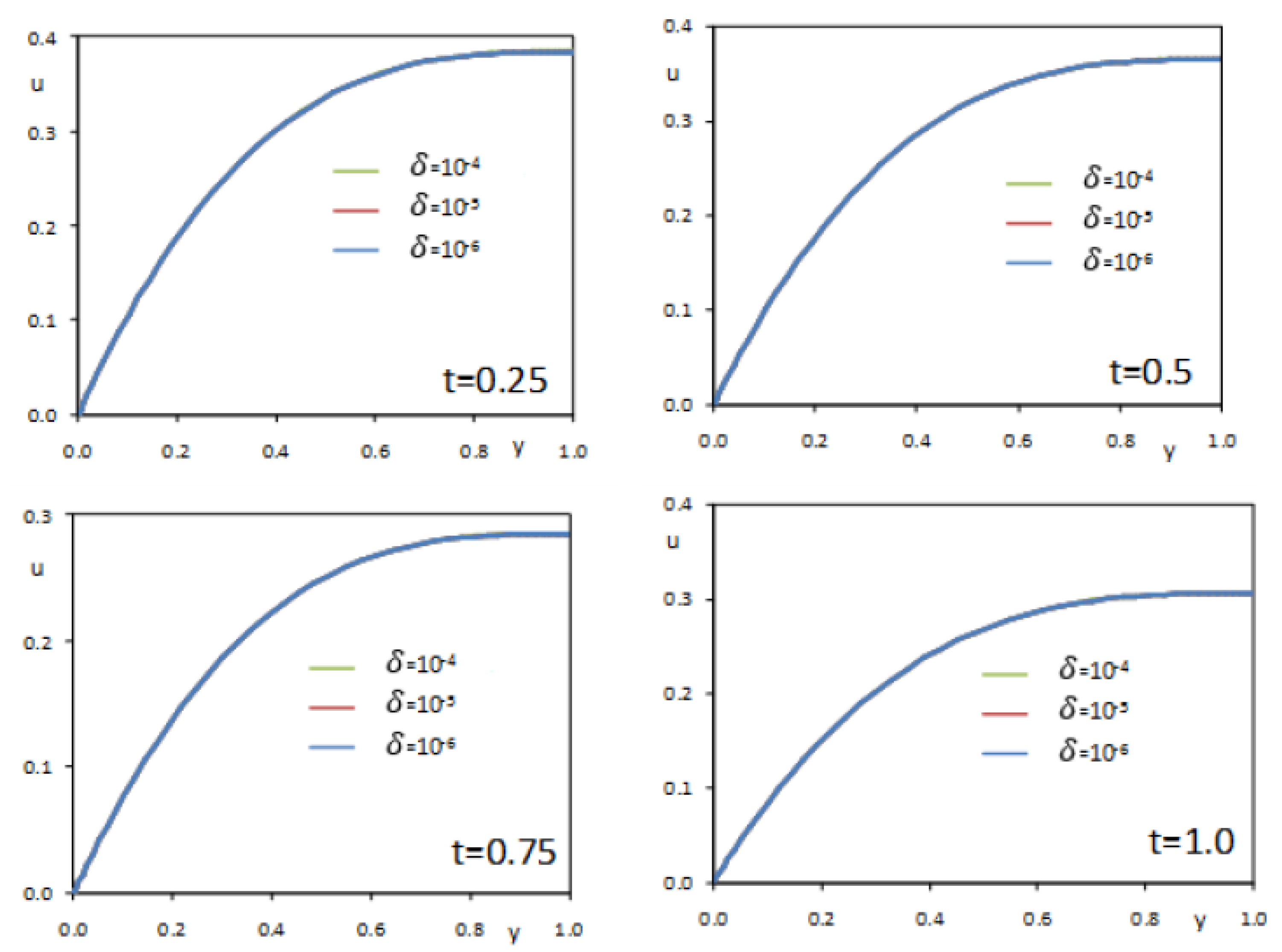
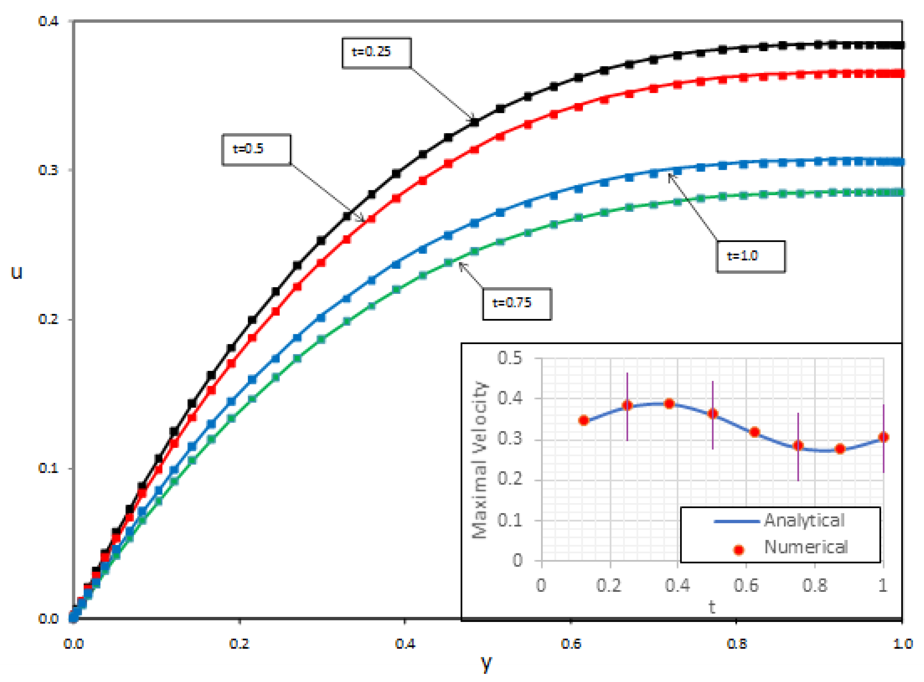
3. Numerical Solution of the Velocity Distribution

In order to verify the correctness of the analytical expression of the velocity profiles reported in the previous section, Equation (13) has been numerically integrated with a spectral method. Spectral methods constitute the most confident approach to the solution of fluid mechanics equations for both Newtonian (see for instance [43,44,45]) and non-Newtonian (see for instance [46,47,48]) fluids, reducing at the minimum the impact of the numerical scheme on the physics of the flow under investigation. Moreover, the higher computational cost of these methods is widely compensated by their fast (exponential) rate of convergence [49]. The spatial discretization of Equation (13), along with the boundary conditions (14)–(15), has been carried out through a spectral patching collocation method based on Gauss–Lobatto–Chebyshev quadrature nodes (see for instance [50]). Denoted with $y_i$, with $i=1,\dots N$, the $N+1$ nodes are obtained by the image of the $N+1$ Gauss–Lobatto–Chebyshev points $x_i=\cos \left(\pi i/N\right)$ by an affine transformation mapping of [1;−1] onto [0,1], and being $u_j=u\left(y_j\right)$, the semi-discretized version of Equation (13) reads

$$\mathsf{\Omega }\frac{\partial u_i}{\partial t}=\left(1+\epsilon \sin \omega t\right)+\frac{1}{Re}{\displaystyle \sum }_{j=1}^{N+1}{D}_{ij}{\eta }_j{\displaystyle \sum }_{h=1}^{N+1}{D}_{jh}{u}_h\hspace{1em}\hspace{1em}\forall i=1,\dots N-1$$

(65)

where $D_{ij}$ is the $ij$-term of the Chebyshev collocation derivative matrix [49], and ${\eta }_j$ the value of the apparent viscosity pertaining to the $y_j$ grid point. In order to deal with the unbounded shear stress gradients associated with the non-Newtonian power-law model, we have adjusted the power-law model by replacing the apparent viscosity ${\nu }_{app}$ as follows [51,52,53]:

$${\nu }_{app}={\left[\delta +{\left(\frac{\partial u}{\partial y}\right)}^2\right]}^{\frac{n-1}{2}}$$

(66)

with $\delta$ an adjustment parameter for which non-negative values have to be prescribed. When $\delta =0$, the standard power-law model is recovered. The influence of the $\delta$ value on the results has been discussed later on. The homogeneous Dirichlet and Neumann boundary conditions (14) and (15) are enforced as follows:

$$u_0=0$$

(67)

$${\displaystyle \sum }_{h=1}^{N+1}{D}_{N+1h}{u}_h=0$$

(68)

The time discretization of Equation (58) has been carried out with a second-order Crank–Nicolson implicit method, iteratively solving the algebraic non-linear system at each time step.

With reference to the $n=0.5$, case Figure 1 puts in evidence the effect of the $\delta$ value on the numerically computed velocity profile for the case $Re=1$, $\mathsf{\Omega }=1$, and $\epsilon =0.1$. Four instants are shown, namely, $t=0.25,0.5,0.75,1.0,$ and three different values of the adjustment parameter $\delta$ have been considered, namely, 10⁻⁴, 10⁻⁵, 10⁻⁶.

Figure 1. Effects of the adjustment parameter $\delta$ on the velocity profiles. $n=0.5,Re=1,\mathsf{\Omega }=1$, and $\epsilon =0.1$.

Figure 1 shows that the results are essentially independent of the $\delta$ value. Similar results (not shown herein) have been obtained, varying each parameter of the $\left(Re,\mathsf{\Omega }\right)$ pair in the range (1, 100). In what follows the value $\delta ={10}^{-5}$ has been considered.

Figure 2 compares the velocity profiles analytically deduced with the corresponding ones numerically calculated. Four instants have been considered, namely, $t=0.25,0.5,0.75,1.0$. The power-law exponent $n$ is equal to 0.5, while the Reynolds number, the pulsation $\mathsf{\Omega }$, and the $\epsilon$ coefficient are 1.0, 1.0, and 0.1, respectively. Figure 2 shows that the analytical solution is in very good agreement with the numerical one, for all instants.

Figure 2. Comparison between analytical (lines) and numerical (symbols) velocity profiles. $n=0.5,Re=1,$ $\mathsf{\Omega }=1$, and $\epsilon =0.1$. The inset shows the pulsation of the maximum velocity (reached at $y=1$). The vertical lines in the inset are indicative of the times at which the velocity profiles were plotted in the main figure.

With the aim of investigating the range of applicability of the deduced analytical solution, in Table 1 and Table 2 the maximum percentual difference between the analytical and numerical solutions, in terms of discharge and wall shear stress, is shown. Four instants in the oscillating period, i.e., $t=0.25,0.50,0.75,1.0$, have been considered. The values of the power-law exponent and of the oscillation amplitude have been fixed equal to 0.5 and 0.1, respectively. Both the frequency and Reynolds number have been varied of two orders of magnitude.

Table 1. Discharge percentage error ($n=0.5$, $\epsilon =0.1$).

	$\mathit{t}=0.25$	$\mathit{t}=0.50$	$\mathit{t}=0.75$	$\mathit{t}=1.00$
$Re=1,\mathsf{\Omega }=1$	−1.6%	−1.8%	−2.0%	−1.9
$Re=100,\mathsf{\Omega }=1$	−0.4%	−0.4%	−0.4%	−0.4%
$Re=1,\mathsf{\Omega }=100$	−0.7%	−0.7%	−0.7%	−0.7%

Table 2. Wall shear stress percentage error ($n=0.5$, $\epsilon =0.1$).

	$\mathit{t}=0.25$	$\mathit{t}=0.50$	$\mathit{t}=0.75$	$\mathit{t}=1.00$
$Re=1,\mathsf{\Omega }=1$	0.4%	−0.1%	0.6%	−0.1%
$Re=100,\mathsf{\Omega }=1$	0.6%	0.6%	−0.3%	−0.3%
$Re=1,\mathsf{\Omega }=100$	Less than 0.1%	Less than 0.1%	Less than 0.1%	Less than 0.1%

Smaller values of ε lead to a reduction of both percentage errors (results not shown). It follows that, for sufficiently small values of $\epsilon$, i.e., smaller than 0.1, the analytical solution may be confidently applied in a large range of Reynolds number and frequency values.

As expected, similar conclusions cannot be drawn when the oscillation amplitude is increased. Indeed, Table 3, where both the percentual errors in the case $\epsilon =0.5$, $Re=1,$ Ω$=1$, and $n=0.5$ are reported, shows that as the perturbation parameter is increased, the accuracy of the proposed solution, as it could be expected, significantly reduces.

Table 3. Percentage errors ($n=0.5$, $\epsilon =0.5$, $Re=1.0$, Ω $=1$).

	$\mathit{t}=0.25$	$\mathit{t}=0.50$	$\mathit{t}=0.75$	$\mathit{t}=1.00$
Discharge	−14.9%	−19.7%	−84.9%	−42.8%
Wall shear stress	6.7%	−1.9%	30.9%	−3.5%

4. Results

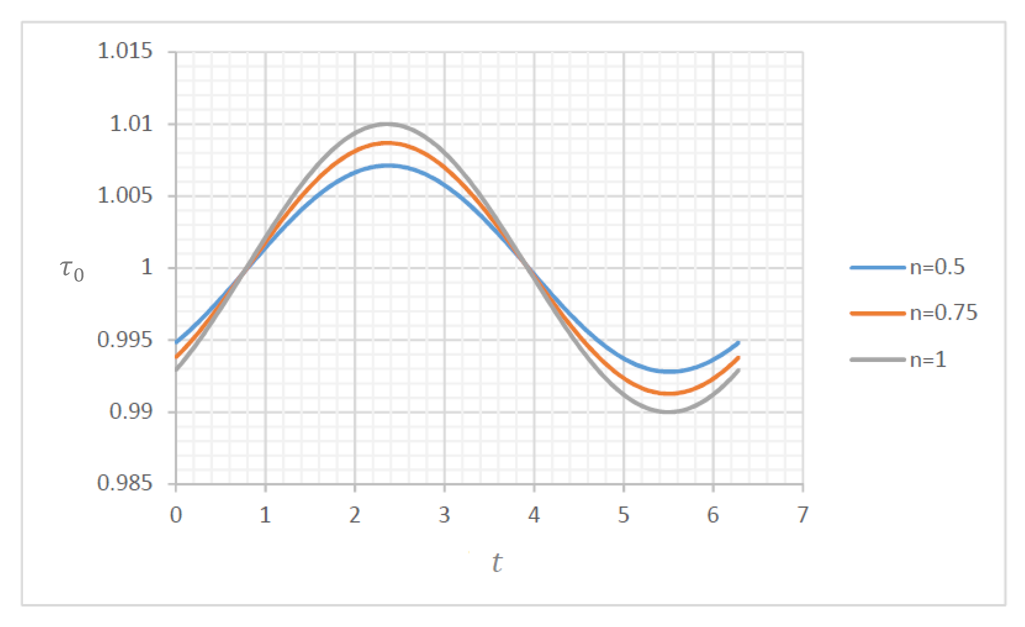
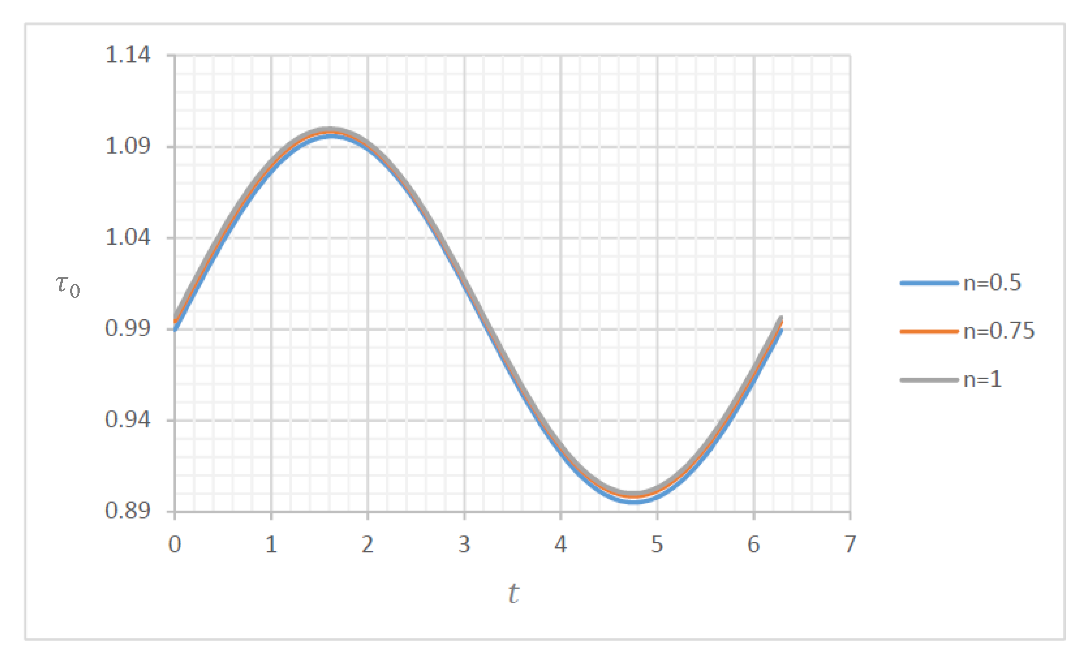
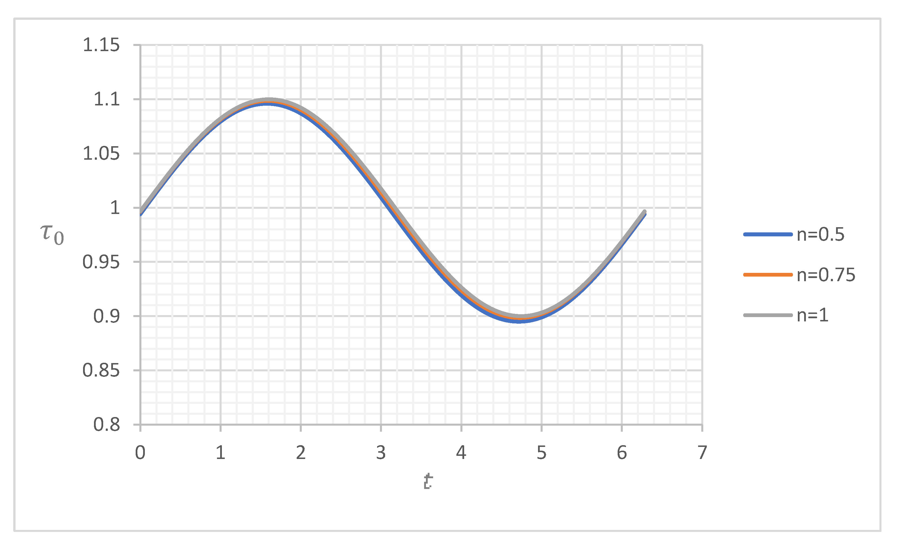
4.1. Wall Shear Stress

The wall shear stress is given by Equation (52). Due to the cumbersome structure of the relationship, it was not feasible to determine analytically some characteristics like the mean, maximum, and minimum values of the wall shear stress. Some limit behaviours of ${\tau }_0$ were analyzed for values of the flow index $n=$ 0.5, 0.75, and 1 (shown below).

4.1.1. Wall Shear Stress for $\mathsf{\Omega }\gg 1$ and $Re~1$

For large dimensionless frequency and $Re~1$, Equation (13) indicates that $\mathsf{\Omega }\partial u/\partial t~\partial \tau /\partial y$, i.e., the contribution of the fluctuating part was negligible, as it is corroborated in Figure 3, where the values $\mathsf{\Omega }=100,Re=1$, and $\epsilon =0,1$ were used. It was observed that the amplitude deviated at the most 1% from the non-pulsating condition (for $n=1$). Also, it showed a delay of the response with respect to the pressure fluctuation. The non-linearity reduced even more the pulsation, already reduced by the effect of large Ω, with a decrease in amplitude as the flow index decreased.

Figure 3. Wall shear stress for $\mathsf{\Omega }=100$, $Re=1$, $\epsilon =0.1$.

4.1.2. Wall Shear Stress for $\mathsf{\Omega }\ll 1$ and $Re~1$

For small Ω and $Re~1$, the terms of first- and second-order in the solution of ${\tau }_0$ became important as they were divided by Ω, resulting in higher amplitude fluctuations, as it is observed in Figure 4, computed for $\mathsf{\Omega }=0,1,Re=1$, and $\epsilon =0.1$.

Figure 4. Wall shear stress for $\mathsf{\Omega }=0.1$, $Re=1$, $\epsilon =0.1$.

4.1.3. Wall Shear Stress for $Re\gg 1$ and $\mathsf{\Omega }~1$

For large $Re$, the effect of Ω was negligible, and ${\tau }_0\to 1+\left(n/R{e}^{1/n}\right)O\left(\epsilon \right)\approx 1$, independently of the flow index, as it is shown in Figure 5, with $\mathsf{\Omega }=1,Re=100$, and $\epsilon =0.1$. The maximum difference from ${\tau }_0=1$ was obtained for a Newtonian fluid and was about 1%. When $n=0.5$, this difference was reduced to 0.1%.

Figure 5. Wall shear stress for $\mathsf{\Omega }=1$, $Re=100$, $\epsilon =0.1$.

4.1.4. Wall Shear Stress for $Re\ll 1$ and $\mathsf{\Omega }~1$

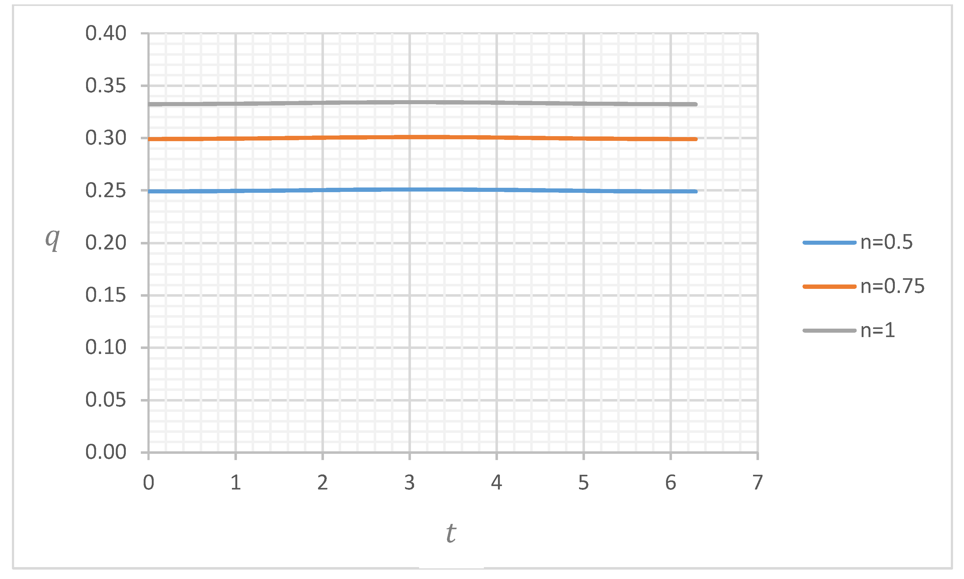
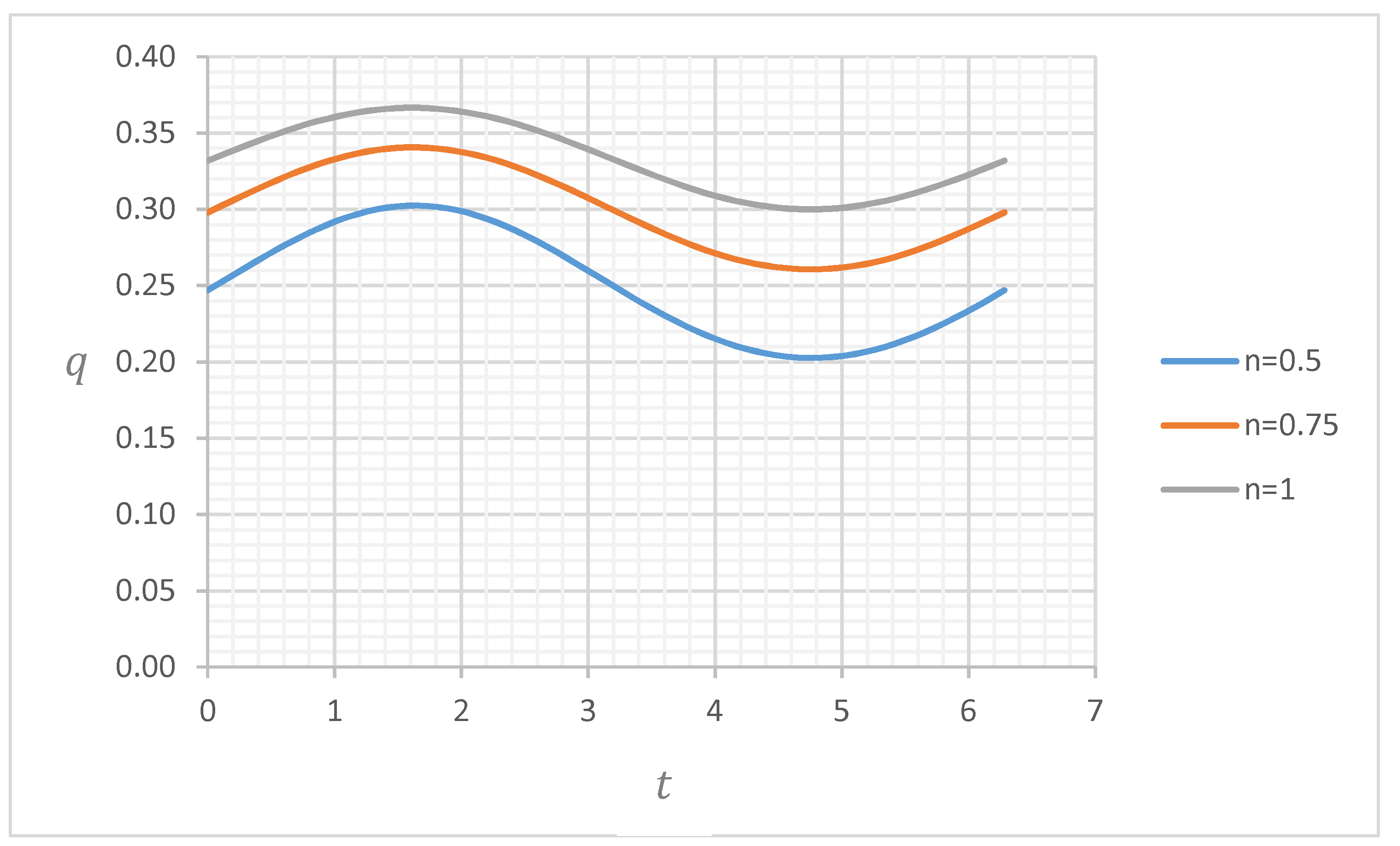
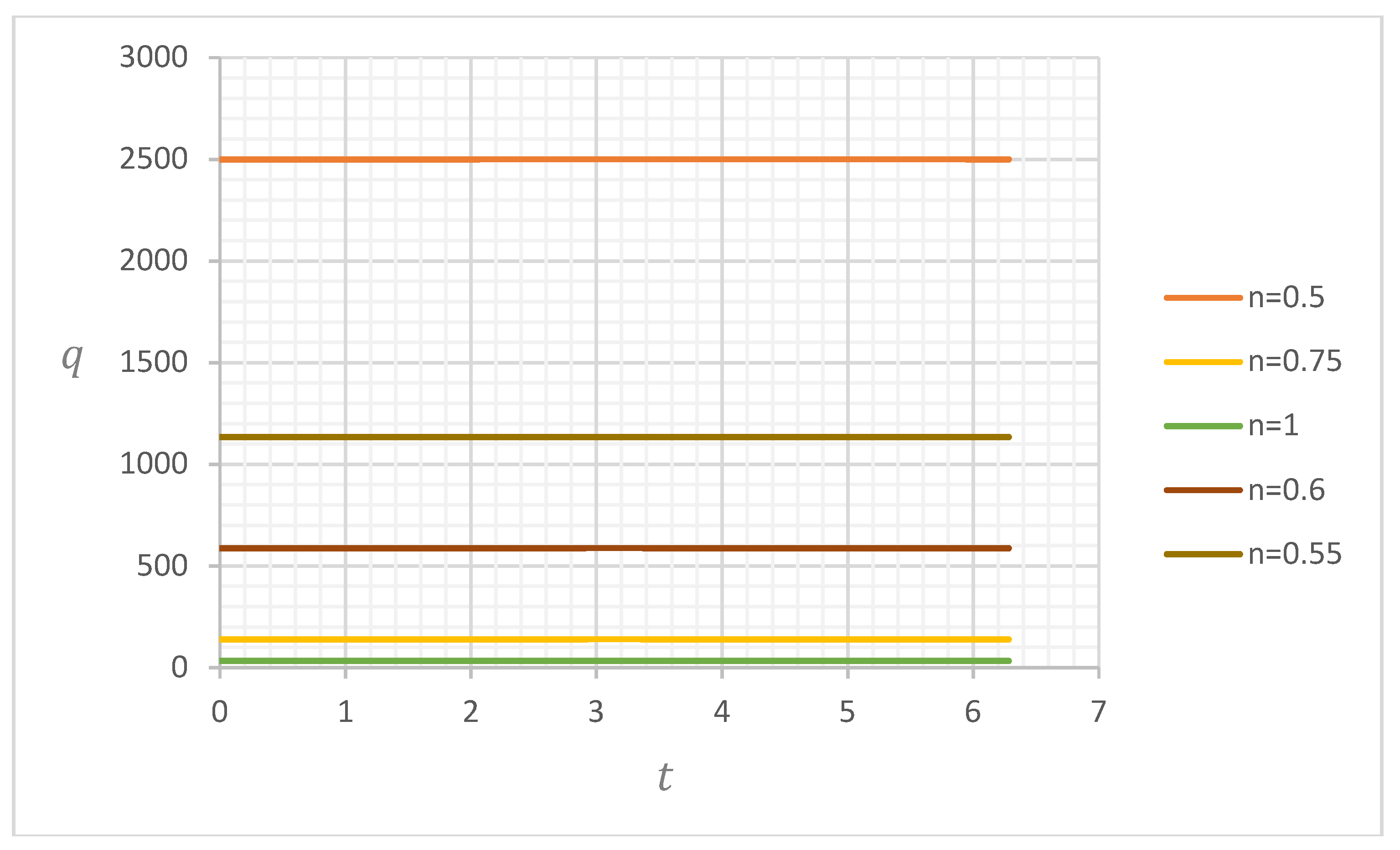
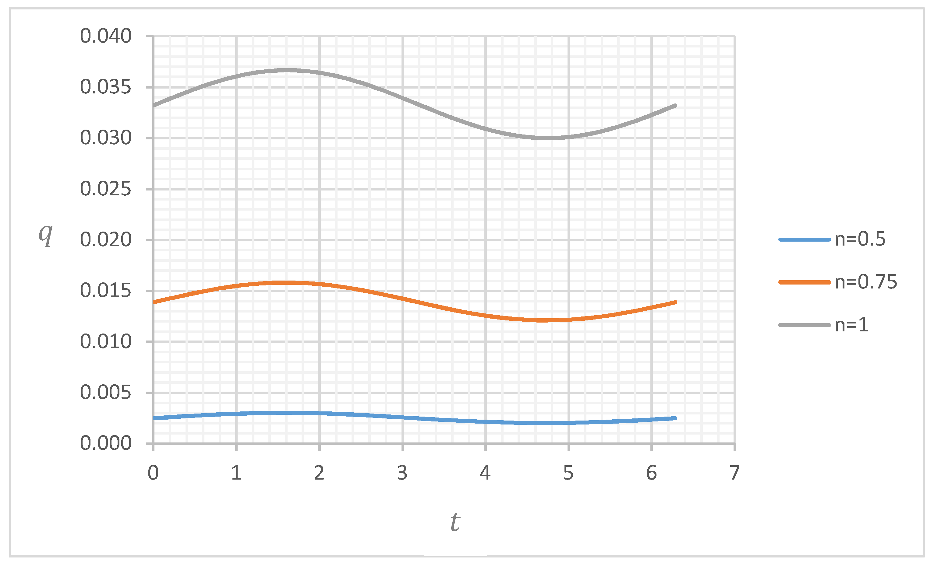
For small $Re$ and $\mathsf{\Omega }~1$, the term of order $\epsilon$ in Equation (52) could not be neglected, and the pulsation became important, with little influence of the flow index, as could be seen in Figure 6, where the three curves were practically coincident for $\mathsf{\Omega }=1,Re=0,1$ and $\epsilon =0.1$.

Figure 6. Wall shear stress for $\mathsf{\Omega }=1$, $Re=0.1$, $\epsilon =0.1$.

4.2. Discharge

The discharge was computed from Equations (52) to (56) and depended on $Re,\mathsf{\Omega }$, and $n$. For a given flow index, the following cases could be distinguished.

4.2.1. Discharge for $\mathsf{\Omega }\gg 1$ and $Re~1$

Equation (13) could be written as:

$$\frac{\partial u}{\partial t}=\frac{1}{\mathsf{\Omega }}+\frac{\epsilon }{\mathsf{\Omega }}\sin \left(t\right)+\frac{1}{\mathsf{\Omega }Re}\frac{\partial }{\partial y}\left({\left(\frac{\partial u}{\partial y}\right)}^n\right)$$

(69)

When Ω was large and $Re~1$, then $1/\mathsf{\Omega }\ll 1,\epsilon /\mathsf{\Omega }\ll 1$, and $1⁄\left(\mathsf{\Omega }Re\right)\ll 1$, resulting

$$\frac{\partial u}{\partial t}\ll 1$$

(70)

The above result indicated that the dependency of the velocity profile with time was negligible, from where no change of the discharge with time was expected. As an example, Figure 7 presents the discharge in function on time when $\mathsf{\Omega }=100,Re=1,\epsilon =0.1$ for $n=0.5,0.75$, and 1.

Figure 7. Discharge for $\mathsf{\Omega }=100$, $Re=1$, and $\epsilon =0.1$.

4.2.2. Discharge for $\mathsf{\Omega }\ll 1$ and $Re~1$

When Ω was small, the pulsating term was not negligible, and the fluctuation in time was noted in the discharge. Considering $\mathsf{\Omega }~\epsilon \ll 1$ resulted that the discharge was the superposition of the discharge for the steady-state condition with a fluctuating behaviour of the velocity given by $\mathsf{\Omega }\partial u/\partial t~\epsilon \sin \left(t\right)$, resulting in a harmonic oscillation of the discharge around the steady flow. As an example, Figure 8 shows the discharge for $\mathsf{\Omega }=0.1,Re=1,\epsilon =0.1$ for $n=0.5,0.75$, and 1.

Figure 8. Discharge for $\mathsf{\Omega }=0.1$, $Re=1$, and $\epsilon =0.1$.

4.2.3. Discharge for $\mathsf{\Omega }~1$ and $Re\gg 1$

Large $Re$ and $\mathsf{\Omega }~1$ mean large $\sigma$, and $q_1$ and $q_2$ tend to be negligible, and the discharge is defined by the steady part of the discharge, as in Equation (54). Figure 9 shows the discharge for $\mathsf{\Omega }=1,Re=100,\epsilon =0.1$ for several values of the flow index.

Figure 9. Discharge for $\mathsf{\Omega }=1$, $Re=100$, $\epsilon =0.1$.

4.2.4. Discharge for $\mathsf{\Omega }~1$ and $Re\ll 1$

When $\mathsf{\Omega }~1$ and $Re\ll 1$, the contributions of the unsteady components of the discharge became important and could not be neglected as in the previous case. As an example, Figure 10 shows the discharge for $\mathsf{\Omega }=1,Re=0.1,\epsilon =0.1$ for $n=0.5,0.75$.

Figure 10. Discharge for $\mathsf{\Omega }=1$, $Re=0.1$, $\epsilon =1$.

4.3. Flow Enhancement

The increment of discharge due to the non-linear behaviour of the constitutive law, summarized by $I_q$ (Equation (57)), is exemplified in Figure 11 and Figure 12. The first figure presents the flow enhancement for $n=0.75$ as function of the dimensionless frequency with the Reynolds number as a parameter. In Figure 12, for $Re=1$, the flow index was considered as a parameter. In both cases, $\epsilon =0.1$. As expected, at low frequencies, the discharge increment went to the value determined analytically. At large frequencies, there was no enhancement with respect to the non-pulsatile condition. Although the value of Ω, at which $I_q$ was nearly zero, increased with $Re$, the product $\mathsf{\Omega }Re$ remained nearly constant and was equal to 100. The same happened with the value of Ω at which the enhancement reached its maximum value. It decreased with $Re$, but $\mathsf{\Omega }Re\approx 0.1$. For a given $Re$, the Ω span, at which $I_q$ decreased from its maximum value to zero, was about 3 decades. As expected, the closer the fluid to a Newtonian behavior, the lower the flow enhancement, ($n\to 1,I_q\to 0$), as shown in Figure 12.

Figure 11. Dependency of the flow enhancement coefficient with dimensionless frequency and Reynolds number for $n=0.75$ and $\epsilon =0.1$.

Figure 12. Dependency of the flow enhancement coefficient with dimensionless frequency and flow index for $Re=1$ and $\epsilon =0.1$.

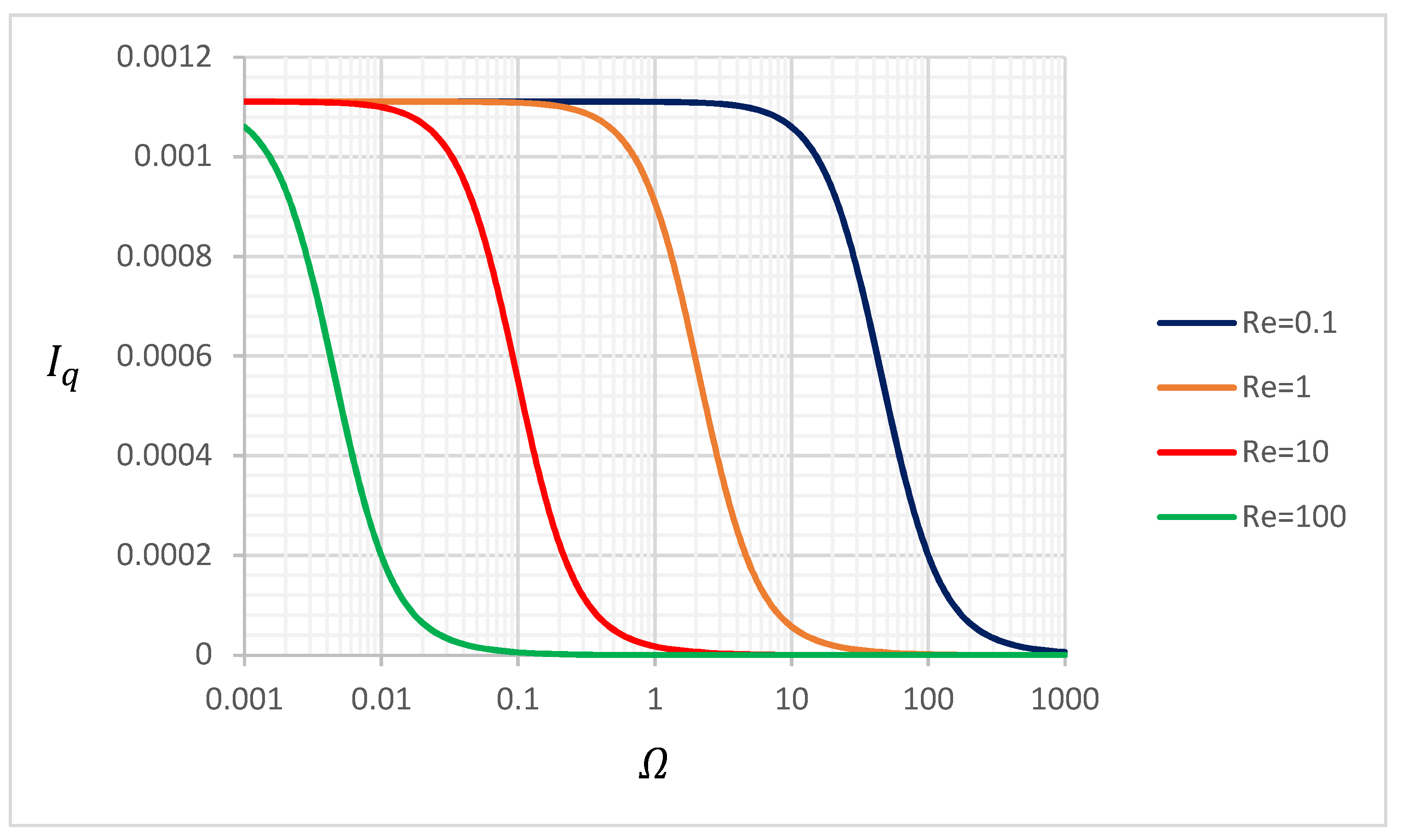
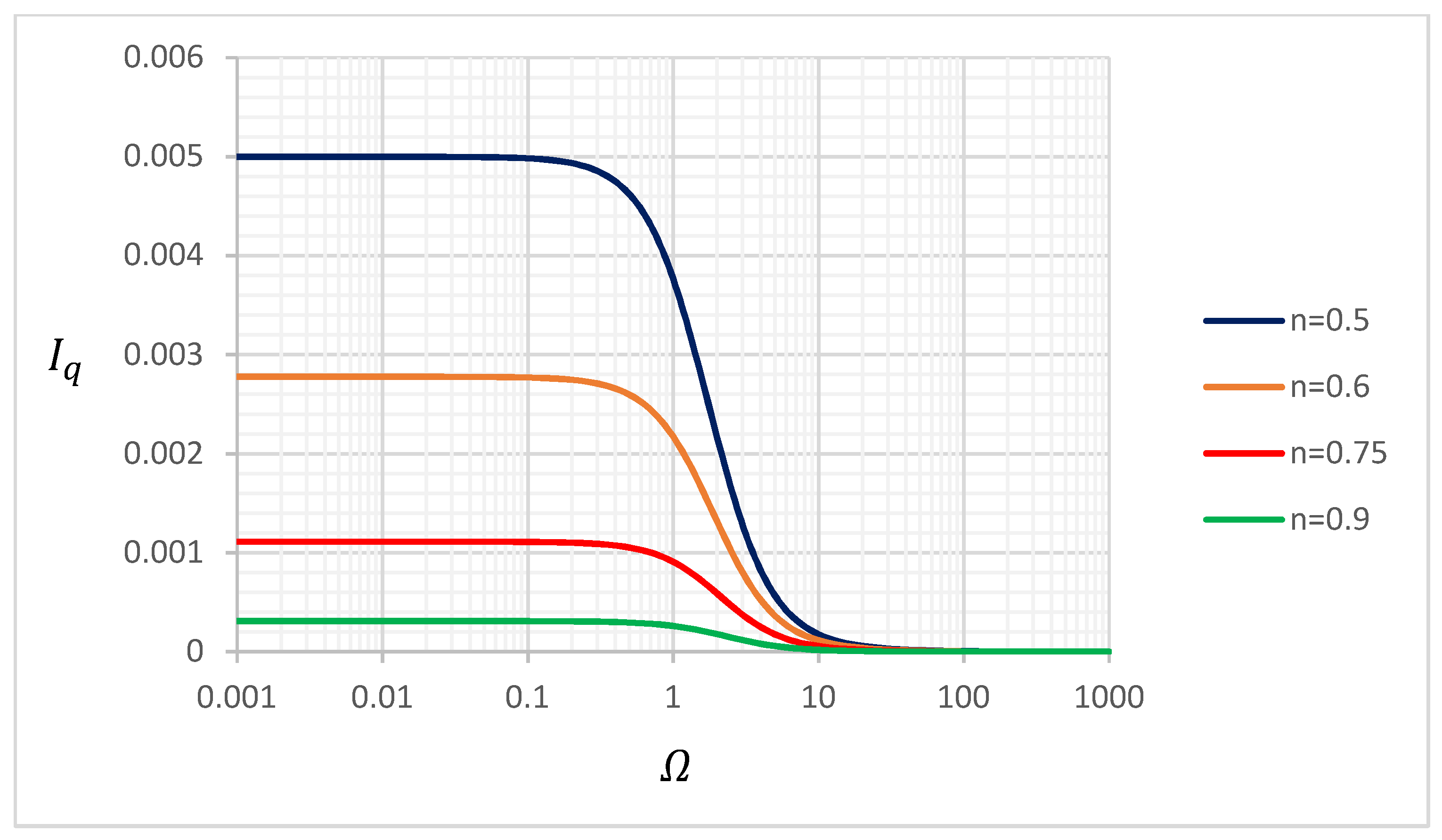
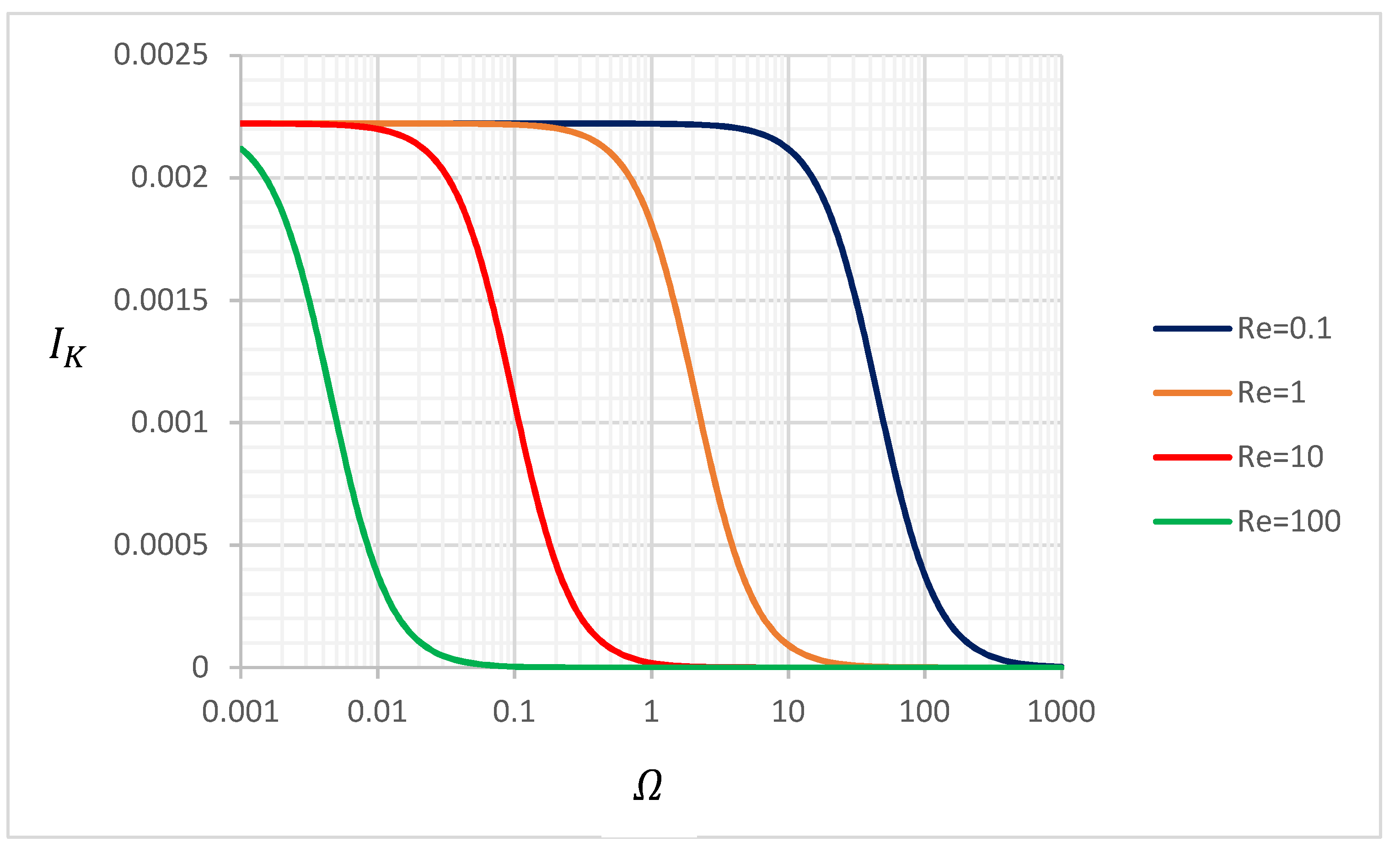
4.4. Dispersion Enhancement

The dispersion enhancement, characterized by $I_K$, behaved in an identical manner as $I_q$, as shown in Figure 13 and Figure 14, where the plots are for the same values of $Re$ and $n$ compared to in Figure 11 and Figure 12. Thus, it was observed that the dispersion enhancement goes to zero at a large dimensionless frequency as the pulsating pressure effect become negligible. For small frequencies, $I_K$ tend to a constant value. Like $I_q$, the range of Ω, at which $I_K$ decreases from its maximum value to zero, was around 3 decades, satisfying $\mathsf{\Omega }Re\approx 0.1$ for the maximum and $\mathsf{\Omega }Re\approx 100$ for zero, with $I_K\to 0$ as $n\to 1$ (Figure 14).

Figure 13. Dependency of the dispersion enhancement coefficient with dimensionless frequency and Reynolds numbers for $n=0.75$ and $\epsilon =0.1$.

Figure 14. Dependency of the dispersion enhancement coefficient with dimensionless frequency and flow index for $Re=1$ and $\epsilon =0.1$.

5. Conclusions

The pulsating two-dimensional flow of an Ostwald-de Waele fluid was solved analytically using the perturbation method up to the second-order term. Details of the analysis were presented, skipping only the more cumbersome algebra. A numerical solution based on spectral methods was also used to compute the velocity profile. Both analytical and numerical solutions showed very good agreement. From the velocity distribution, analytical expressions for the discharge and the wall shear stress were determined. The discharge and dispersion enhancements resulting from the nonlinearity of the rheology were also determined. These enhancements were noticed at the second-order. In terms of the dimensionless frequency, the enhancement coefficients behaved in a similar way for both the discharge and the dispersion coefficients, presenting a variation along 3 decades of Ω from their maximum values (corresponding to the non-inertial limit) to zero (for the non-pulsatile condition).

References

- Sexl, T.; Ueber den von, E.G. Richardson entdeckten Annulareffect. Z. Phys. 1930, 61, 349–362. [Google Scholar] [CrossRef]
- Lambossy, P. Oscillations forcees d’un liquide incompressible et visqueux dans un tuve rigide et horizontal. Calcul de la force de frottement. Helv. Phys. Acta 1952, 25, 371–386. [Google Scholar]
- Womersley, J. Method for the calculation of velocity, rate of flow and viscous drag in arteries when the pressure gradient is known. J. Physiol. 1955, 127, 553–563. [Google Scholar] [CrossRef] [PubMed]
- Womersley, J. Oscillatory motion of a viscous liquid in a thin-walled elastic tube-I: The linear approximation for long waves. Proc. R. Soc. Ser. 1955, 46, 199–221. [Google Scholar] [CrossRef]
- Pipkin, A.C. Alternating flow of non-Newtonian Fluids in tubes of arbitrary cross-section. Arch. Rat. Mech. Anal. 1964, 15, 1–13. [Google Scholar] [CrossRef]
- Etter, I.; Schowalter, W.R. Unsteady flow of an Oldroyd fluid in a circular tube. Trans. Soc. Rheol. 1965, 9, 351–369. [Google Scholar] [CrossRef]
- Rahaman, K.D.; Ramkissoon, H. Unsteady axial viscoelastic pipe flows. J. Non Newton. Fluid Mech. 1995, 57, 27–38. [Google Scholar] [CrossRef]
- Uchida, S. Pulsating viscous flow superposed on the steady laminar motion. Z. Angew. Math. Phys.(ZAMP) 1956, 5, 403–422. [Google Scholar] [CrossRef]
- Barnes, H.A.; Townsend, P.; Walters, K. On pulsatile flow of non-Newtonian liquids. Rheol. Acta 1971, 10, 517–527. [Google Scholar] [CrossRef]
- Phan-Thien, N.; Dudek, J. Pulsating flow revisited. J. Non Newton. Fluid Mech. 1982, 11, 147–161. [Google Scholar] [CrossRef]
- Phan-Thien, N. Flow enhancement mechanisms of a pulsating flow of non-Newtonian liquids. Rheol. Acta 1980, 19, 285–290. [Google Scholar] [CrossRef]
- Steller, R. A new approach to the pulsating oscillating flows of viscoelastic liquid in channels. Rheol. Acta 1993, 32, 192–205. [Google Scholar] [CrossRef]
- Davies, J.M.; Bhumiratana, S.; Bird, R.B. Elastic and inertial effects in pulsatile flow of polymeric liquids in circular tubes. J. Non Newton. Fluid Mech. 1978, 3, 237–259. [Google Scholar] [CrossRef]
- Mai, T.-Z.; Davis, A.M.J. Laminar pulsatile two-phase non-Newtonian flow through a pipe. Comput. Fluids 1996, 25, 77–93. [Google Scholar] [CrossRef]
- Daprà, I.; Scarpi, G. Pulsatile pipe flow of pseudoplastic fluids. Meccanica 2006, 41, 501–508. [Google Scholar] [CrossRef]
- Merril, E.W. Rheology of blood. Physiol. Rev. 1969, 49, 863–888. [Google Scholar]
- Prakash, J.; Ogulu, A. A study of pulsatile blood flow modelled as a power law fluid in a constricted tube. Int. Commun. Heat Mass. Transfer. 2007, 34, 762–768. [Google Scholar] [CrossRef]
- Sankar, D.S.; Lee, U. Mathematical modelling of pulsatile flow of non-Newtonian fluid in stenosed arteries. Commun. Nonlinear Sci. Numer. Simulat. 2009, 14, 2971–2981. [Google Scholar] [CrossRef]
- Herrera-Valencia, E.E.; Calderas, F.; Medina-Torres, L.; Pérez-Camacho, M.; Moreno, L.; Manero, O. On the pulsating flow behavior of a biological fluid: Human blood. Rheol. Acta 2017, 56, 387–407. [Google Scholar] [CrossRef]
- Siginer, A. On the pulsating pressure gradient driven flow of viscoelastic liquids. J. Rheol. 1991, 35, 271–311. [Google Scholar] [CrossRef]
- McGInty, S.; McKee, S.; McDermont, R. Analytic solutions of Newtonian and non-Newtonian pipe flows subject to a general time-dependent pressure gradient. J. Non Newton. Fluid Mech. 2009, 162, 54–77. [Google Scholar] [CrossRef]
- Daprà, I.; Scarpi, G. Pulsatile Poiseuille flow of a viscoplastic fluid in the gap between coaxial cylinders. J. Fluids Eng. 2011, 133, 081203. [Google Scholar] [CrossRef]
- Letelier, M.F.; Siginer, D.A.; Caceres, C. Pulsating flow of viscoelastic fluids in straight tubes of arbitrary cross-section—Part I: Longitudinal Field. Int. J. Non Linear Mech. 2002, 37, 369–393. [Google Scholar] [CrossRef]
- Daprà, I.; Scarpi, G. Perturbation solution for pulsatile flow of a non-Newtonian Williamson fluid in a rock fracture. Int. J. Rock Mech. Min. Sci. 2007, 44, 271–278. [Google Scholar] [CrossRef]
- Nandakumar, N.; Sahu, K.C.; Anand, M. Pulsatile flow of a shear thinning model for blood through a two-dimensional stenosed channel. Eur. J. Mech. B Fluids 2015, 49, 29–35. [Google Scholar] [CrossRef]
- Edwards, M.F.; Nellist, D.A.; Wilkinson, W.L. Unsteady, laminar flows of non-Newtonian fluids in pipes. Chem. Eng. Sci. 1972, 27, 295–306. [Google Scholar] [CrossRef]
- Balmer, R.T.; Fiorina, M.A. Unsteady flow of an inelastic power law fluid in a circular tube. J. Non Newton. Fluid Mech. 1980, 7, 89–198. [Google Scholar] [CrossRef]
- Adusumilli, R.S.; Hill, G.A. Transient Laminar Flows of Truncated Power Law Fluids in Pipes. Can. J. Chem. Eng. 1984, 62, 594–601. [Google Scholar] [CrossRef]
- Nakamura, M.; Sawada, T. Numerical study on the laminar pulsatile flow of slurries. J. Non Newton. Fluid Mech. 1987, 22, 191–206. [Google Scholar] [CrossRef]
- Warsi, Z.U.A. Unsteady flow of power-law fluids through circular pipes. J. Non Newton. Fluid Mech. 1994, 55, 197–202. [Google Scholar] [CrossRef]
- Javadzadegan, A.; Esmaeili, M.; Majidi, S.; Fakhimghanbarzadeh, B. Pulsatile flow of viscous and viscoelastic fluids in constricted tubes. J. Mech. Sci. Technol. 2009, 23, 2456–2467. [Google Scholar] [CrossRef]
- Yakhot, A.; Arad, M.; Ben-Dor, G. Numerical investigation of a laminar pulsating flow in a rectangular duct. Int. J. Numer. Meth. Fluids 1999, 29, 935–950. [Google Scholar] [CrossRef]
- Tu, C.; Deville, M. Pulsatile flow of non-newtonian fluids through arterial stenoses. J. Biomech. 1996, 29, 899–908. [Google Scholar] [CrossRef]
- Pontrelli, G. Pulsatile blood flow in a pipe. Comput. Fluids 1998, 27, 367–380. [Google Scholar] [CrossRef][Green Version]
- Harris, J.; Maheshwari, R. Oscillatory pipe flow: A comparison between predicted and observed displacement profiles. Rheol. Acta 1975, 14, 162–168. [Google Scholar] [CrossRef]
- Thurston, G. Elastic Effects in Pulsatile Blood Flow. Microvasc. Res. 1975, 9, 145–157. [Google Scholar] [CrossRef]
- Davies, J.; Chakrabarti, A. A modified pulsatile flow apparatus for measuring flow enhancement in combined steady and oscillatory shear flow. In Rheology, 1st ed.; Astarita, G., Marruci, G., Nicolais, L., Eds.; Springer Science + Business Media: New York, NY, USA, 1980. [Google Scholar]
- Kajiuchi, T.; Saito, A. Flow enhancement of laminar pulsating flow of Bingham plastic fluids. J. Chem. Eng. Jpn. 1984, 17, 34–38. [Google Scholar] [CrossRef]
- Lin, Y.; Tan, G.; Phan-Thien, N.; Khoo, B. Flow enhancement in pulsating flow of non-colloidal suspensions in tubes. J. Non Newton. Fluid Mech. 2014, 212, 13–17. [Google Scholar] [CrossRef]
- Watson, G. A Treatise on the Theory of Bessel Functions, 1st ed.; Cambridge University Press: Cambridge, UK, 1922. [Google Scholar]
- Fischer, H.B.; List, E.J.; Koh, R.Y.; Imberger, J.; Brooks, N.H. Mixing in Inland and Coastal Waters; Academic Press Inc.: Cambridge, MA, USA, 1979. [Google Scholar]
- Thomas, G.; Finney, R. Calculus and Analytic Geometry, 9th ed.; Addison-Wesley: Boston, MA, USA, 1996. [Google Scholar]
- Patera, A.T. A spectral element method for fluid dynamics: Laminar flow in a channel expansion. J. Comput. Phys. 1984, 54, 468–488. [Google Scholar] [CrossRef]
- Kim, J.; Moin, P.; Moser, R. Turbulence statistics in fully developed channel flow at low Reynolds number. J. Fluid Mech. 1987, 177, 133–166. [Google Scholar] [CrossRef]
- Manna, M.; Vacca, A.; Deville, M. Preconditioned spectral multi-domain discretization of the incompressible Navier-Stokes equations. J. Comp. Phys. 2004, 201, 204–223. [Google Scholar] [CrossRef]
- Huang, L.; Chen, Q. Spectral Collocation Model for Solitary Wave Attenuation and Mass Transport over Viscous Mud. J. Eng. Mech. 2009, 135, 881–891. [Google Scholar] [CrossRef]
- Liu, R.; Liu, Q.S. Non-modal instability in plane Couette flow of a power-law fluid. J. Fluid Mech. 2011, 676, 145–171. [Google Scholar] [CrossRef]
- Niu, J.; Zheng, L.; Yang, Y.; Shu, C.-W. Chebyshev spectral method for unsteady axisymmetric mixed convection heat transfer of power law fluid over a cylinder with variable transport properties. Int. J. Numer. Anal. Mod. 2014, 11, 525–540. [Google Scholar]
- Canuto, C.; Hussaini, M.; Quarteroni, A.; Zang, T. Spectral Methods in Fluid Dynamics; Springer: Berlin/Heidelberg, Germany, 1988. [Google Scholar]
- Manna, M.; Vacca, A. An efficient method for the solution of the incompressible Navier-Stokes equations in cylindrical geometries. J. Comput. Phys. 1999, 151, 563–584. [Google Scholar] [CrossRef]
- Pascal, J.P.; D’Alessio, J.D.; Hasan, M. Instability of gravity-driven flow of a heated power-law fluid with temperature dependent consistency. AIP Adv. 2018, 8, 105215–105226. [Google Scholar] [CrossRef]
- Iervolino, M.; Pascal, J.P.; Vacca, A. Instabilities of a power–law film over an inclined permeable plane: A two–sided model. J. Non Newton. Fluid Mech. 2018, 259, 111–124. [Google Scholar] [CrossRef]
- Iervolino, M.; Pascal, J.P.; Vacca, A. Thermocapillary instabilities of a shear-thinning fluid falling over a porous layer. J. Non Newton. Fluid Mech. 2019, 270, 36–50. [Google Scholar] [CrossRef]
© 2020 by the authors. Licensee MDPI, Basel, Switzerland. This article is an open access article distributed under the terms and conditions of the Creative Commons Attribution (CC BY) license (http://creativecommons.org/licenses/by/4.0/).