Estimation of Yield Response Factor for Each Growth Stage under Local Conditions Using AquaCrop-OS

 ,
,  , ,
, ,  , and
, and 
Abstract
1. Introduction
2. Methodology
2.1. Crop Yield Equation
2.2. Estimation of Using AquaCrop-OS
2.3. Case Study
2.4. Model Inputs
3. Results and Discussions
3.1. Yield Response Factor for Each Growth Stage
3.1.1. Yield Response Factor For Maize
3.1.2. Yield Response Factor for Sugar Beet
3.1.3. Yield Response Factor For Wheat
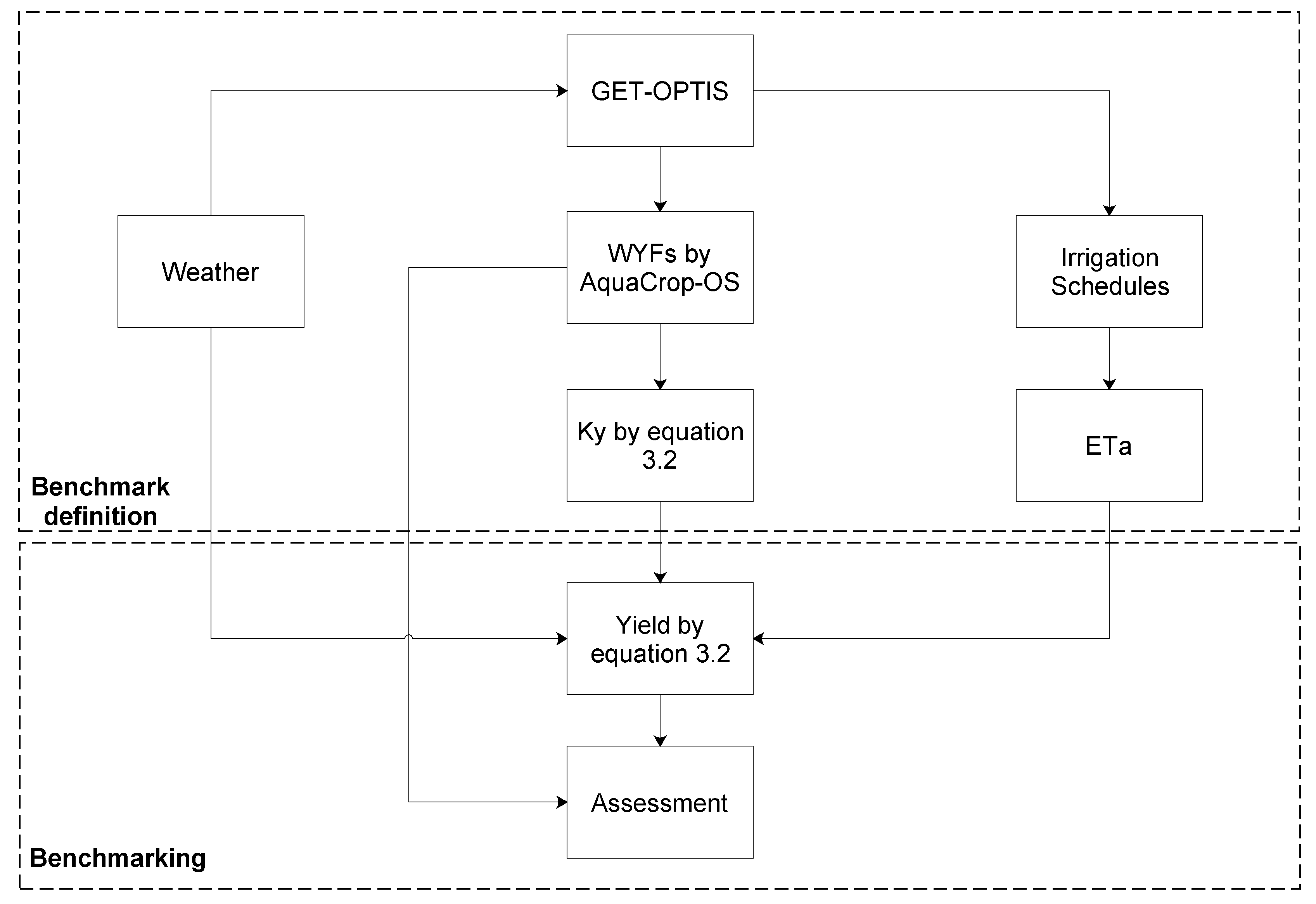
3.2. Benchmarking of the Proposed Methodology
3.2.1. Benchmarking for a Specific Year
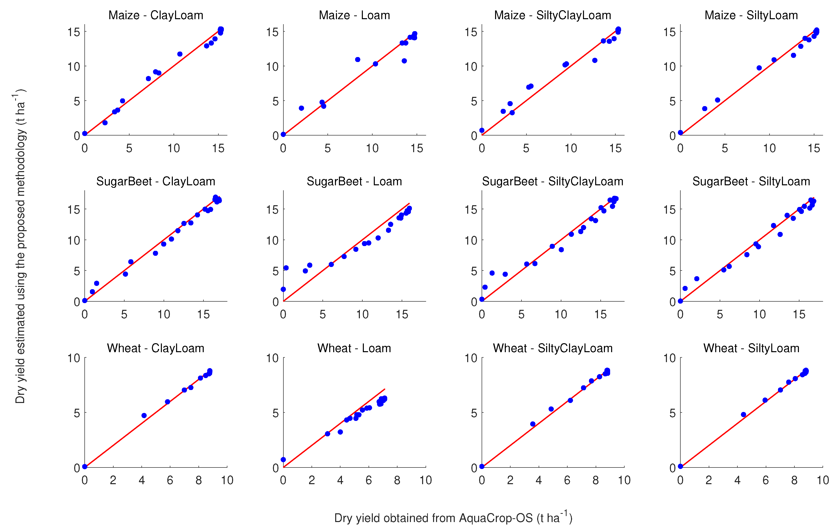
3.2.2. Benchmarking for All Years
4. Conclusions
Author Contributions
Funding
Acknowledgments
Conflicts of Interest
References
- FAO. AQUASTAT Website. FAO’s Information System on Water and Agriculture; Food and Agriculture Organization of the United Nations: Rome, Italy, 2016. [Google Scholar]
- Hubick, K.T.; Farquhar, G.D.; Shorter, R. Correlation between water use efficiency and carbon isotope discrimination in diverse peanut (Arachis) germplasm. Aust. J. Plant Physiol. 1986, 13, 803–816. [Google Scholar] [CrossRef]
- Saccon, P. Water for agriculture, irrigation management. Appl. Soil Ecol. 2017. [Google Scholar] [CrossRef]
- Malik, A.; Shakir, A.; Ajmal, M.; Khan, M.; Khan, T. Assessment of AquaCrop model in simulating sugar beet canopy cover, biomass and root yield under different irrigation and field management practices in semi-arid regions of Pakistan. Water Resour. Manag. 2017, 31, 4275–4292. [Google Scholar] [CrossRef]
- Steduto, P.; Hsiao, T.; Raes, D.; Fereres, E. AquaCrop—The FAO crop model to simulate yield response to water: I. Concepts and underlying principles. Agron. J. 2009, 101, 426–437. [Google Scholar] [CrossRef]
- Paredes, P.; de Melo-Abreu, J.; Alves, I.; Pereira, L.S. Assessing the performance of the FAO AquaCrop model to estimate maize yields and water use under full and deficit irrigation with focus on model parameterization. Agric. Water Manag. 2014, 144, 81–97. [Google Scholar] [CrossRef]
- Nyakudya, I.W.; Stroosnijder, L. Effect of rooting depth, plant density and planting date on maize (Zea mays L.) yield and water use efficiency in semi-arid Zimbabwe: Modeling with AquaCrop. Agric. Water Manag. 2014, 146, 280–296. [Google Scholar] [CrossRef]
- Heng, L.K.; Hsiao, T.; Evett, S.; Howell, T.; Steduto, P. Validating the FAO AquaCrop model for irrigated and water deficient field maize. Agron. J. 2009, 101, 488–498. [Google Scholar] [CrossRef]
- Toumi, J.; Er-Raki, S.; Ezzahar, J.; Khabba, S.; Jarlan, L.; Chehbouni, A. Performance assessment of AquaCrop model for estimating evapotranspiration, soil water content and grain yield of winter wheat in Tensift Al Haouz (Morocco): Application to irrigation management. Agric. Water Manag. 2016, 163, 219–235. [Google Scholar] [CrossRef]
- Mkhabela, M.S.; Paul, R.B. Performance of the FAO AquaCrop model for wheat grain yield and soil moisture simulation in Western Canada. Agric. Water Manag. 2012, 110, 16–24. [Google Scholar] [CrossRef]
- Andarzian, B.; Bannayan, M.; Steduto, P.; Mazraeh, H.; Barati, M.E.; Barati, M.A.; Rahnama, A. Validation and testing of the AquaCrop model under full and deficit irrigated wheat production in Iran. Agric. Water Manag. 2011, 100, 1–8. [Google Scholar] [CrossRef]
- Alishiri, R.; Paknejad, F.; Aghayari, F. Simulation of sugarbeet growth under different water regimes and nitrogen levels by AquaCrop. Int. J. Biosci. 2014, 4, 1–9. [Google Scholar]
- Stricevic, R.; Cosic, M.; Djurovic, N.; Pejic, B.; Maksimovic, L. Assessment of the FAO AquaCrop model in the simulation of rainfed and supplementally irrigated maize, sugar beet and sunflower. Agric. Water Manag. 2011, 98, 1615–1621. [Google Scholar] [CrossRef]
- Montoya, F.; Camargo, D.; Ortega, J.; Córcoles, J.; Domínguez, A. Evaluation of AquaCrop model for a potato crop under different irrigation conditions. Agric. Water Manag. 2016, 164, 267–280. [Google Scholar] [CrossRef]
- Garcia-Vila, M.; Fereres, E. Combining the simulation crop model AquaCrop with an economic model for the optimization of irrigation management at farm level. Eur. J. Agron. 2012, 36, 21–31. [Google Scholar] [CrossRef]
- Araya, A.; Habtu, S.; Hagdu, K.M.; Kebede, A.; Dejene, T. Test of AquaCrop model in simulating biomass and yield of water deficient and irrigated barley (Hordeum vulgare). Agric. Water Manag. 2010, 97, 1838–1846. [Google Scholar] [CrossRef]
- Geerts, S.; Raes, D.; Garcia, M.; Miranda, R.; Cusicanqui, J.A.; Taboada, C.; Mendoza, J.; Huanca, R.; Mamani, A.; Condori, O.; et al. Simulating yield response of quinoa to water availability with AquaCrop. Agron. J. 2009, 101, 499–508. [Google Scholar] [CrossRef]
- Maniruzzaman, M.; Talukder, M.S.U.; Khan, M.H.; Biswas, J.C.; Nemes, A. Validation of the AquaCrop model for irrigated rice production under varied water regimes in Bangladesh. Agric. Water Manag. 2015, 159, 331–340. [Google Scholar] [CrossRef]
- Jensen, J. Water consumption by agricultural plants. In Water Deficit and Plant Growth; Kozlowski, T., Ed.; Academic Press: New York, NY, USA, 1968; pp. 1–22. [Google Scholar]
- Doorenbos, J.; Kassam, A. Yield Response to Water; FAO: Rome, Italy, 1979. [Google Scholar]
- Carvallo, H.O.; Holzapfel, E.A.; Lopez, M.A.; Mariño, M.A. Irrigated cropping optimization. J. Irrig. Drain. Engin. ASCE 1998, 124, 67–72. [Google Scholar] [CrossRef]
- Kipkorir, E.; Sahli, A.; Raes, D. MIOS: A decision tool for determination of optimal irrigated cropping pattern of a multicrop system under water scarcity constraints. Irrig. Drain. 2002, 51, 155–166. [Google Scholar] [CrossRef]
- Raes, D.; Geerts, S.; Kipkorir, E.; Wellens, J.; Sahli, A. Simulation of yield decline as a result of water stress with a robust soil water balance model. Agric. Water Manag. 2006, 81, 335–357. [Google Scholar] [CrossRef]
- Schütze, N.; de Paly, M.; Shamir, U. Novel simulation-based algorithms for optimal open-loop and closed-loop scheduling of deficit irrigation systems. J. Hydroinform. 2012, 14, 136–151. [Google Scholar] [CrossRef]
- Singh, A. Optimal Allocation of Resources for the Maximization of Net Agricultural Return. J. Irrig. Drain. Eng. 2012, 138, 830–836. [Google Scholar] [CrossRef]
- Banihabib, M.; Zahraei, A.; Eslamian, S. Dynamic programming model for the system of a non-uniform deficit irrigation and reservoir. Irrig. Drain. 2017, 66, 71–81. [Google Scholar] [CrossRef]
- Kuschel-Otárola, M.; Rivera, D.; Holzapfel, E.; Palma, C.D.; Godoy-Faúndez, A. Multiperiod optimisation of irrigated crops under different conditions of water availability. Water 2018, 10, 1434. [Google Scholar] [CrossRef]
- Steduto, P.; Hsiao, T.C.; Fereres, E.; Raes, D. Crop Yield Response to Water. FAO Irrigation and Drainage Paper 66; Food and Agriculture Organization of the United Nations: Rome, Italy, 2012; p. 503. [Google Scholar]
- Karamouz, M.; Zahraie, B.; Kerachian, R.; Eslami, A. Crop pattern and conjuctive use management: A case study. Irrig. Drain. 2010, 59, 161–173. [Google Scholar] [CrossRef]
- Shrestha, N.; Geerts, S.; Raes, D.; Horemans, S.; Soentjens, S.; Maupas, F.; Clouet, P. Yield response of sugar beets to water stress under Western European conditions. Agric. Water Manag. 2010, 97, 346–350. [Google Scholar] [CrossRef]
- Kresović, B.; Tapanarova, A.; Tomić, Z.; Životić, L.; Vujović, D.; Sredojević, Z.; Gajić, B. Grain yield and water use efficiency of maize as influenced by different irrigation regimes through sprinkler irrigation under temperate climate. Agric. Water Manag. 2016, 169, 34–43. [Google Scholar] [CrossRef]
- Djaman, K.; Irmak, S.; Rathje, W.R.; Martin, D.L.; Eisenhauer, D.E. Maize evapotranspiration, yield production function, biomass, grain yield, harvest index, and yield response factors under full and limited irrigation. Trans. ASABE 2013, 56, 273–293. [Google Scholar]
- Kiymaz, S.; Ertek, A. Yield and quality of sugar beet (Beta vulgaris L.) at different water and nitrogen levels under the climatic conditions of Kirsehir, Turkey. Agric. Water Manag. 2015, 158, 156–165. [Google Scholar] [CrossRef]
- Tarkalson, D.D.; King, B.A.; Bjorneberg, D.L. Yield production functions of irrigated sugarbeet in an arid climate. Agric. Water Manag. 2018, 200, 1–9. [Google Scholar] [CrossRef]
- Bandyopadhyay, K.K.; Misra, A.K.; Ghosh, P.K.; Hati, K.M.; Mandal, K.G.; Moahnty, M. Effect of irrigation and nitrogen application methods on input use efficiency of wheat under limited water supply in a Vertisol of Central India. Irrig. Sci. 2010, 28, 285–299. [Google Scholar] [CrossRef]
- Liu, X.W.; Shao, L.W.; Sun, H.Y.; Chen, S.Y.; Zhang, X.Y. Responses of yield and water use efficiency to irrigation amount decided by pan evaporation for winter wheat. Agric. Water Manag. 2013, 129, 173–180. [Google Scholar] [CrossRef]
- Foster, T.; Brozovic, N.; Butler, A.; Neale, C.; Raes, D.; Steduto, P.; Fereres, E.; Hsiao, T. AquaCrop-OS: An open source version of FAO’s crop water productivity model. Agric. Water Manag. 2017, 181, 18–22. [Google Scholar] [CrossRef]
- MathWorks. Parallel Computing Toolbox: User’s Guide; Technical Report; The MathWorks, Inc.: Natick, MA, USA, 2017. [Google Scholar]
- Raes, D.; Steduto, P.; Hsiao, T.C.; Fereres, E. Reference Manual: AquaCrop Plug-in Program (Version 4.0); Technical Report; FAO: Rome, Italy, 2012. [Google Scholar]
- Loague, K.; Green, R.E. Statistical and graphical methods for evaluating solute transport models; overview and application. J. Contam. Hydrol. 1991, 7, 51–73. [Google Scholar] [CrossRef]
- Jamieson, P.D.; Porter, J.R.; Wilson, D.R. A test of the computer simulation model ARC-WHEAT1 on wheat crops grown in New Zealand. Field Crop. Res. 1991, 27, 337–350. [Google Scholar] [CrossRef]
- DGA. Diagnóstico y Clasificación de los Cursos y Cuerpos de Agua Según Objetivo y Calidad; Cuenca del río Itata: Santiago, Chile, 2004. [Google Scholar]
- ODEPA. Región del Biobío: Información Regional 2018; Technical Report; Oficina de Estudios y Políticas Agrarias (ODEPA): Santiago, Chile, 2018. [Google Scholar]
- Rivera, D.; Granda, S.; Arumí, J.L.; Sandoval, M.; Billib, M. A methodology to identify representative configurations of sensors for monitoring soil moisture. Environ. Monit. Assess. 2011, 184, 6563–6574. [Google Scholar] [CrossRef]
- Granda, S.; Rivera, D.; Arumí, J.L.; Sandoval, M. Monitoreo continuo de humedad con fines hidrológicos. Tecnolog. Cienc. Agua 2013, 4, 189–197. [Google Scholar]
- Rivera, D.; Sandoval, M.; Godoy, A. Exploring soil databases: A self-organizing map approach. Soil Use Manag. 2015, 31, 121–131. [Google Scholar] [CrossRef]
- Faiguenbaum, H. Labranza, Siembra y Producción de los Principales Cultivos de Chile; Vivaldi y Asociados: Santiago, Chile, 2003; p. 760. [Google Scholar]
- Allen, R.G.; Walter, I.A.; Elliott, R.; Itenfisu, D.; Brown, P.; Jensen, M.E.; Mecham, B.; Howell, T.A.; Snyder, R.; Eching, S.; et al. Task Committee on Standardization of Reference Evapotranspiration; SCE: Reston, VA, USA, 2005. [Google Scholar]
- Van Genuchten, M.T.; Leij, F.J.; Yates, S.R. The RETC Code for Quantifying the Hydraulic Functions of Unsaturated Soils; EPA/600/2-91/065; U.S. Environmental Protection Agency: Ada, OK, USA, 1991; p. 85.
- Kuschel-Otárola, M. Estimación de Flujos de Agua en un Andisol Usando Datos de Humedad. Bachelor’s Thesis, Universidad de Concepción, Chillán, Chile, 2014. [Google Scholar]
- FAO. “CROPWAT 8.0” Databases and Software; FAO: Rome, Italy, 2017. [Google Scholar]


| Parameter | Crop | ||
|---|---|---|---|
| Maize | Sugar Beet | Wheat | |
| Conservative (generally applicable) | |||
| Base temperature (C) | 8.00 | 5.00 | 0.00 |
| Cut-off temperature (C) | 30.00 | 30.00 | 26.00 |
| Canopy cover per seedling at 90% emergence (CCo) | 6.50 | 1.00 | 1.50 |
| Canopy growth coefficient (CGC) | 1.25 | 1.05 | 0.50 |
| Maximum canopy cover (CCx) | 96.00 | 98.00 | 96.00 |
| Crop coefficient for transpiration at CC = 100% | 1.05 | 1.10 | 1.10 |
| Decline in crop coef. after reaching CCx | 0.30 | 0.15 | 0.15 |
| Canopy decline coefficient (CDC) at senescence | 1.00 | 0.39 | 0.40 |
| Water productivity, normalised to the year 2000 (WP*) | 33.70 | 17.00 | 15.00 |
| Leaf growth threshold (Pupper) | 0.14 | 0.20 | 0.20 |
| Leaf growth threshold (Plower) | 0.72 | 0.60 | 0.65 |
| Leaf growth stress coefficient curve shape | 2.90 | 3.00 | 5.00 |
| Stomatal conductance threshold (Pupper) | 0.69 | 0.65 | 0.65 |
| Stomata stress coefficient curve shape | 6.00 | 3.00 | 2.50 |
| Senescence stress coefficient (Pupper) | 0.69 | 0.75 | 0.70 |
| Senescence stress coefficient curve shape | 2.70 | 3.00 | 2.50 |
| Considered to be conservative but can or may be cultivar-specific | |||
| Reference harvest index (HIo) | 48 | 70 | 48 |
| GDD from 90% emergence to start of anthesis | 800 | 842 | 1100 |
| Duration of anthesis, in GDD | 180 | 0 | 200 |
| Coefficient, inhibition of leaf growth on HI | 7 | 4 | 10 |
| Coefficient, inhibition of stomata on HI | 3 | - | 7 |
| Maximum yield (t ha−1) (more details in Kuschel-Otárola et al. [27]) | 15 | 100 | 7 |
| Sand | Silt | Clay | ||||||
|---|---|---|---|---|---|---|---|---|
| Soil | (%) | (g cm−3) | (m3 m−3) | (mm day−1) | ||||
| ClayLoam 1 | 22 | 48 | 30 | 0.72 | 0.73 | 0.45 | 0.30 | 3415.9 |
| ClayLoam 2 | 35 | 38 | 27 | 0.97 | 0.64 | 0.57 | 0.33 | 269.1 |
| ClayLoam 3 | 39 | 28 | 33 | 1.39 | 0.47 | 0.34 | 0.26 | 132.4 |
| Loam 1 | 34 | 42 | 24 | 0.71 | 0.73 | 0.44 | 0.28 | 3517.8 |
| Loam 2 | 31 | 46 | 23 | 1.07 | 0.60 | 0.59 | 0.40 | 69.5 |
| Loam 3 | 41 | 37 | 22 | 1.13 | 0.57 | 0.55 | 0.34 | 110.3 |
| SiltyClayLoam 1 | 10 | 52 | 38 | 0.78 | 0.70 | 0.46 | 0.32 | 2382.0 |
| SiltyClayLoam 2 | 11 | 52 | 37 | 0.81 | 0.69 | 0.50 | 0.32 | 1903.3 |
| SiltyClayLoam 3 | 15 | 49 | 36 | 0.86 | 0.68 | 0.50 | 0.36 | 1534.2 |
| SiltyLoam 1 | 27 | 50 | 23 | 0.71 | 0.73 | 0.44 | 0.28 | 3571.7 |
| SiltyLoam 2 | 22 | 51 | 27 | 0.98 | 0.63 | 0.59 | 0.38 | 183.9 |
| SiltyLoam 3 | 24 | 51 | 25 | 1.03 | 0.61 | 0.59 | 0.44 | 76.3 |
| Crop | Soil | 1st | 2nd | 3rd | 4th | Total |
|---|---|---|---|---|---|---|
| Maize | ClayLoam | 0.00 | 0.29 | 1.04 | 0.48 | 1.07 |
| Loam | 0.00 | 0.05 | 0.97 | 0.73 | 1.01 | |
| SiltyClayLoam | 0.00 | 0.22 | 0.86 | 0.58 | 1.10 | |
| SiltyLoam | 0.00 | 0.47 | 1.05 | 0.15 | 1.10 | |
| Sugar beet | ClayLoam | 0.00 | 0.59 | 1.02 | 0.00 | 1.16 |
| Loam | 0.00 | 0.12 | 0.82 | 0.21 | 1.13 | |
| SiltyClayLoam | 0.00 | 0.51 | 0.96 | 0.00 | 1.15 | |
| SiltyLoam | 0.00 | 0.41 | 1.00 | 0.00 | 1.16 | |
| Wheat | ClayLoam | 0.00 | 0.00 | 1.01 | 0.23 | 1.05 |
| Loam | 0.16 | 0.40 | 0.73 | 0.26 | 1.09 | |
| SiltyClayLoam | 0.00 | 0.00 | 1.01 | 0.25 | 1.09 | |
| SiltyLoam | 0.00 | 0.00 | 1.02 | 0.25 | 1.04 |
© 2020 by the authors. Licensee MDPI, Basel, Switzerland. This article is an open access article distributed under the terms and conditions of the Creative Commons Attribution (CC BY) license (http://creativecommons.org/licenses/by/4.0/).
Share and Cite
Kuschel-Otárola, M.; Schütze, N.; Holzapfel, E.; Godoy-Faúndez, A.; Mialyk, O.; Rivera, D. Estimation of Yield Response Factor for Each Growth Stage under Local Conditions Using AquaCrop-OS. Water 2020, 12, 1080. https://doi.org/10.3390/w12041080
Kuschel-Otárola M, Schütze N, Holzapfel E, Godoy-Faúndez A, Mialyk O, Rivera D. Estimation of Yield Response Factor for Each Growth Stage under Local Conditions Using AquaCrop-OS. Water. 2020; 12(4):1080. https://doi.org/10.3390/w12041080
Chicago/Turabian StyleKuschel-Otárola, Mathias, Niels Schütze, Eduardo Holzapfel, Alex Godoy-Faúndez, Oleksandr Mialyk, and Diego Rivera. 2020. "Estimation of Yield Response Factor for Each Growth Stage under Local Conditions Using AquaCrop-OS" Water 12, no. 4: 1080. https://doi.org/10.3390/w12041080
APA StyleKuschel-Otárola, M., Schütze, N., Holzapfel, E., Godoy-Faúndez, A., Mialyk, O., & Rivera, D. (2020). Estimation of Yield Response Factor for Each Growth Stage under Local Conditions Using AquaCrop-OS. Water, 12(4), 1080. https://doi.org/10.3390/w12041080