Quantification of Water Sources in a Coastal Gold Mine through an End-Member Mixing Analysis Combining Multivariate Statistical Methods

Abstract
1. Introduction
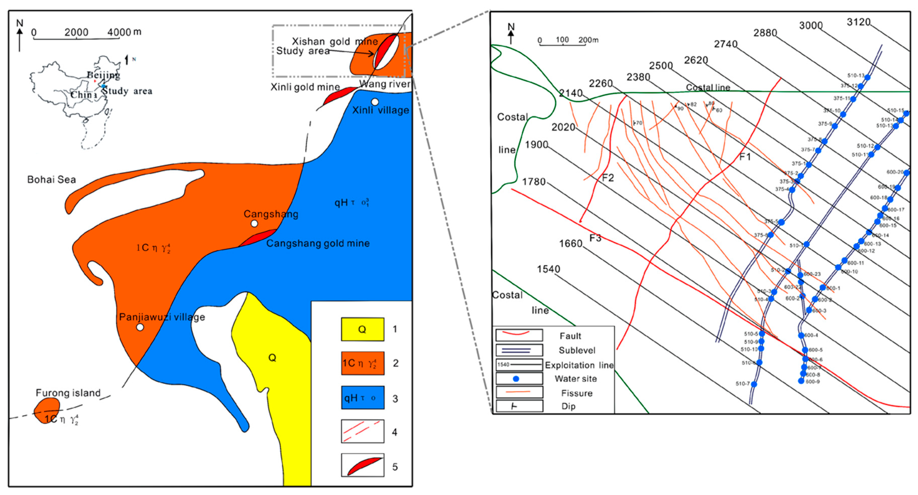
2. Study Area
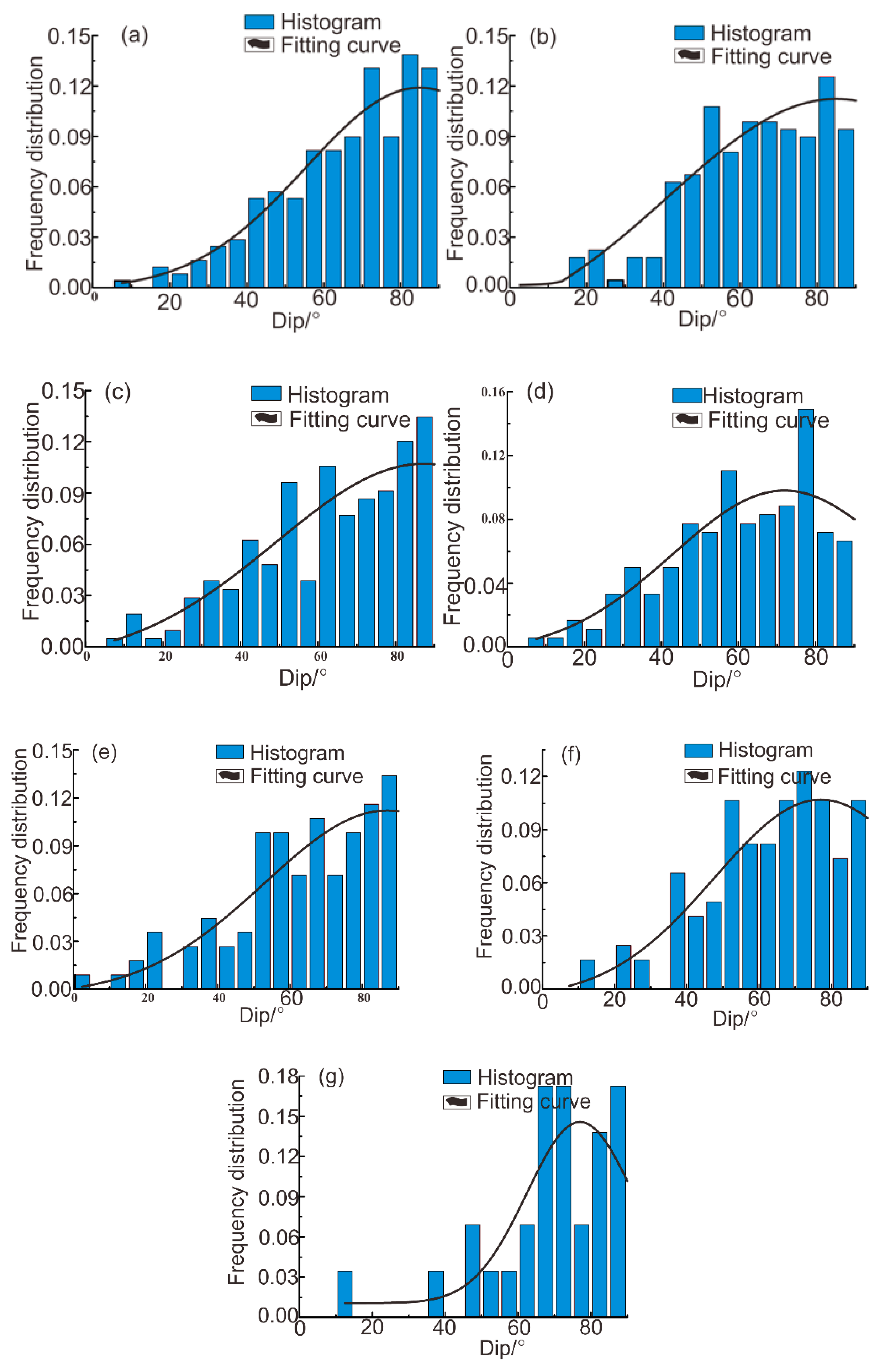
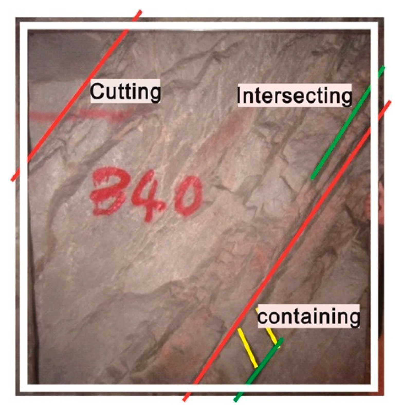
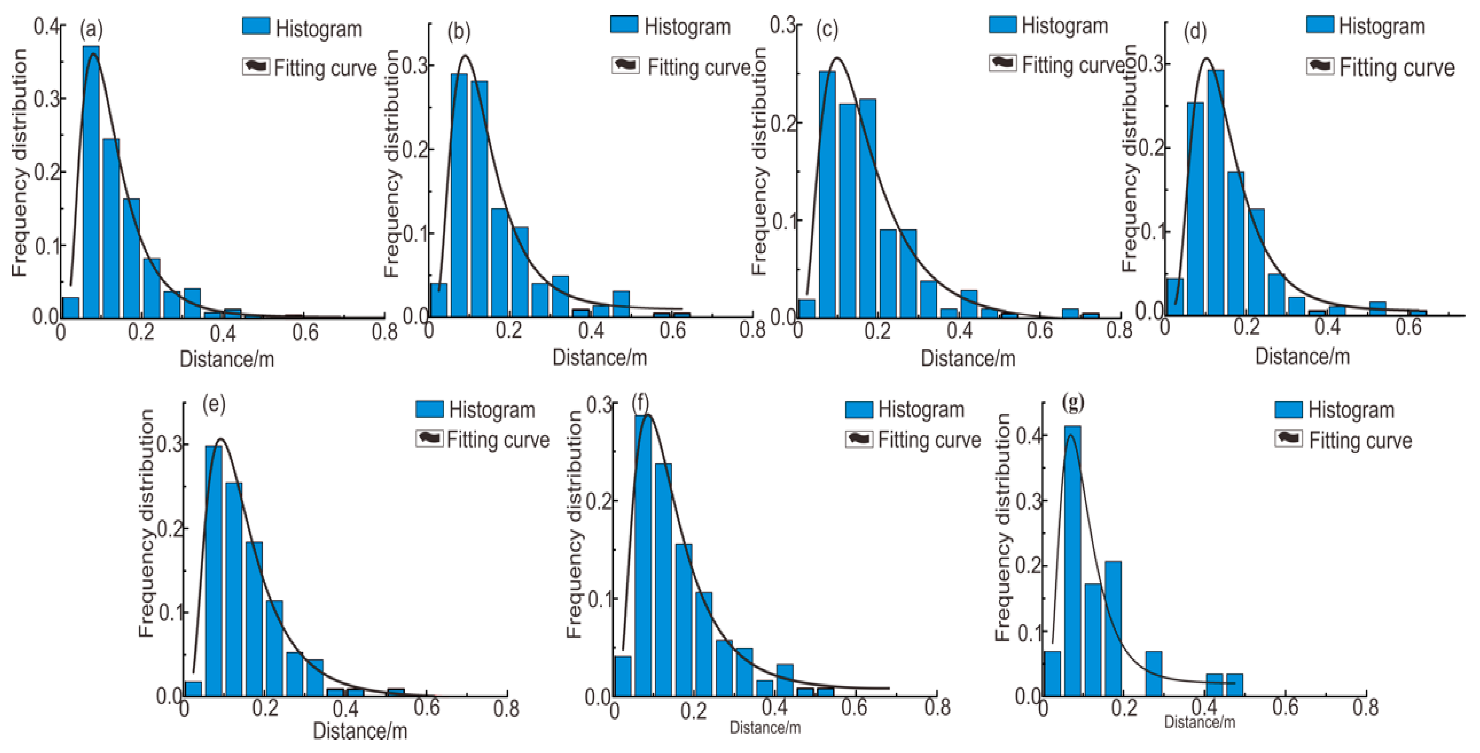
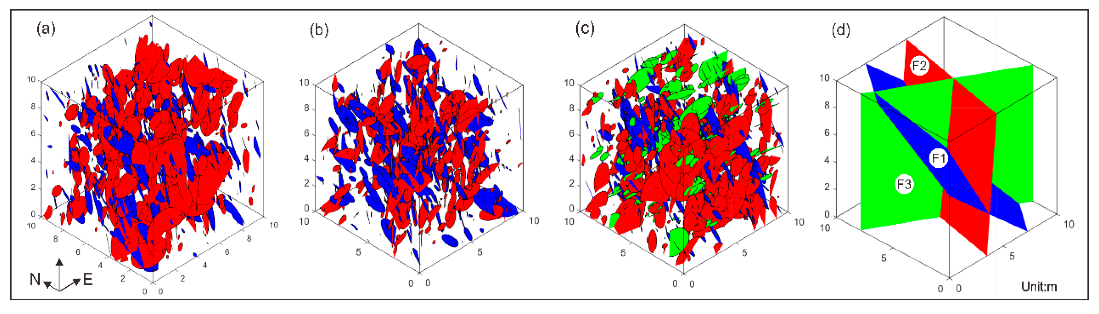
2.1. Geological Structures
2.2. Hydrogeology
3. Methods
3.1. Water Sampling
3.2. Principal Component Analysis (PCA)
3.3. Hierarchical Cluster Analysis (HCA)
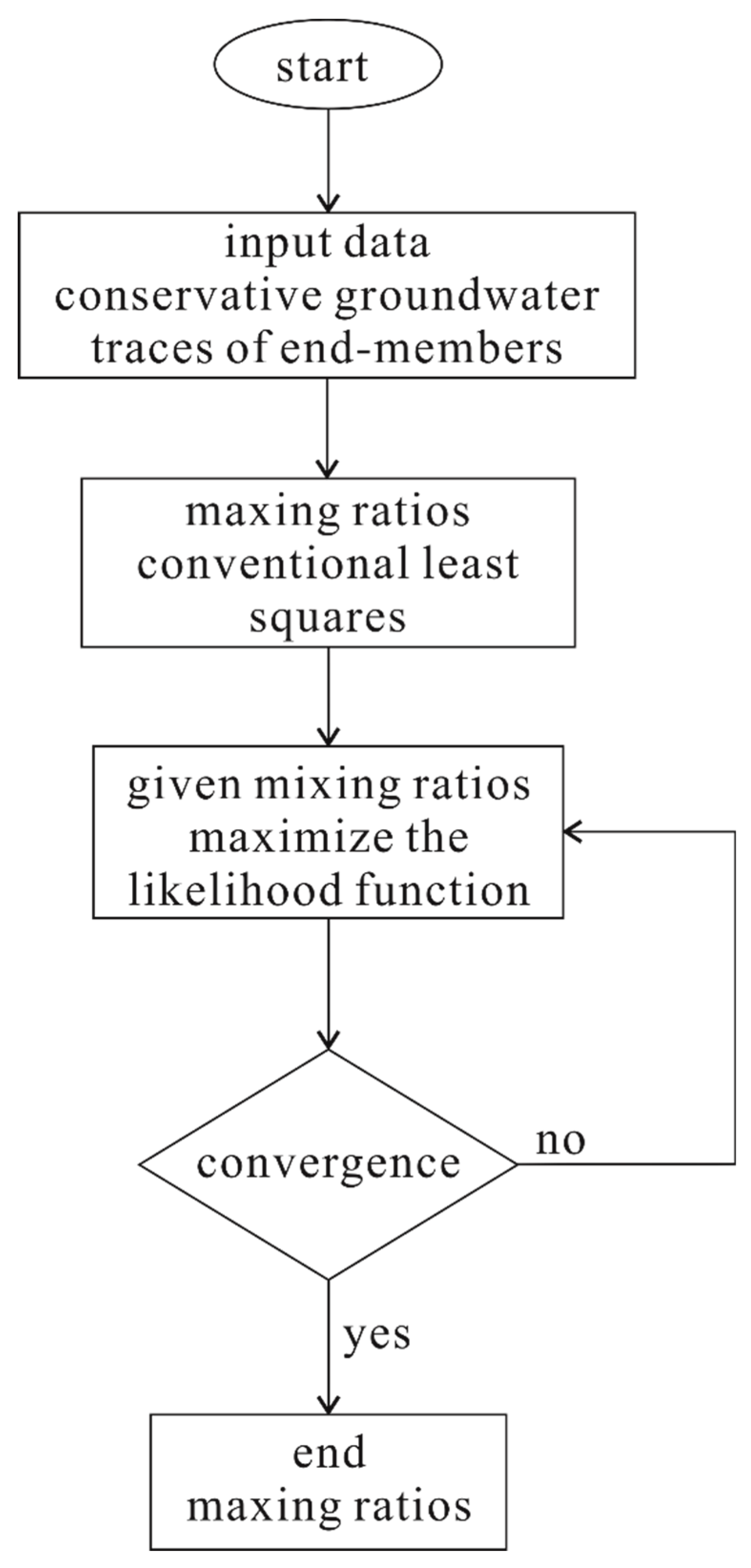
3.4. End-Member Mixing Analysis (EMMA)
4. Application and Results
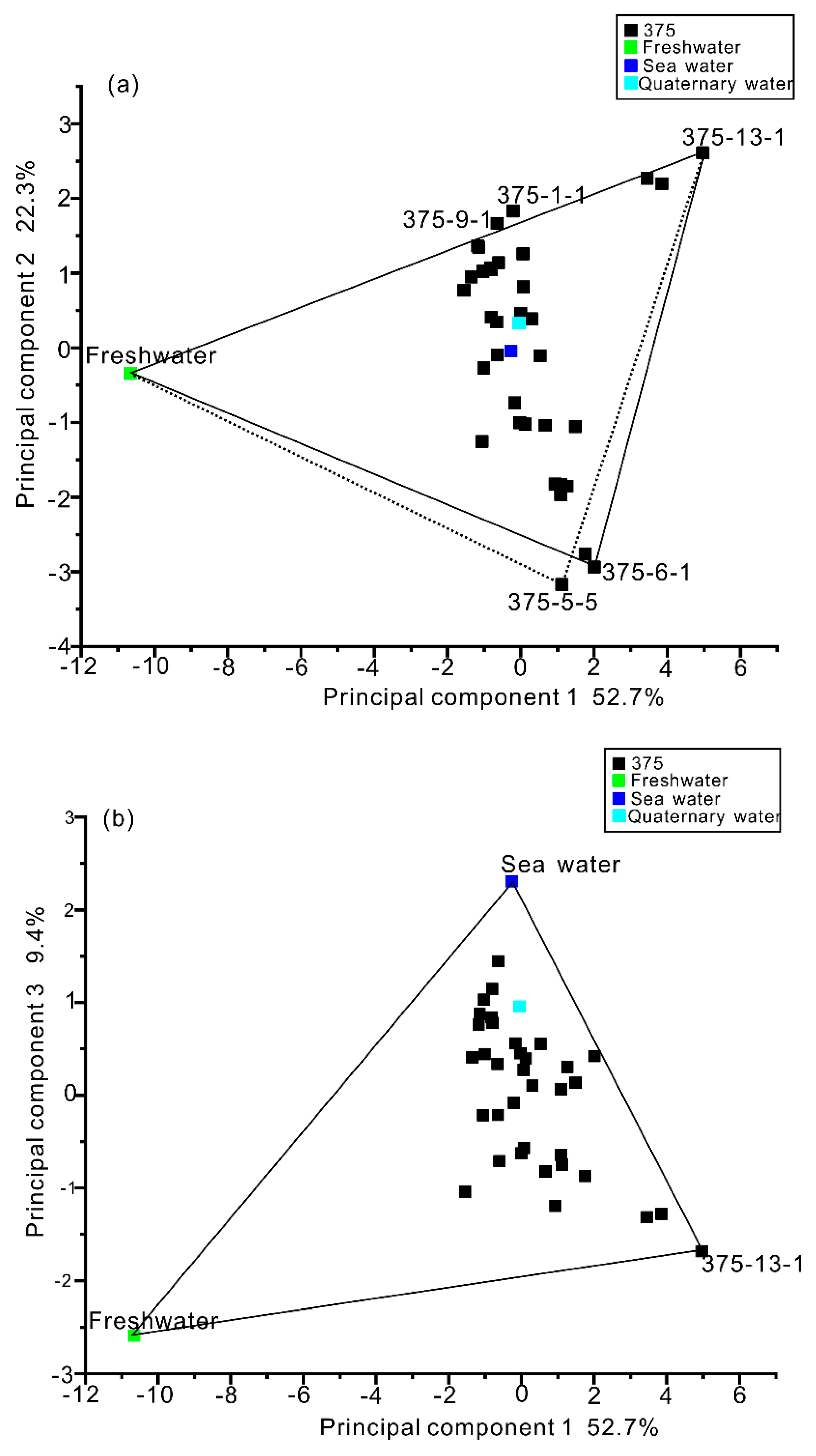
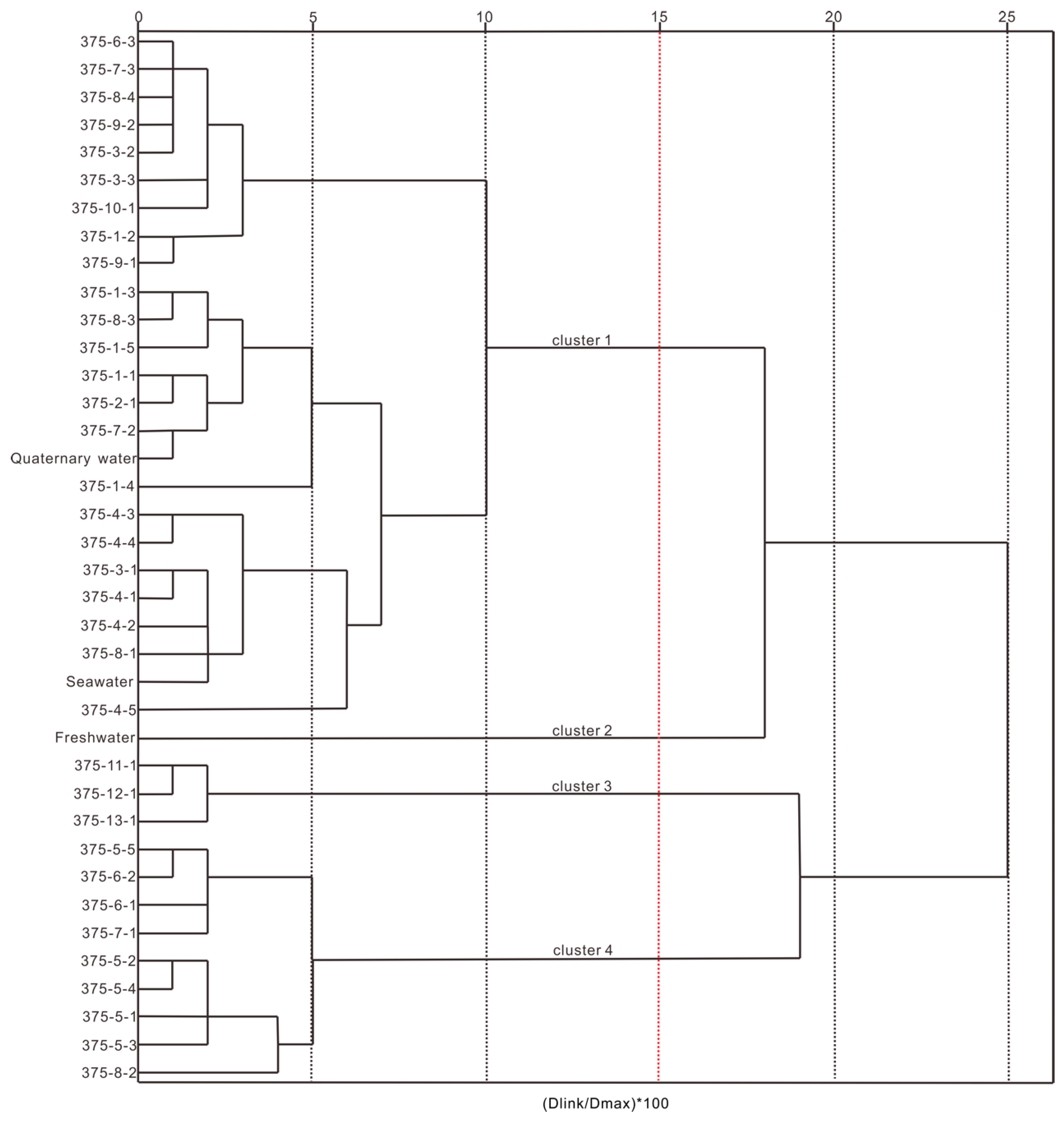
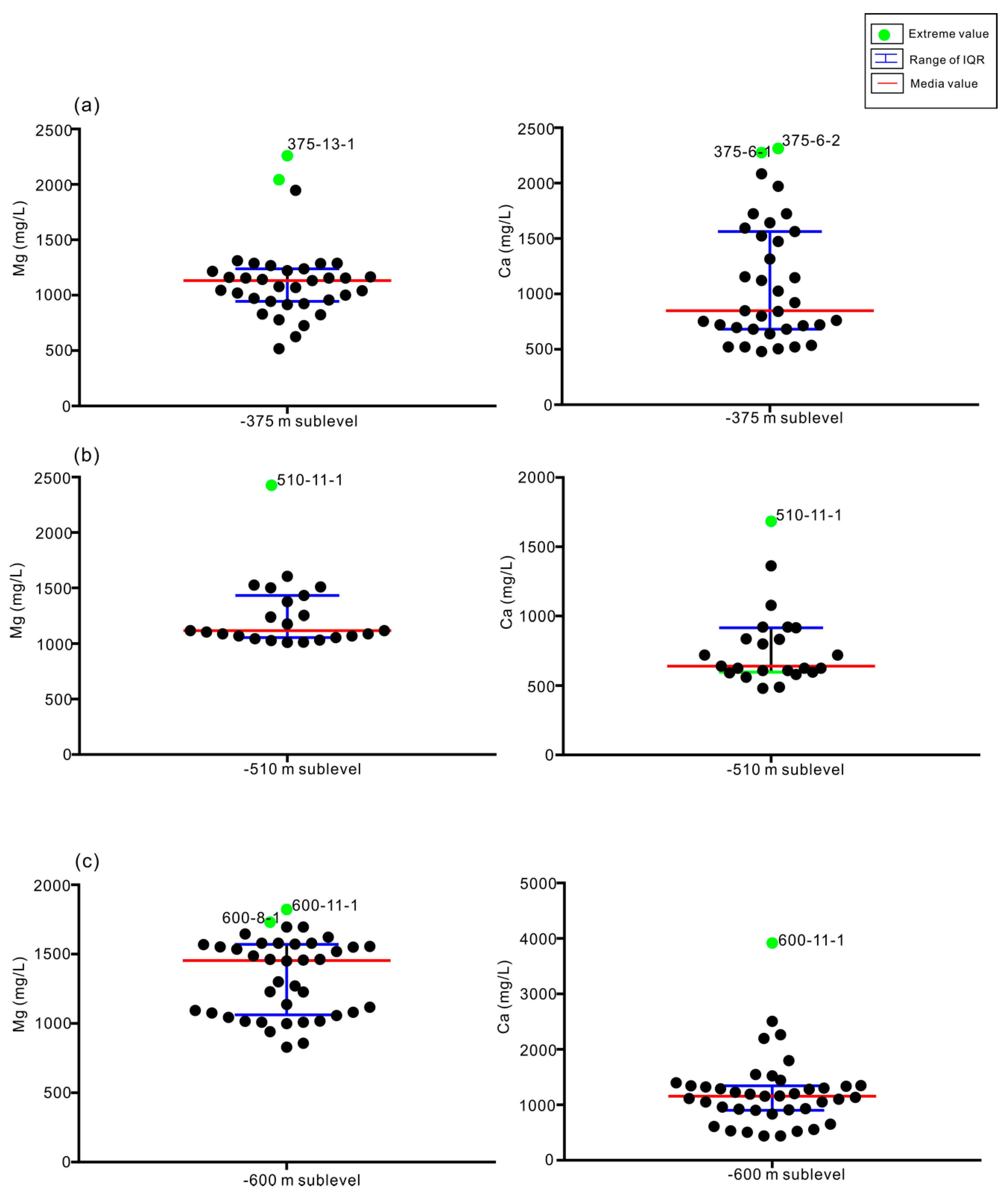
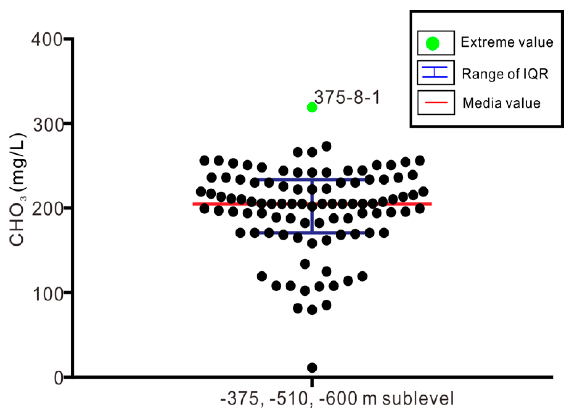
4.1. Scenario 1: −375-m Sublevel
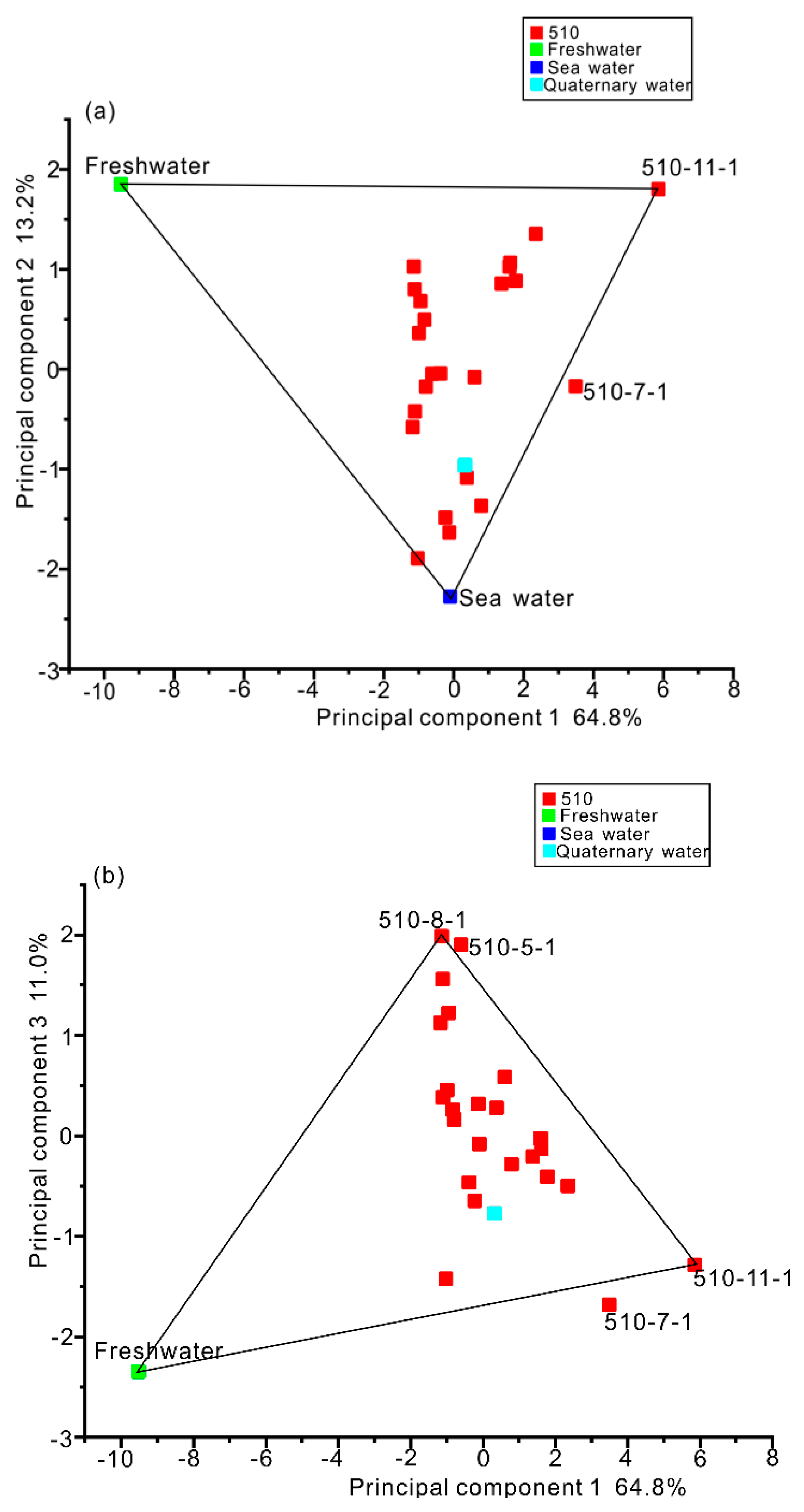
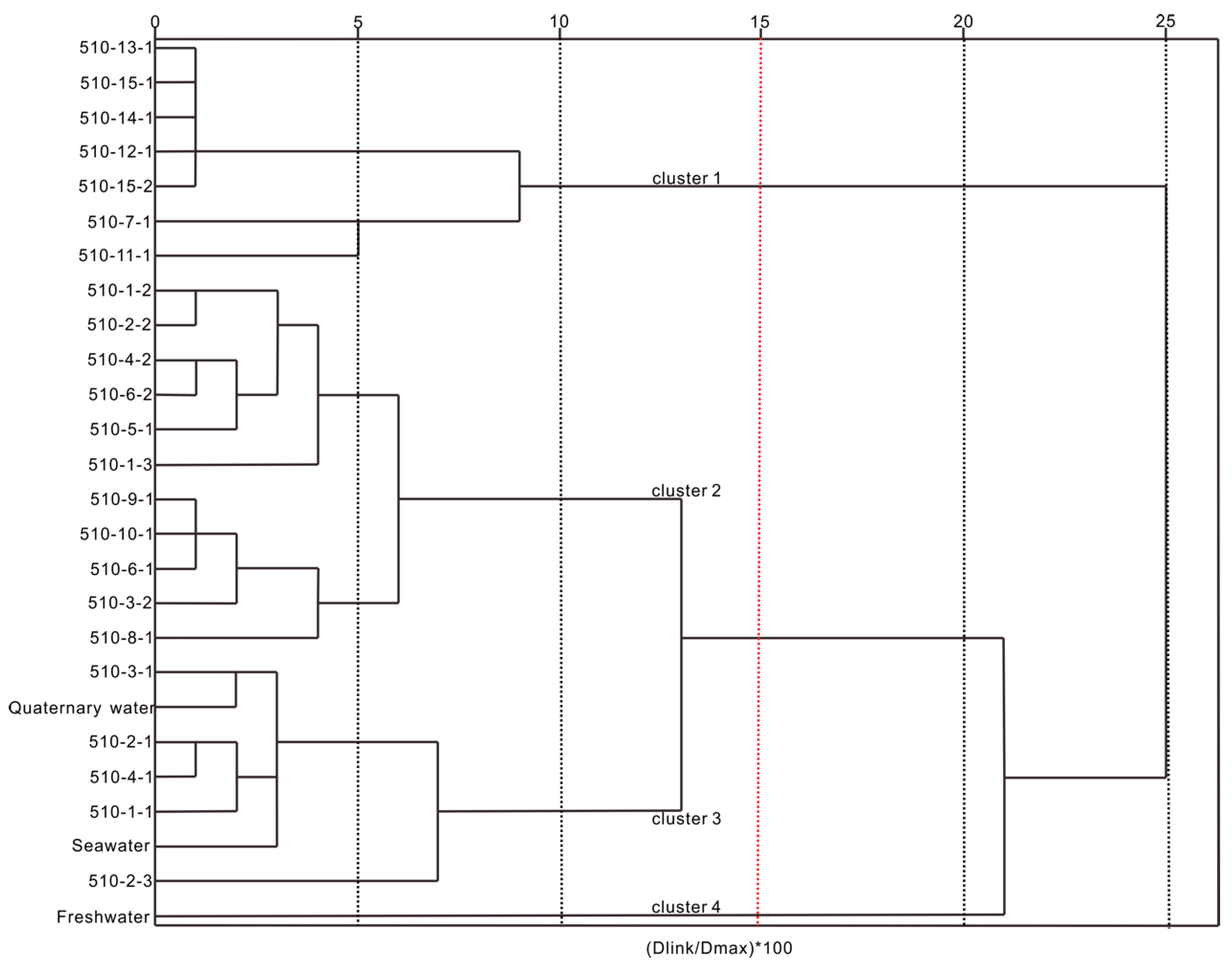
4.2. Scenario 2: The −510-m Sublevel
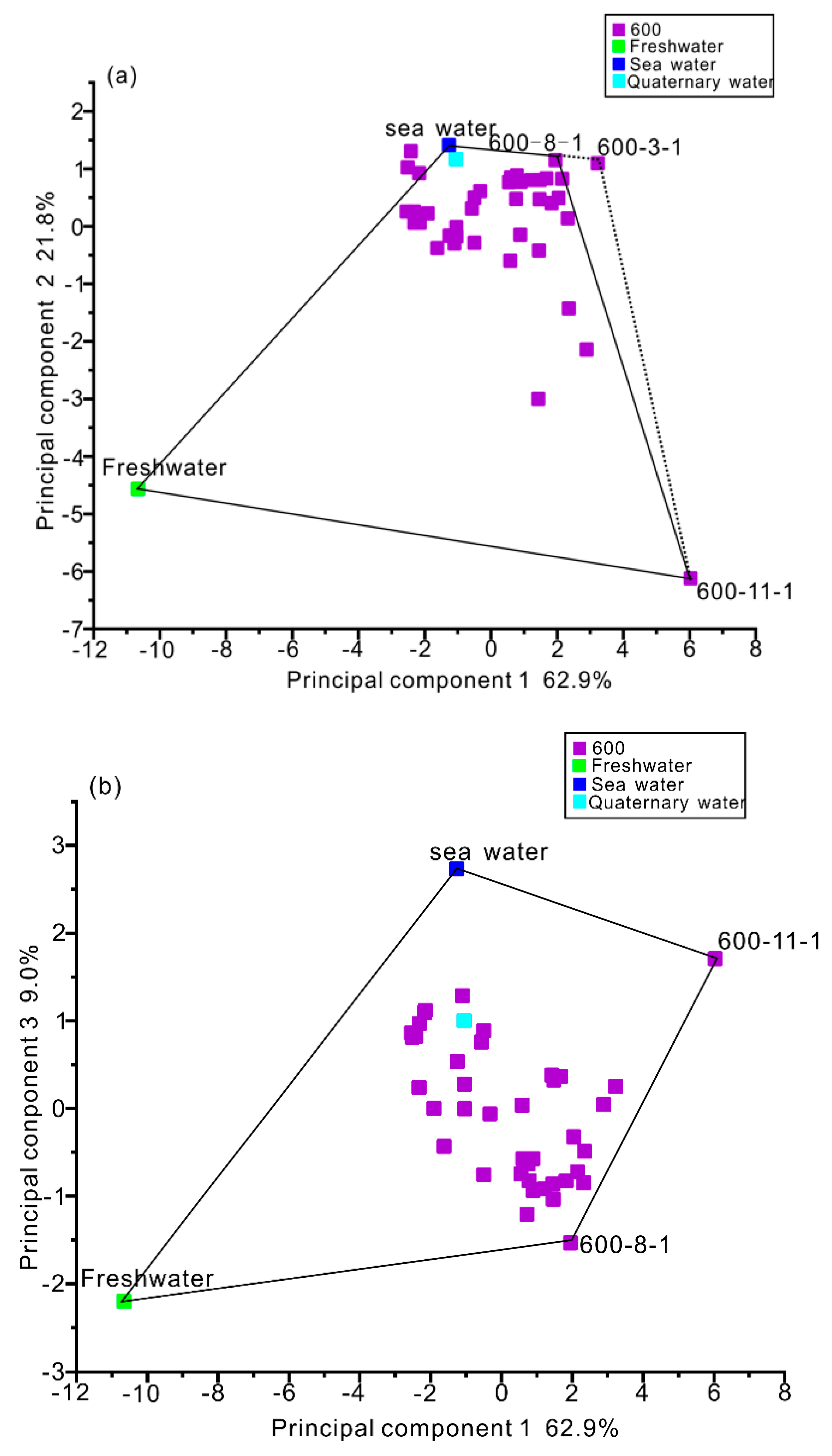
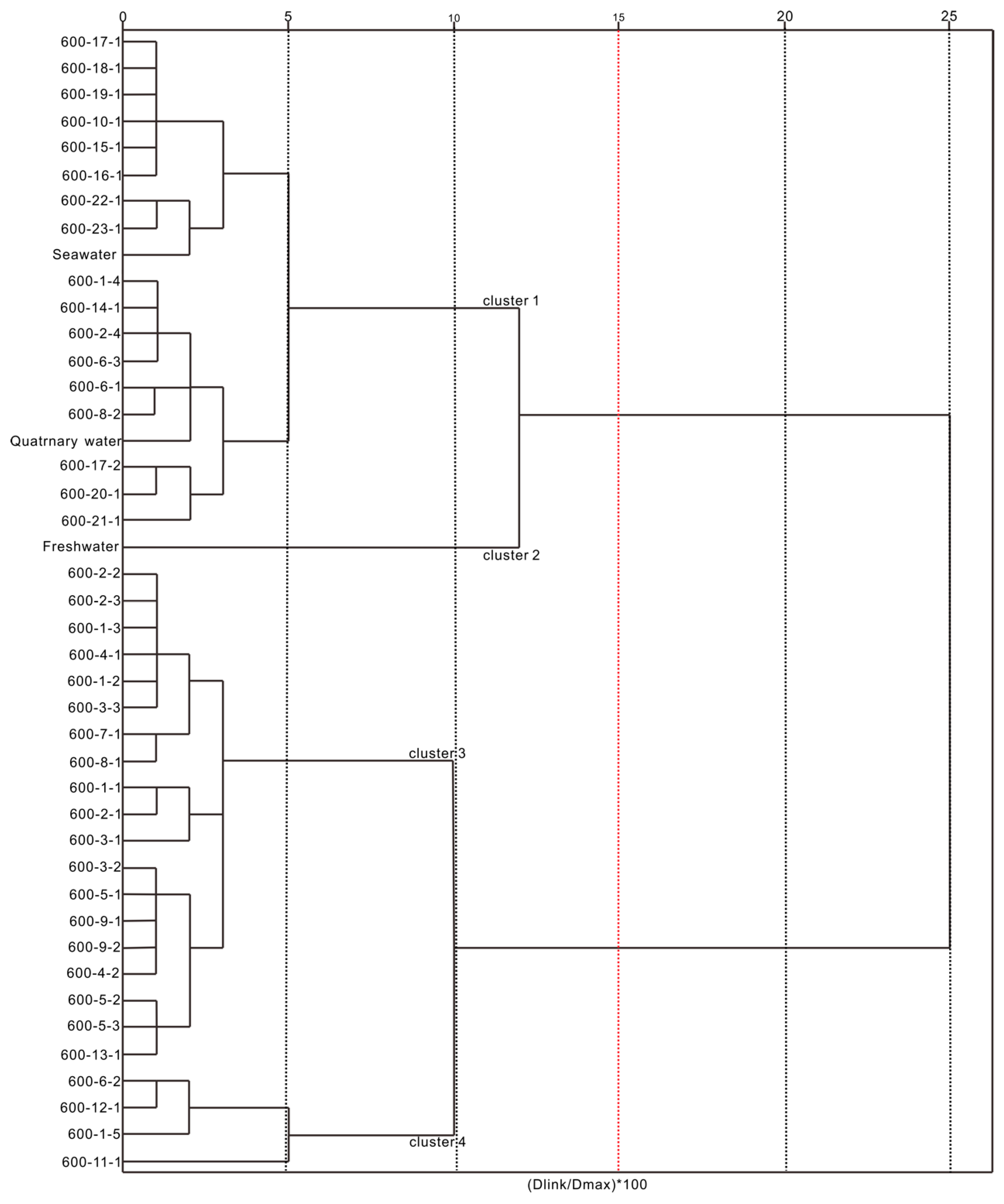
4.3. Scenario 3: −600-m Sublevel
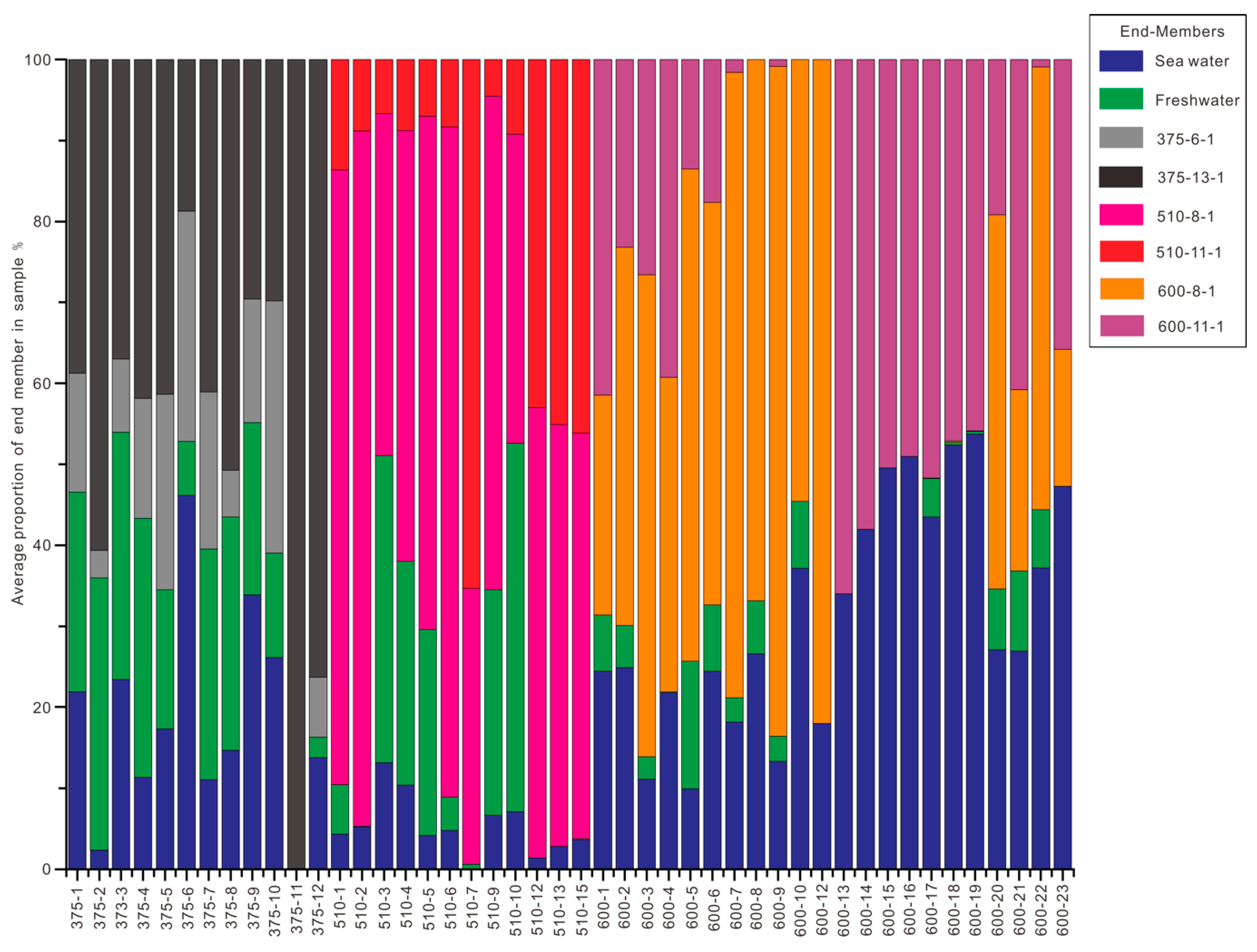
4.4. Mixing Ratios of Water Sources
5. Discussion
5.1. Choice of End-Members in the PCA and HCA Models
5.2. Choice of Conservative Groundwater Tracers in the EMMA Model
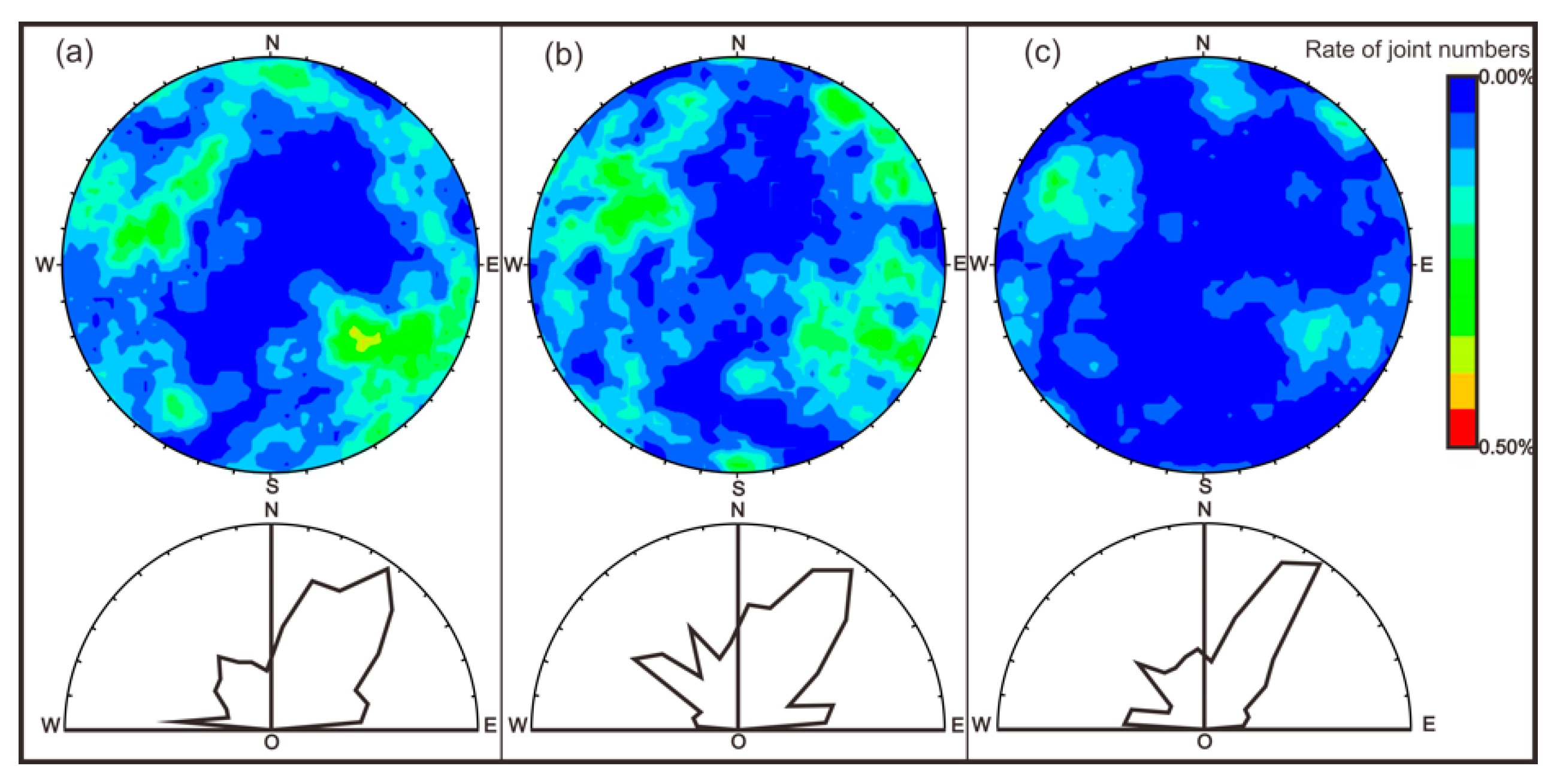
5.3. Three-Dimensional Geological Model
6. Conclusions
Supplementary Materials
Author Contributions
Funding
Conflicts of Interest
References
- Carrera, J.; Vázquez-Suñé, E.; Castillo, O.; Sánchez-Vila, X. A methodology to compute mixing ratios with uncertain end-members. Water Resour. Res. 2004, 40, 12. [Google Scholar] [CrossRef]
- Rasmussen, J. Estimating terrestrial contribution to stream invertebrates and periphyton using a gradient-based mixing model for δ13C. J. Anim. Ecol. 2010, 79, 393–402. [Google Scholar] [CrossRef] [PubMed]
- IJmker, J.; Stauch, G.; Dietze, E.; Hartmann, K.; Diekmann, B.; Lockot, G.; Opitz, S.; Wünnemann, B.; Lehmkuhl, F. Characterisation of transport processes and sedimentary deposits by statistical end-member mixing analysis of terrestrial sediments in the Donggi Cona lake catchment, NE Tibetan Plateau. Sediment. Geol. 2012, 281, 166–179. [Google Scholar] [CrossRef]
- Keay, S.; Collins, W.; McCulloch, M. A three-component Sr-Nd isotopic mixing model for granitoid genesis, Lachlan fold belt, eastern Australia. Geology 1997, 25, 307–310. [Google Scholar] [CrossRef]
- Weltje, G.J. End-member modeling of compositional data: Numerical-statistical algorithms for solving the explicit mixing problem. Math. Geol. 1997, 29, 503–549. [Google Scholar] [CrossRef]
- Huntoon, P.W. Fault Controlled Ground-Water Circulation Under the Colorado River, Marble Canyon, Arizona. Groundwater 1981, 19, 20–27. [Google Scholar] [CrossRef]
- Hooper, R.P.; Christophersen, N.; Peters, N.E. Modelling streamwater chemistry as a mixture of soilwater end-members—An application to the Panola Mountain catchment, Georgia, USA. J. Hydrol. 1990, 116, 321–343. [Google Scholar] [CrossRef]
- Christophersen, N.; Hooper, R.P. Multivariate analysis of stream water chemical data: The use of principal components analysis for the end-member mixing problem. Water Resour. Res. 1992, 28, 99–107. [Google Scholar] [CrossRef]
- Doctor, D.H.; Alexander, E.C.; Petrič, M.; Kogovšek, J.; Urbanc, J.; Lojen, S.; Stichler, W. Quantification of karst aquifer discharge components during storm events through end-member mixing analysis using natural chemistry and stable isotopes as tracers. Hydrogeol. J. 2006, 14, 1171–1191. [Google Scholar] [CrossRef]
- Laaksoharju, M.; Skårman, C.; Skårman, E. Multivariate mixing and mass balance (M3) calculations, a new tool for decoding hydrogeochemical information. Appl. Geochem. 1999, 14, 861–871. [Google Scholar] [CrossRef]
- Acharya, A.; Piechota, T.C.; Stephen, H.; Tootle, G. Modeled streamflow response under cloud seeding in the North Platte River watershed. J. Hydrol. 2011, 409, 305–314. [Google Scholar] [CrossRef]
- Valder, J.F.; Long, A.J.; Davis, A.D.; Kenner, S.J. Multivariate statistical approach to estimate mixing proportions for unknown end members. J. Hydrol. 2012, 460, 65–76. [Google Scholar] [CrossRef]
- Gorgoglione, A.; Gioia, A.; Iacobellis, V. A framework for assessing modeling performance and effects of rainfall-catchment-drainage characteristics on nutrient urban runoff in poorly gauged watersheds. Sustainability 2019, 11, 4933. [Google Scholar] [CrossRef]
- Ouarda, T.B.; Charron, C.; Hundecha, Y.; St-Hilaire, A.; Chebana, F. Introduction of the GAM model for regional low-flow frequency analysis at ungauged basins and comparison with commonly used approaches. Environ. Model. Softw. 2018, 109, 256–271. [Google Scholar] [CrossRef]
- Wu, B.; Wang, G.; Wang, Z.; Liu, C.; Ma, J. Integrated hydrologic and hydrodynamic modeling to assess water exchange in a data-scarce reservoir. J. Hydrol. 2017, 555, 15–30. [Google Scholar] [CrossRef]
- Davis, J.C.; Sampson, R.J. Statistics and Data Analysis in Geology; Wiley: New York, USA, 1986; Volume 646. [Google Scholar]
- Moore, P.J.; Martin, J.B.; Screaton, E.J. Geochemical and statistical evidence of recharge, mixing, and controls on spring discharge in an eogenetic karst aquifer. J. Hydrol. 2009, 376, 443–455. [Google Scholar] [CrossRef]
- Liu, G.; Ma, F.; Liu, G.; Zhao, H.; Guo, J.; Cao, J. Application of Multivariate Statistical Analysis to Identify Water Sources in A Coastal Gold Mine, Shandong, China. Sustainability 2019, 11, 3345. [Google Scholar] [CrossRef]
- Colby, N. The use of 2-way cluster analysis as a tool for delineating trends in hydrogeologic units and development of a conceptual model. In Proceedings of the International Ground Water Modeling Center (IGWMC) 1993 Ground Water Modeling Conference, Golden, CO, USA, 9–12 June 1993; IGWMC: Golden, CO, USA; pp. 91–100. [Google Scholar]
- Woocay, A.; Walton, J. Multivariate analyses of water chemistry: Surface and ground water interactions. Groundwater 2008, 46, 437–449. [Google Scholar] [CrossRef]
- Suk, H.; Lee, K.K. Characterization of a ground water hydrochemical system through multivariate analysis: Clustering into ground water zones. Groundwater 1999, 37, 358–366. [Google Scholar] [CrossRef]
- Mishra, S.; Kumar, A.; Yadav, S.; Singhal, M. Assessment of heavy metal contamination in water of Kali River using principle component and cluster analysis, India. Sustain. Water Resour. Manag. 2018, 4, 573–581. [Google Scholar] [CrossRef]
- Mazurek, R.; Kowalska, J.; Gąsiorek, M.; Zadrożny, P.; Józefowska, A.; Zaleski, T.; Kępka, W.; Tymczuk, M.; Orłowska, K. Assessment of heavy metals contamination in surface layers of Roztocze National Park forest soils (SE Poland) by indices of pollution. Chemosphere 2017, 168, 839–850. [Google Scholar] [CrossRef] [PubMed]
- Praus, P. Principal Component Weighted Index for Wastewater Quality Monitoring. Water 2019, 11, 2376. [Google Scholar] [CrossRef]
- Che, H.; Zhang, J. Water Mass Analysis and End-Member Mixing Contribution Using Coupled Radiogenic Nd Isotopes and Nd Concentrations: Interaction Between Marginal Seas and the Northwestern Pacific. Geophys. Res. Lett. 2018, 45, 2388–2395. [Google Scholar] [CrossRef]
- Pelizardi, F.; Bea, S.A.; Carrera, J.; Vives, L. Identifying geochemical processes using End Member Mixing Analysis to decouple chemical components for mixing ratio calculations. J. Hydrol. 2017, 550, 144–156. [Google Scholar] [CrossRef]
- Williams, M.R.; Leydecker, A.; Brown, A.D.; Melack, J.M. Processes regulating the solute concentrations of snowmelt runoff in two subalpine catchments of the Sierra Nevada, California. Water Resour. Res. 2001, 37, 1993–2008. [Google Scholar] [CrossRef]
- Qian, J.; Wang, L.; Ma, L.; Lu, Y.; Zhao, W.; Zhang, Y. Multivariate statistical analysis of water chemistry in evaluating groundwater geochemical evolution and aquifer connectivity near a large coal mine, Anhui, China. Environ. Earth Sci. 2016, 75, 747. [Google Scholar] [CrossRef]
- Wang, Y.; Wang, P.; Bai, Y.; Tian, Z.; Li, J.; Shao, X.; Mustavich, L.F.; Li, B.-L. Assessment of surface water quality via multivariate statistical techniques: A case study of the Songhua River Harbin region, China. J. Hydro-Environ. Res 2013, 7, 30–40. [Google Scholar] [CrossRef]
- Wu, S.; Yu, Z.; Zou, D.; Zhang, H. Structural features and Cenozoic evolution of the Tan-Lu fault zone in the Laizhou Bay, Bohai Sea. Marine Geol. Quat. Geol. 2006, 26, 101. [Google Scholar]
- Luo, J.; Pang, Z.; Kong, Y.; Wang, Y. Geothermal potential evaluation and development prioritization based on geochemistry of geothermal waters from Kangding area, western Sichuan, China. Environ. Earth Sci. 2017, 76, 343. [Google Scholar] [CrossRef]
- Craig, H. Standard for reporting concentrations of deuterium and oxygen-18 in natural waters. Science 1961, 133, 1833–1834. [Google Scholar] [CrossRef]
- Shrestha, S.; Kazama, F. Assessment of surface water quality using multivariate statistical techniques: A case study of the Fuji river basin, Japan. Environ. Model. Softw. 2007, 22, 464–475. [Google Scholar] [CrossRef]
- Cortes, J.; Muñoz, L.; Gonzalez, C.; Niño, J.; Polo, A.; Suspes, A.; Siachoque, S.; Hernández, A.; Trujillo, H. Hydrogeochemistry of the formation waters in the San Francisco field, UMV basin, Colombia–A multivariate statistical approach. J. Hydrol. 2016, 539, 113–124. [Google Scholar] [CrossRef]
- Otto, M. Multivariate methods. In Analytical Chemistry; Keller, R., Mermet, J.M., Otto, M., Eds.; Widmer, H.M. Wiley-VCH: Weinheim, Germany, 1998. [Google Scholar]
- Raiber, M.; White, P.A.; Daughney, C.J.; Tschritter, C.; Davidson, P.; Bainbridge, S.E. Three-dimensional geological modelling and multivariate statistical analysis of water chemistry data to analyse and visualise aquifer structure and groundwater composition in the Wairau Plain, Marlborough District, New Zealand. J. Hydrol. 2012, 436, 13–34. [Google Scholar] [CrossRef]
- Gu, H.; Ma, F.; Guo, J.; Li, K.; Lu, R. Assessment of water sources and mixing of groundwater in a coastal mine: The Sanshandao gold mine, China. Mine Water Environ. 2018, 37, 351–365. [Google Scholar] [CrossRef]
- Gu, H.; Ma, F.; Guo, J.; Zhao, H.; Lu, R.; Liu, G. A spatial mixing model to assess groundwater dynamics affected by mining in a coastal fractured aquifer, China. Mine Water Environ. 2018, 37, 405–420. [Google Scholar] [CrossRef]
- Wu, F. Principles of Statistical Mechanics of Rock Masses; China University of Geosciences Press: Wuhan, China, 1993. [Google Scholar]
- Li, Q. Estimation of Trace Length and Connectivity Rate of Joint Based on Digital Close-Range Photogrammetry; Jilin University: Jilin, China, 2017. [Google Scholar]


| Location | End-Members of −375m Sublevel | |||
|---|---|---|---|---|
| Freshwater | Seawater | 375-6-1 | 375-13-1 | |
| 375-1-1 | 0.315 | 0.092 | 0 | 0.593 |
| 375-1-2 | 0.06 | 0.542 | 0.361 | 0.037 |
| 375-1-3 | 0.122 | 0.392 | 0.325 | 0.162 |
| 375-1-4 | 0.366 | 0.023 | 0 | 0.611 |
| 375-1-5 | 0.37 | 0.045 | 0.05 | 0.535 |
| 375-2-1 | 0.336 | 0.024 | 0.034 | 0.607 |
| 375-3-1 | 0.027 | 0.702 | 0.271 | 0 |
| 375-3-2 | 0.459 | 0 | 0.001 | 0.54 |
| 375-3-3 | 0.431 | 0 | 0 | 0.569 |
| 375-4-1 | 0.318 | 0.102 | 0.239 | 0.34 |
| 375-4-2 | 0.442 | 0 | 0.026 | 0.532 |
| 375-4-3 | 0.113 | 0.371 | 0.423 | 0.092 |
| 375-4-4 | 0.362 | 0.058 | 0.02 | 0.56 |
| 375-4-5 | 0.363 | 0.036 | 0.033 | 0.568 |
| 375-5-1 | 0.161 | 0.162 | 0.19 | 0.487 |
| 375-5-2 | 0.11 | 0.281 | 0.318 | 0.291 |
| 375-5-3 | 0.222 | 0.107 | 0.322 | 0.349 |
| 375-5-4 | 0.306 | 0.005 | 0.002 | 0.687 |
| 375-5-5 | 0.061 | 0.311 | 0.374 | 0.253 |
| 375-6-2 | 0.037 | 0.308 | 0.35 | 0.305 |
| 375-6-3 | 0.096 | 0.615 | 0.22 | 0.069 |
| 375-7-1 | 0.105 | 0.213 | 0.391 | 0.291 |
| 375-7-2 | 0.399 | 0.035 | 0.053 | 0.513 |
| 375-7-3 | 0.35 | 0.085 | 0.137 | 0.429 |
| 375-8-1 | 0.364 | 0 | 0.076 | 0.56 |
| 375-8-2 | 0.203 | 0.17 | 0.047 | 0.58 |
| 375-8-3 | 0.191 | 0.322 | 0.107 | 0.38 |
| 375-8-4 | 0.393 | 0.097 | 0 | 0.51 |
| 375-9-1 | 0.337 | 0.059 | 0.084 | 0.52 |
| 375-9-2 | 0.089 | 0.619 | 0.221 | 0.072 |
| 375-10-1 | 0.129 | 0.261 | 0.311 | 0.298 |
| 375-11-1 | 0 | 0 | 0 | 1 |
| 375-12-1 | 0.025 | 0.138 | 0.074 | 0.763 |
| Quaternary water | 0.406 | 0.025 | 0.004 | 0.565 |
| Location | End-Members of −510 m Sublevel | |||
|---|---|---|---|---|
| Freshwater | Seawater | 510-8-1 | 510-11-1 | |
| 510-1-1 | 0.178 | 0.029 | 0.595 | 0.197 |
| 510-1-2 | 0 | 0.057 | 0.88 | 0.063 |
| 510-1-3 | 0.005 | 0.045 | 0.8 | 0.149 |
| 510-2-1 | 0.002 | 0.049 | 0.803 | 0.416 |
| 510-2-2 | 0 | 0.077 | 0.839 | 0.084 |
| 510-2-3 | 0 | 0.031 | 0.935 | 0.034 |
| 510-3-1 | 0.749 | 0.234 | 0.017 | 0 |
| 510-3-2 | 0.008 | 0.03 | 0.829 | 0.133 |
| 510-4-1 | 0.245 | 0.056 | 0.535 | 0.164 |
| 510-4-2 | 0 | 0.067 | 0.859 | 0.074 |
| 510-5-1 | 0.254 | 0.042 | 0.634 | 0.07 |
| 510-6-1 | 0.083 | 0.033 | 0.824 | 0.061 |
| 510-6-2 | 0 | 0.063 | 0.832 | 0.105 |
| 510-7-1 | 0.006 | 0 | 0.341 | 0.653 |
| 510-9-1 | 0.278 | 0.067 | 0.61 | 0.045 |
| 510-10-1 | 0.455 | 0.071 | 0.382 | 0.092 |
| 510-12-1 | 0.001 | 0.013 | 0.556 | 0.43 |
| 510-13-1 | 0 | 0.028 | 0.521 | 0.451 |
| 510-15-1 | 0.001 | 0.037 | 0.5 | 0.461 |
| Quaternary water | 0.401 | 0.061 | 0.368 | 0.17 |
| Location | End-Members of −600 m Sublevel | |||
|---|---|---|---|---|
| Freshwater | Seawater | 600-8-1 | 600-11-1 | |
| 600-1-1 | 0.117 | 0.063 | 0.821 | 0 |
| 600-1-2 | 0 | 0.312 | 0 | 0.688 |
| 600-1-3 | 0 | 0.32 | 0 | 0.68 |
| 600-1-4 | 0.229 | 0.232 | 0.539 | 0 |
| 600-1-5 | 0 | 0.296 | 0 | 0.704 |
| 600-2-1 | 0.094 | 0.112 | 0.782 | 0.013 |
| 600-2-2 | 0 | 0.337 | 0.002 | 0.661 |
| 600-2-3 | 0.001 | 0.232 | 0.514 | 0.253 |
| 600-2-4 | 0.112 | 0.315 | 0.573 | 0 |
| 600-3-1 | 0.053 | 0 | 0.946 | 0 |
| 600-3-2 | 0 | 0.203 | 0 | 0.797 |
| 600-3-3 | 0.03 | 0.132 | 0.838 | 0 |
| 600-4-1 | 0.002 | 0.317 | 0 | 0.68 |
| 600-4-2 | 0 | 0.119 | 0.777 | 0.105 |
| 600-5-1 | 0 | 0.132 | 0.462 | 0.406 |
| 600-5-2 | 0.086 | 0.167 0 | 0.748 | 0 |
| 600-5-3 | 0.385 | 0.615 | 0 | |
| 600-6-1 | 0.037 | 0.262 | 0.701 | 0 |
| 600-6-2 | 0.208 | 0.002 | 0.79 | 0 |
| 600-6-3 | 0 | 0.469 | 0 | 0.53 |
| 600-7-1 | 0.03 | 0.182 | 0.773 | 0.016 |
| 600-8-2 | 0.066 | 0.266 | 0.669 | 0 |
| 600-9-1 | 0.026 | 0.116 | 0.84 | 0.017 |
| 600-9-2 | 0.035 | 0.151 | 0.814 | 0 |
| 600-10-1 | 0.083 | 0.371 | 0.545 | 0 |
| 600-12-1 | 0 | 0.18 | 0 | 0.82 |
| 600-13-1 | 0 | 0.34 | 0 | 0.66 |
| 600-14-1 | 0 | 0.419 | 0 | 0.58 |
| 600-15-1 | 0 | 0.495 | 0 | 0.504 |
| 600-16-1 | 0 | 0.509 | 0 | 0.49 |
| 600-17-1 | 0 | 0.52 | 0 | 0.48 |
| 600-17-2 | 0.095 | 0.35 | 0.001 | 0.554 |
| 600-18-1 | 0.003 | 0.524 | 0.002 | 0.471 |
| 600-19-1 | 0.003 | 0.537 | 0.001 | 0.458 |
| 600-20-1 | 0.075 | 0.271 | 0.462 | 0.192 |
| 600-21-1 | 0.099 | 0.269 | 0.224 | 0.408 |
| 600-22-1 | 0.072 | 0.372 | 0.547 | 0.009 |
| 600-23-1 | 0 | 0.473 | 0.169 | 0.358 |
| Quaternary water | 0.186 | 0.287 | 0.527 | 0 |
| −375-m Sublevel | −510-m Sublevel | −600-m Sublevel | |||||||
|---|---|---|---|---|---|---|---|---|---|
| PC1 | PC2 | PC3 | PC1 | PC2 | PC3 | PC1 | PC2 | PC3 | |
| K+ | 0.403 | −0.308 | 0.837 | 0.370 | −0.807 | 0.377 | 0.134 | 0.498 | 0.851 |
| Na+ | 0.986 | 0.029 | −0.043 | 0.987 | 0.058 | 0.057 | 0.966 | 0.200 | −0.055 |
| Ca2+ | 0.630 | −0.580 | −0.381 | 0.855 | 0.328 | −0.250 | 0.768 | −0.596 | 0.020 |
| Mg2+ | 0.630 | 0.735 | −0.057 | 0.962 | 0.160 | −0.017 | 0.894 | 0.260 | −0.208 |
| a Cl− | 0.978 | 0.088 | −0.115 | 0.967 | 0.147 | −0.006 | 0.990 | 0.023 | −0.056 |
| SO42+ | 0.830 | 0.110 | 0.112 | 0.942 | −0.104 | 0.165 | 0.705 | 0.660 | −0.053 |
| HCO3− | −0.128 | 0.932 | −0.013 | 0.047 | 0.600 | 0.530 | −0.459 | 0.724 | −0.334 |
| pH | −0.166 | 0.605 | 0.166 | −0.297 | 0.155 | 0.757 | −0.583 | 0.695 | −0.104 |
| EC | 0.822 | −0.029 | 0.153 | 0.904 | −0.332 | 0.095 | 0.967 | 0.156 | 0.032 |
| TDS | 0.987 | 0.065 | −0.100 | 0.994 | 0.081 | −0.002 | 0.993 | 0.065 | −0.044 |
| Eigenvalue | 5.269 | 2.231 | 0.937 | 6.483 | 1.320 | 1.098 | 6.288 | 2.181 | 0.902 |
| PEVCPEV | 52.7 | 22.3 | 9.4 | 64.830 | 13.198 | 10.978 | 62.878 | 21.811 | 9.02 |
| 52.7 | 75.0 | 84.4 | 64.830 | 78.028 | 89.006 | 62.878 | 84.689 | 93.710 | |
| −375-m Sublevel | ||||||||||
|---|---|---|---|---|---|---|---|---|---|---|
| K+ | Na+ | Ca2+ | Mg2+ | Cl− | SO42+ | HCO3− | pH | EC | TDSes | |
| K+ | 1.000 | |||||||||
| Na+ | 0.359 | 1.000 | ||||||||
| Ca2+ | 0.141 | 0.605 | 1.000 | |||||||
| Mg2+ | −0.004 | 0.645 | −0.049 | 1.000 | ||||||
| Cl− | 0.292 | 0.985 | 0.628 | 0.689 | 1.000 | |||||
| SO42+ | 0.357 | 0.778 | 0.398 | 0.571 | 0.764 | 1.000 | ||||
| HCO3− | −0.312 | −0.099 | −0.627 | 0.616 | −0.042 | −0.038 | 1.000 | |||
| pH | −0.145 | −0.162 | −0.325 | 0.212 | −0.100 | −0.055 | 0.408 | 1.000 | ||
| EC | 0.399 | 0.792 | 0.436 | 0.467 | 0.750 | 0.577 | −0.137 | −0.128 | 1.000 | |
| TDS | 0.309 | 0.990 | 0.635 | 0.674 | 0.998 | 0.795 | −0.066 | −0.120 | 0.758 | 1.000 |
| −600-m Sublevel | ||||||||||
|---|---|---|---|---|---|---|---|---|---|---|
| K+ | Na+ | Ca2+ | Mg2+ | Cl− | SO42+ | HCO3− | pH | EC | TDSes | |
| K+ | 1.000 | |||||||||
| Na+ | 0.185 | 1.000 | ||||||||
| Ca2+ | −0.169 | 0.632 | 1.000 | |||||||
| Mg2+ | 0.071 | 0.902 | 0.491 | 1.000 | ||||||
| Cl− | 0.104 | 0.971 | 0.764 | 0.893 | 1.000 | |||||
| SO42+ | 0.361 | 0.812 | 0.134 | 0.785 | 0.697 | 1.000 | ||||
| HCO3− | 0.046 | −0.264 | −0.761 | −0.215 | −0.402 | 0.141 | 1.000 | |||
| pH | 0.164 | −0.421 | −0.830 | −0.285 | −0.543 | 0.037 | 0.691 | 1.000 | ||
| EC | 0.233 | 0.945 | 0.639 | 0.901 | 0.947 | 0.783 | −0.329 | −0.484 | 1.000 | |
| TDS | 0.131 | 0.984 | 0.739 | 0.903 | 0.995 | 0.735 | −0.387 | −0.514 | 0.957 | 1.000 |
| −510-m Sublevel | ||||||||||
|---|---|---|---|---|---|---|---|---|---|---|
| K+ | Na+ | Ca2+ | Mg2+ | Cl− | SO42+ | HCO3− | pH | EC | TDSes | |
| K+ | 1.000 | |||||||||
| Na+ | 0.334 | 1.000 | ||||||||
| Ca2+ | −0.045 | 0.819 | 1.000 | |||||||
| Mg2+ | 0.213 | 0.966 | 0.865 | 1.000 | ||||||
| Cl− | 0.221 | 0.962 | 0.870 | 0.946 | 1.000 | |||||
| SO42+ | 0.446 | 0.932 | 0.726 | 0.899 | 0.889 | 1.000 | ||||
| HCO3− | −0.132 | 0.111 | 0.034 | 0.087 | 0.088 | −0.016 | 1.000 | |||
| pH | −0.071 | −0.247 | −0.307 | −0.239 | −0.231 | −0.100 | 0.147 | 1.000 | ||
| EC | 0.653 | 0.869 | 0.644 | 0.772 | 0.817 | 0.872 | −0.027 | −0.311 | 1.000 | |
| TDS | 0.298 | 0.994 | 0.869 | 0.974 | 0.973 | 0.922 | 0.085 | −0.276 | 0.866 | 1.000 |
© 2020 by the authors. Licensee MDPI, Basel, Switzerland. This article is an open access article distributed under the terms and conditions of the Creative Commons Attribution (CC BY) license (http://creativecommons.org/licenses/by/4.0/).
Share and Cite
Liu, G.; Ma, F.; Liu, G.; Guo, J.; Duan, X.; Gu, H. Quantification of Water Sources in a Coastal Gold Mine through an End-Member Mixing Analysis Combining Multivariate Statistical Methods. Water 2020, 12, 580. https://doi.org/10.3390/w12020580
Liu G, Ma F, Liu G, Guo J, Duan X, Gu H. Quantification of Water Sources in a Coastal Gold Mine through an End-Member Mixing Analysis Combining Multivariate Statistical Methods. Water. 2020; 12(2):580. https://doi.org/10.3390/w12020580
Chicago/Turabian StyleLiu, Guowei, Fengshan Ma, Gang Liu, Jie Guo, Xueliang Duan, and Hongyu Gu. 2020. "Quantification of Water Sources in a Coastal Gold Mine through an End-Member Mixing Analysis Combining Multivariate Statistical Methods" Water 12, no. 2: 580. https://doi.org/10.3390/w12020580
APA StyleLiu, G., Ma, F., Liu, G., Guo, J., Duan, X., & Gu, H. (2020). Quantification of Water Sources in a Coastal Gold Mine through an End-Member Mixing Analysis Combining Multivariate Statistical Methods. Water, 12(2), 580. https://doi.org/10.3390/w12020580