A Model-Based Flood Hazard Mapping on the Southern Slope of Himalaya

 , , ,
, , ,  ,
,
Abstract
:1. Introduction
2. Materials and Methods
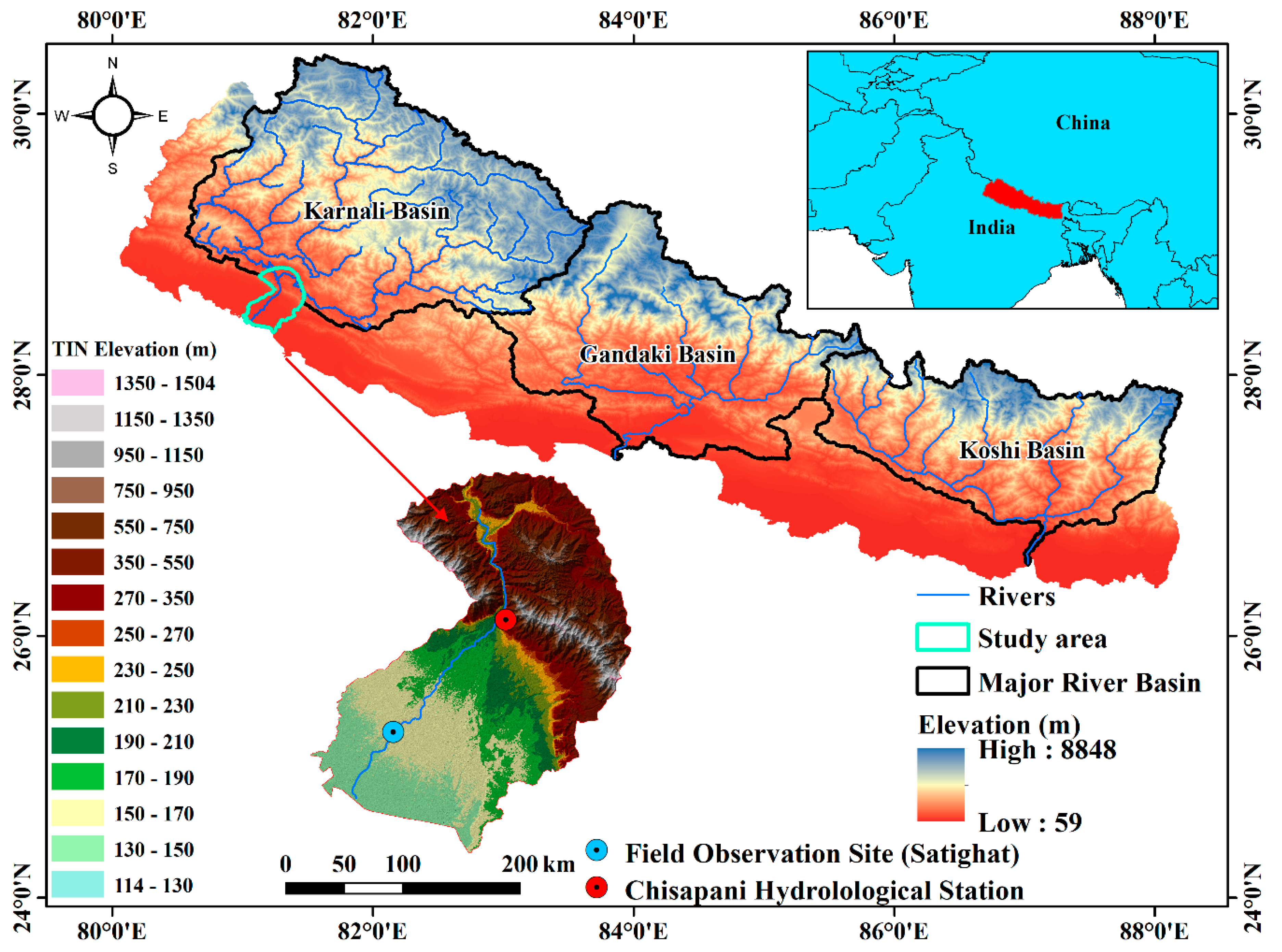
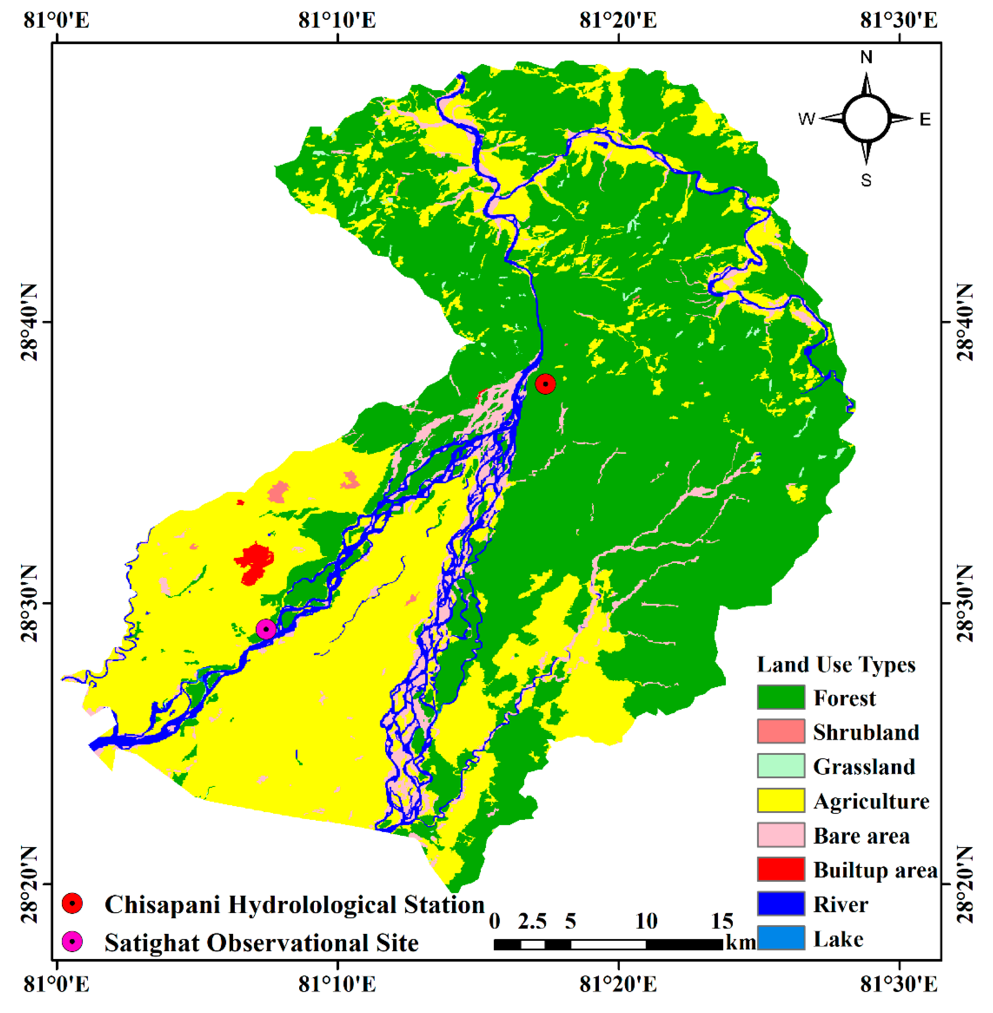
2.1. Study Area
2.2. Data Sets
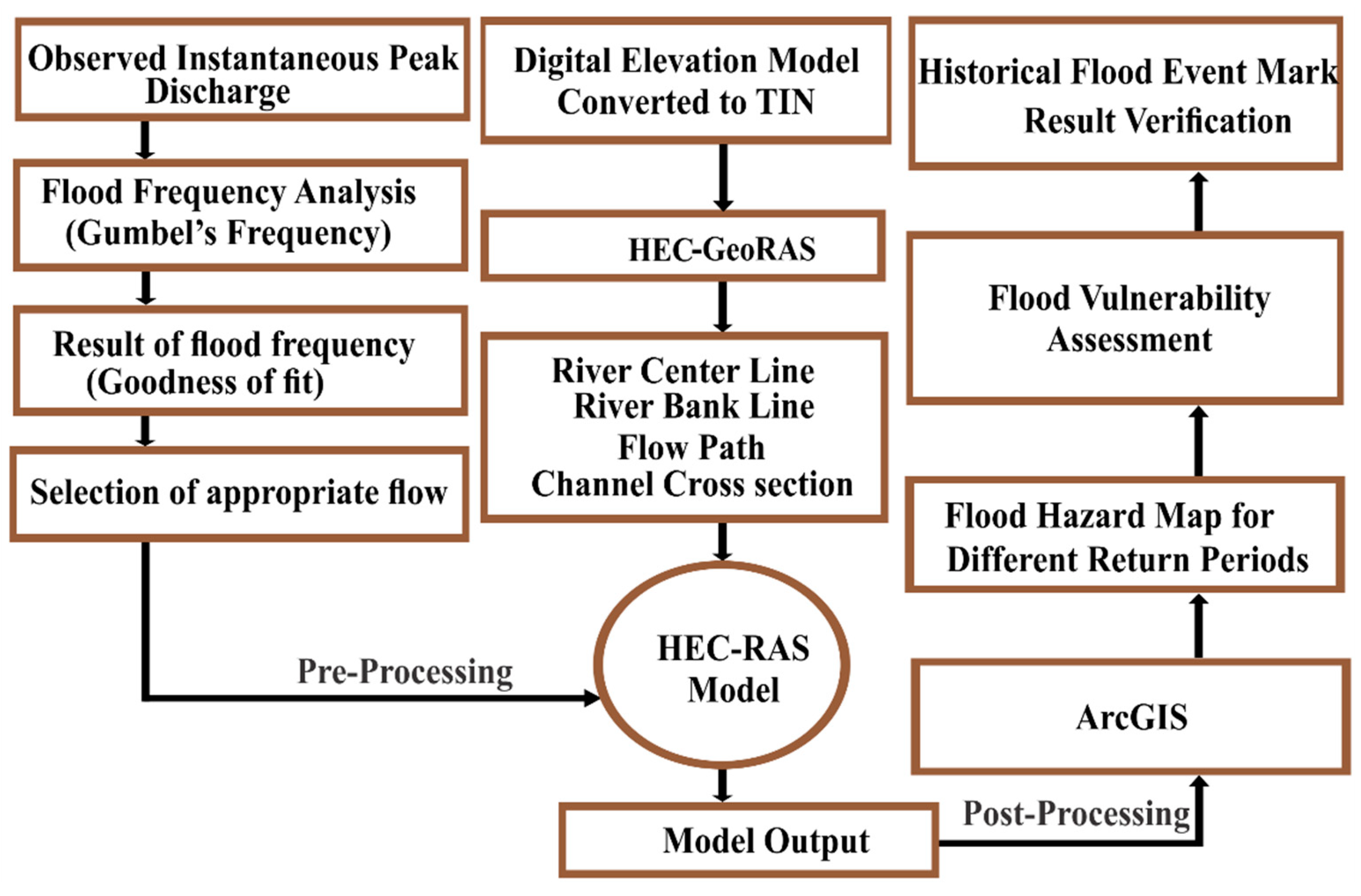
2.3. Methodology
2.4. Model Configuration
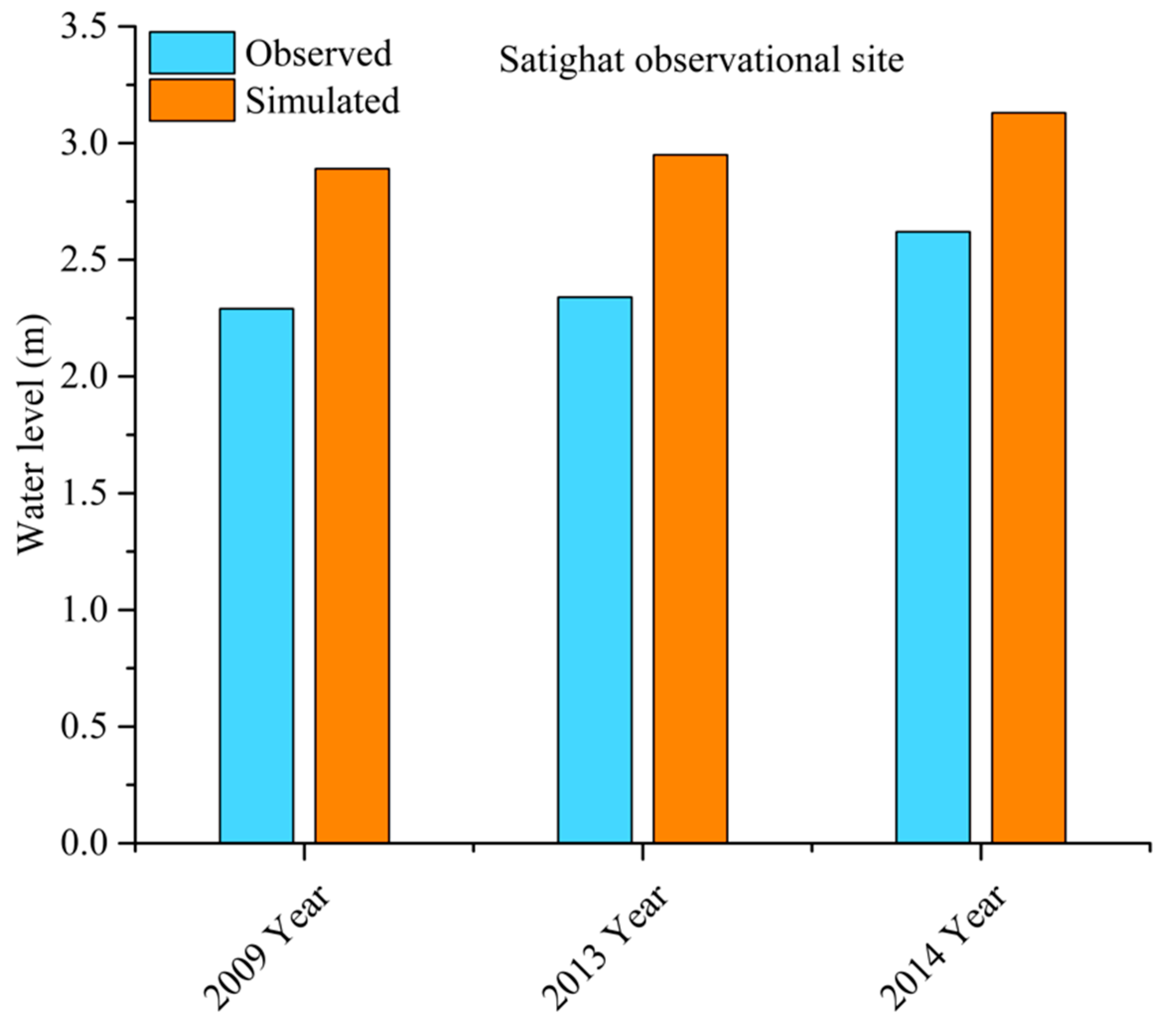
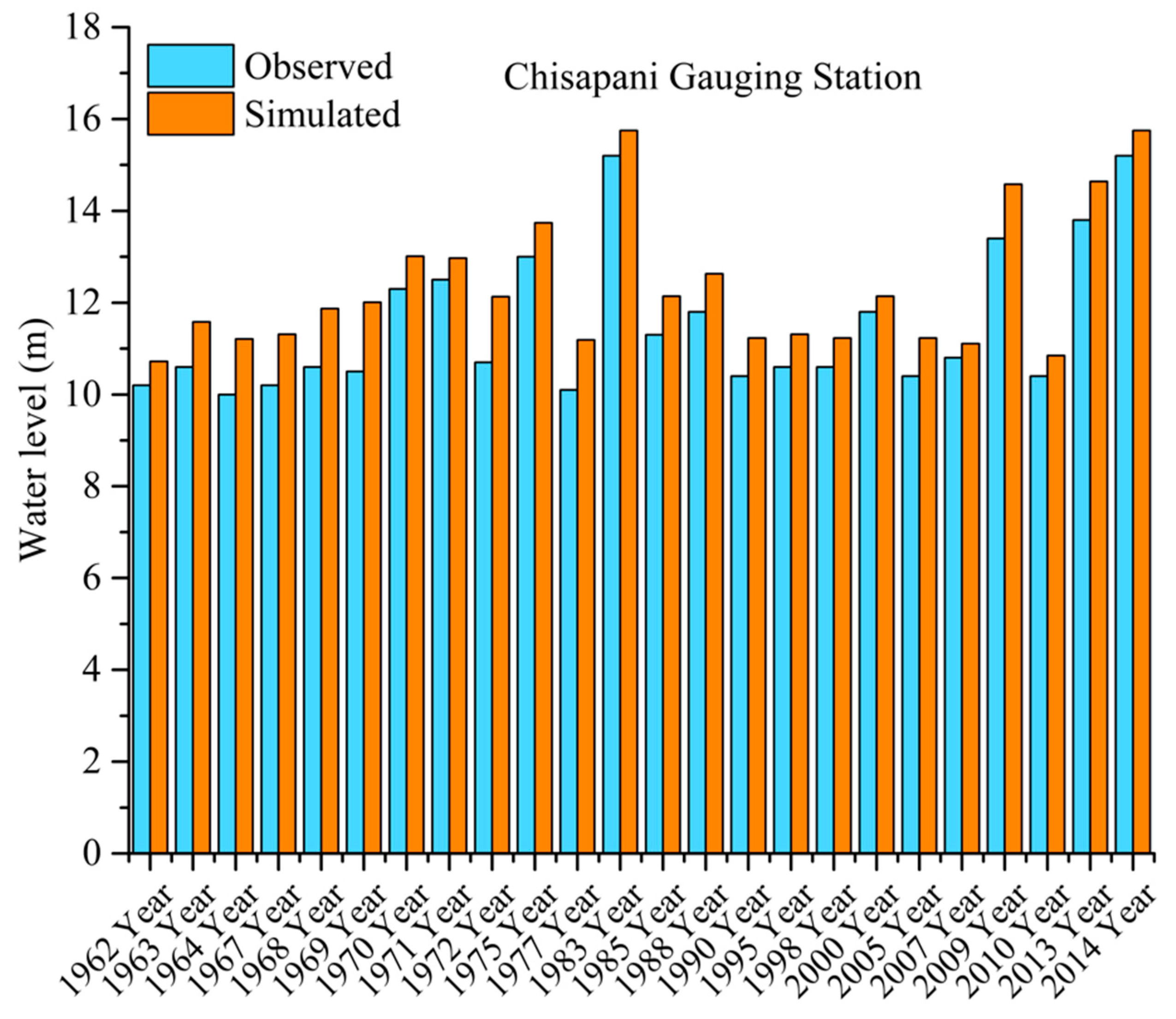
2.5. Model Calibration and Validation
3. Results
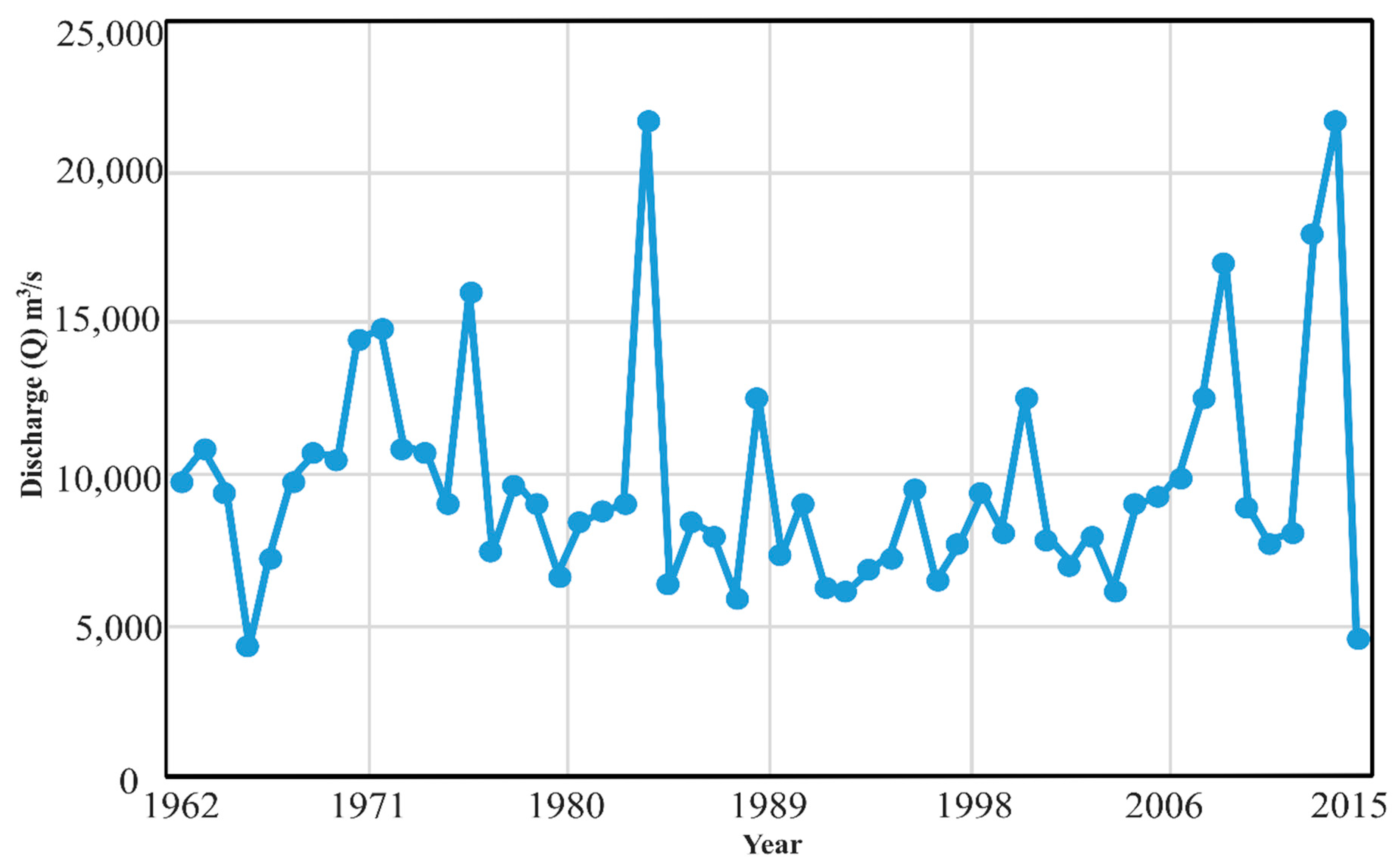
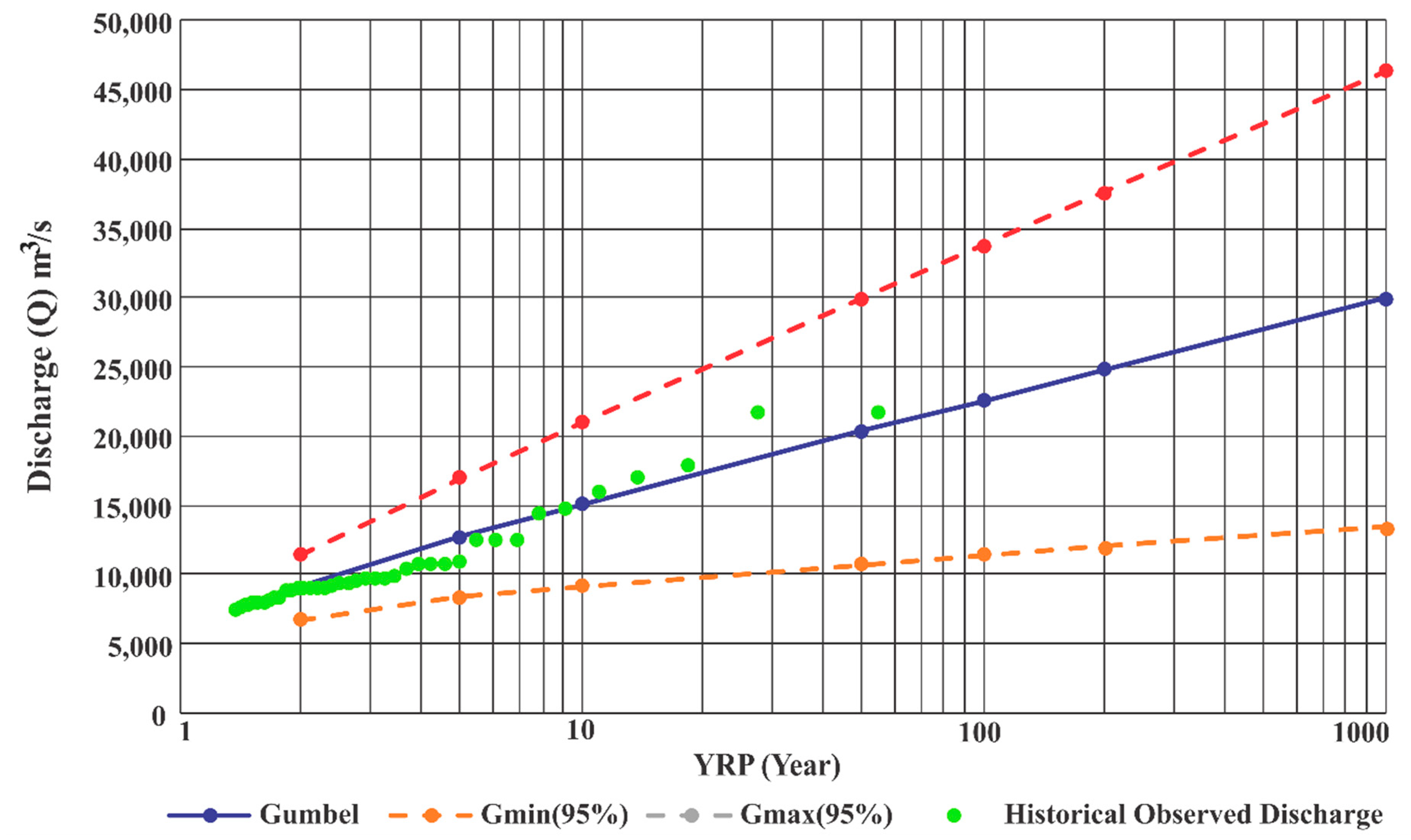
3.1. Flood Frequency Analysis
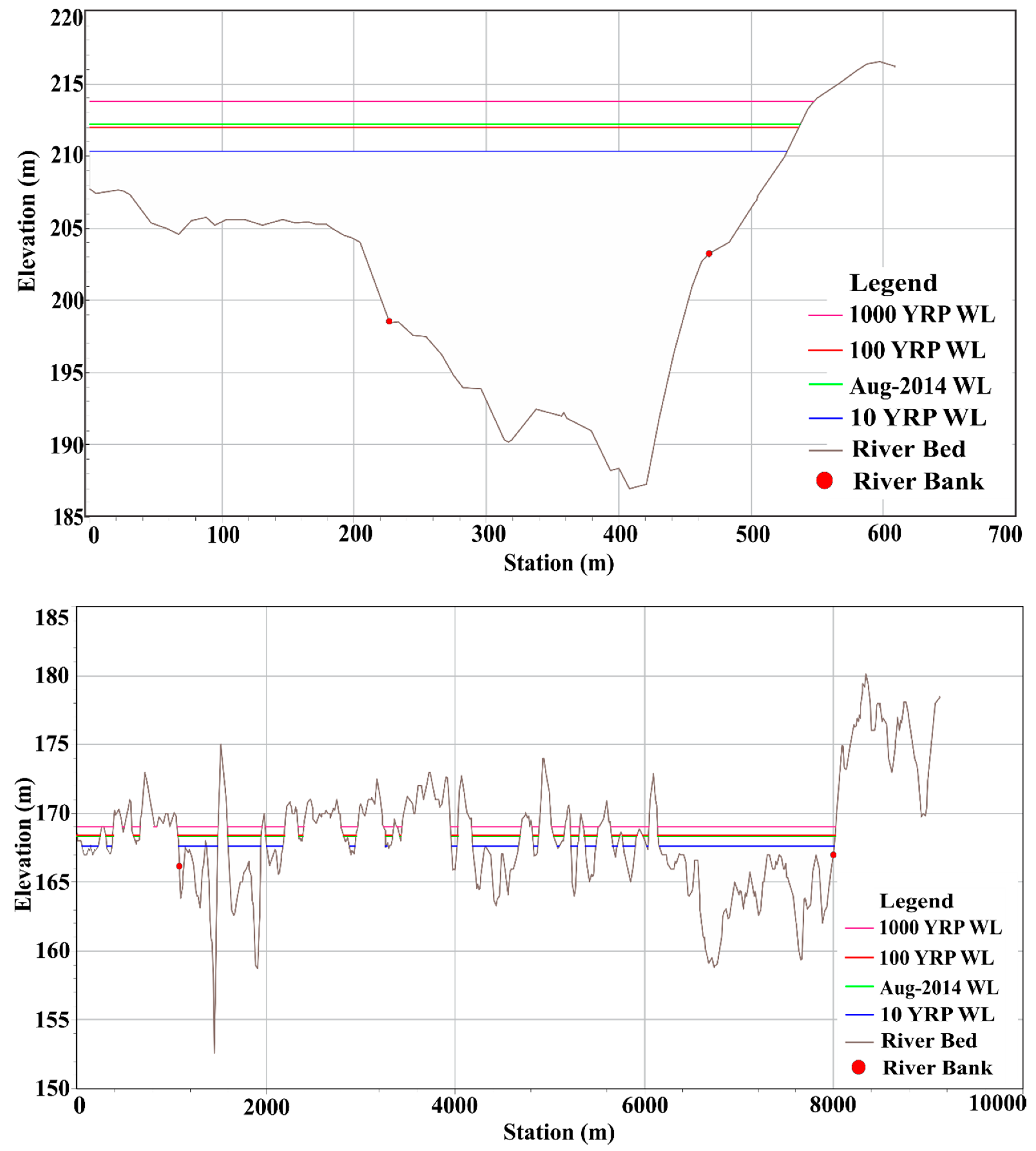
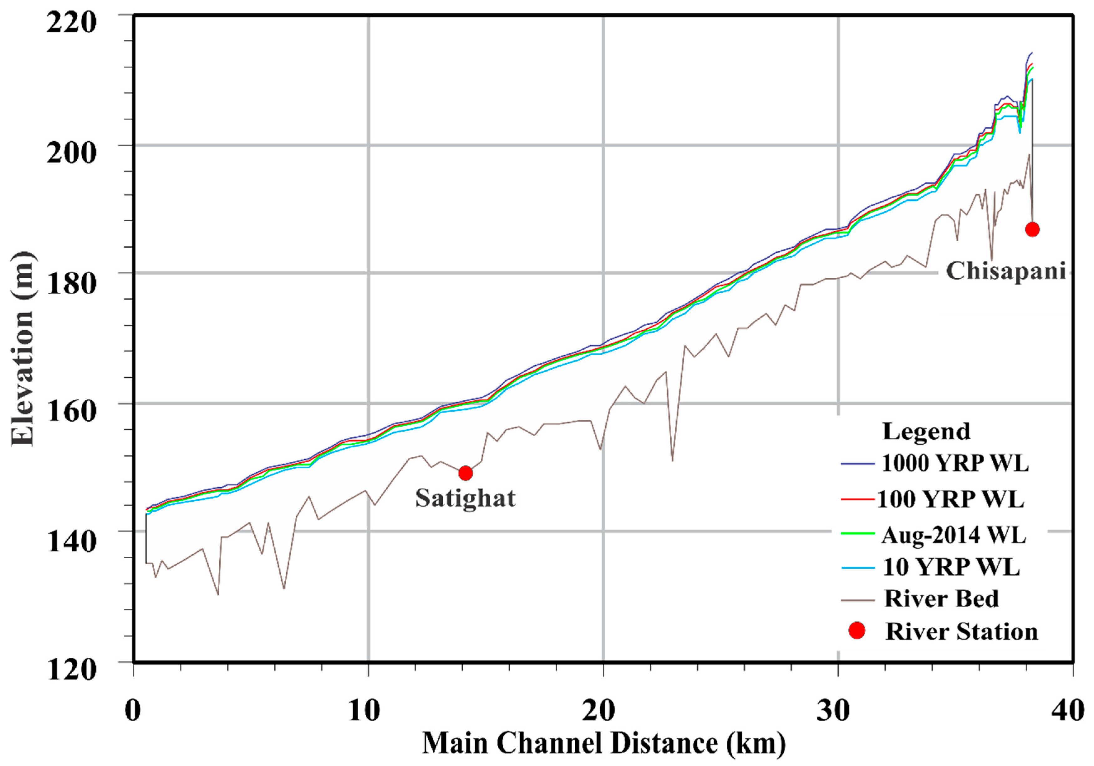
3.2. Comparison and Analysis of Water Surface Profile and Water Surface Elevation
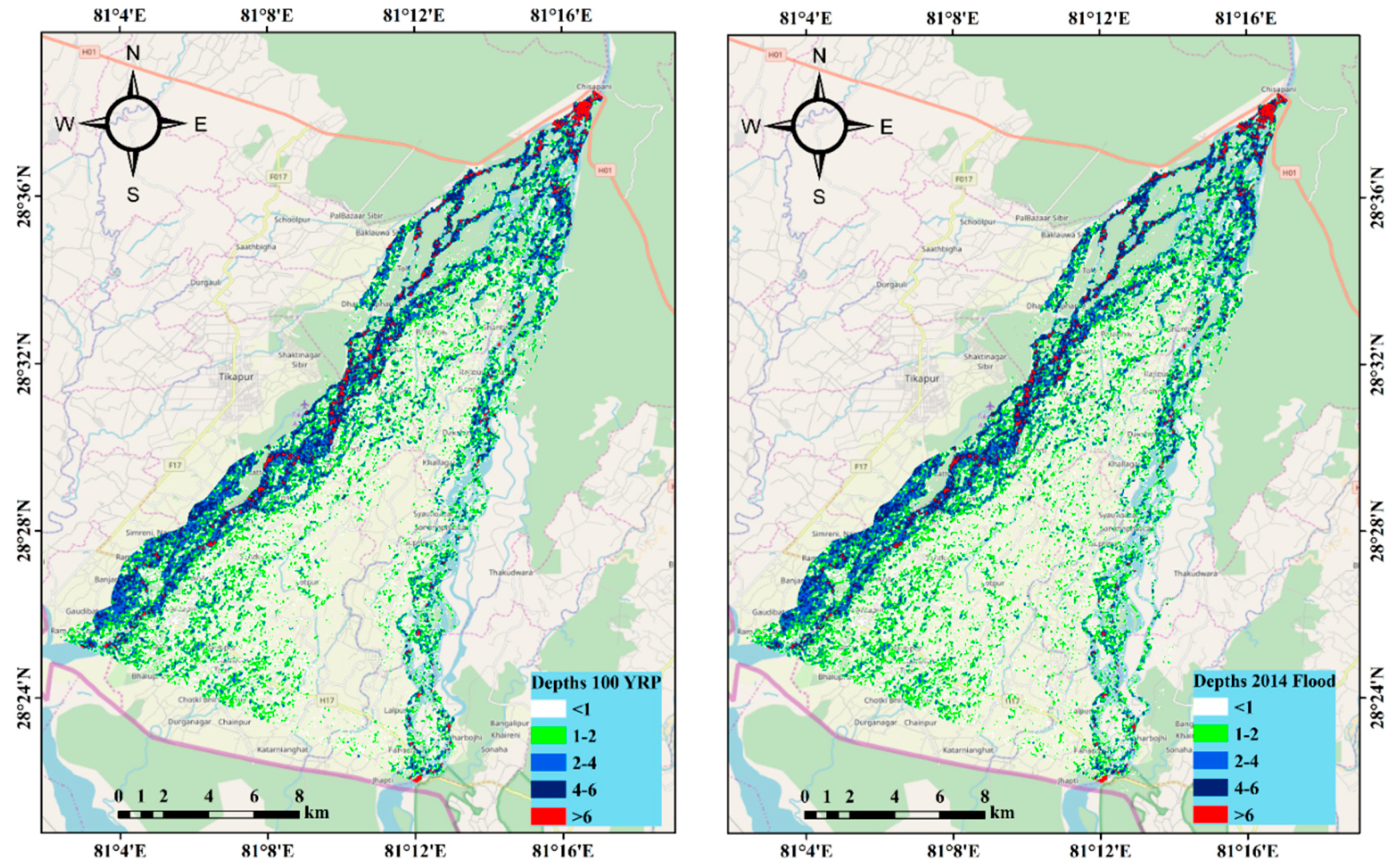
3.3. Simulation of the 2014 Flood Event
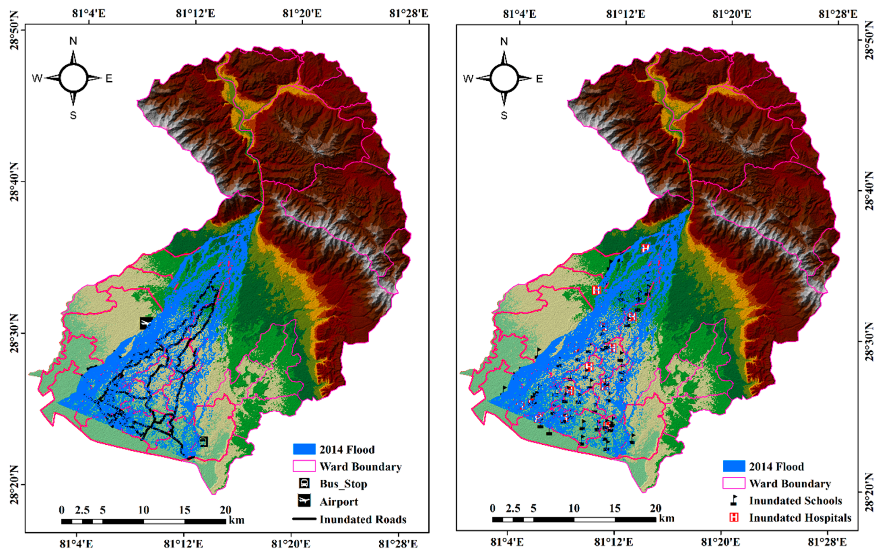
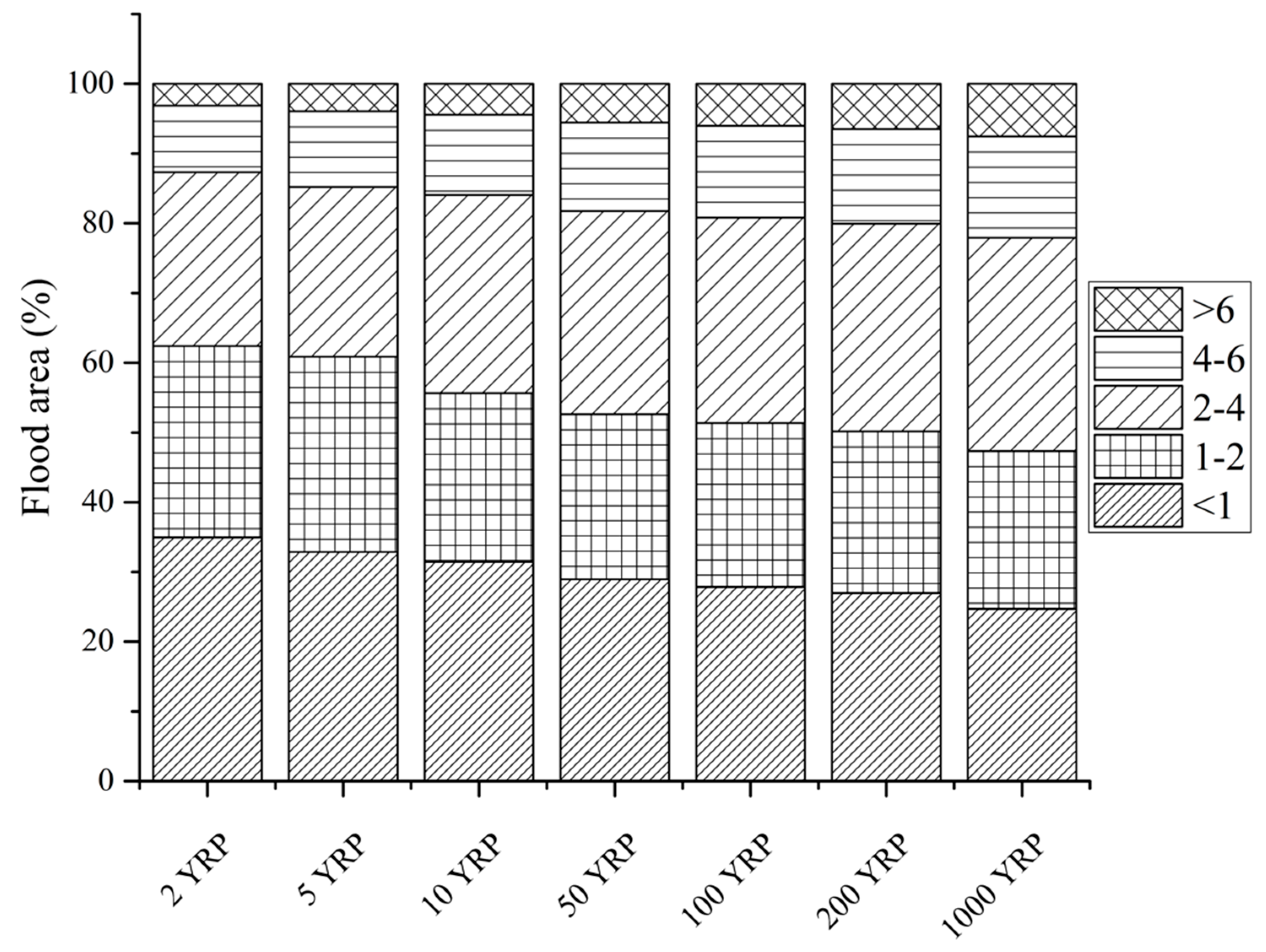
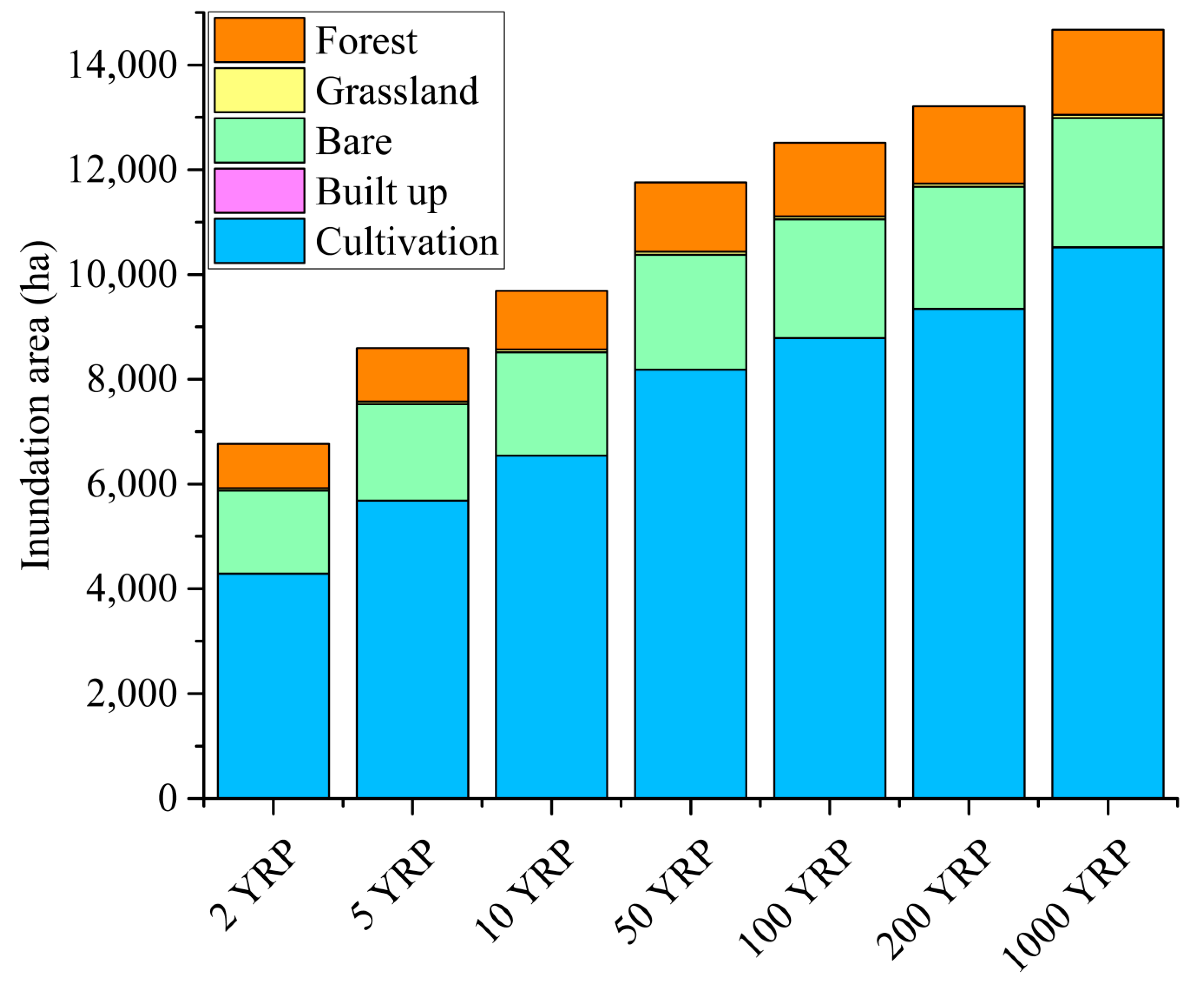
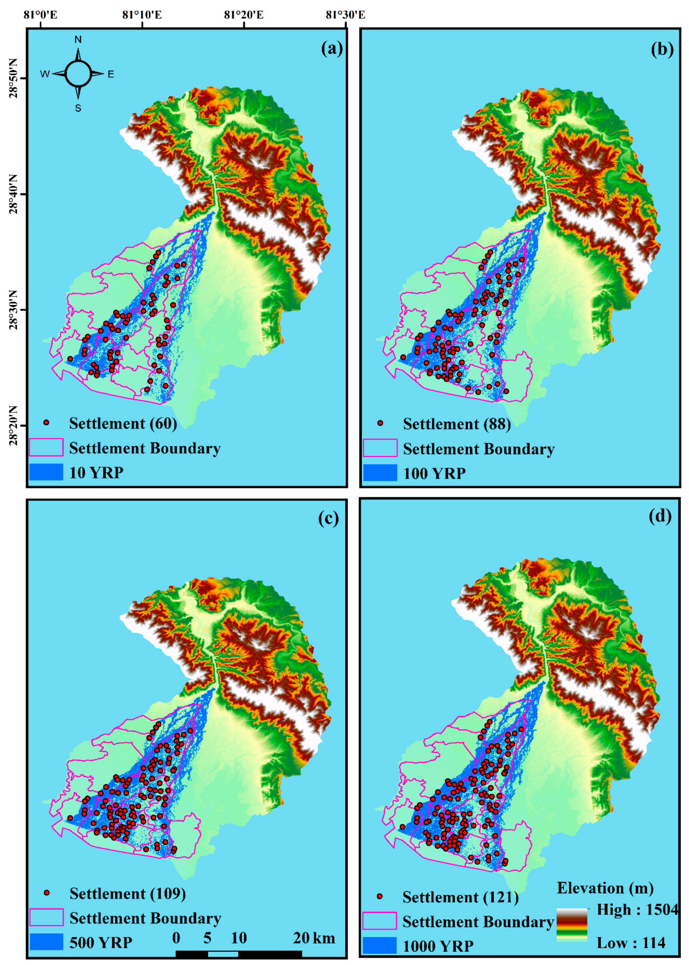
3.4. Flood Hazard Mapping
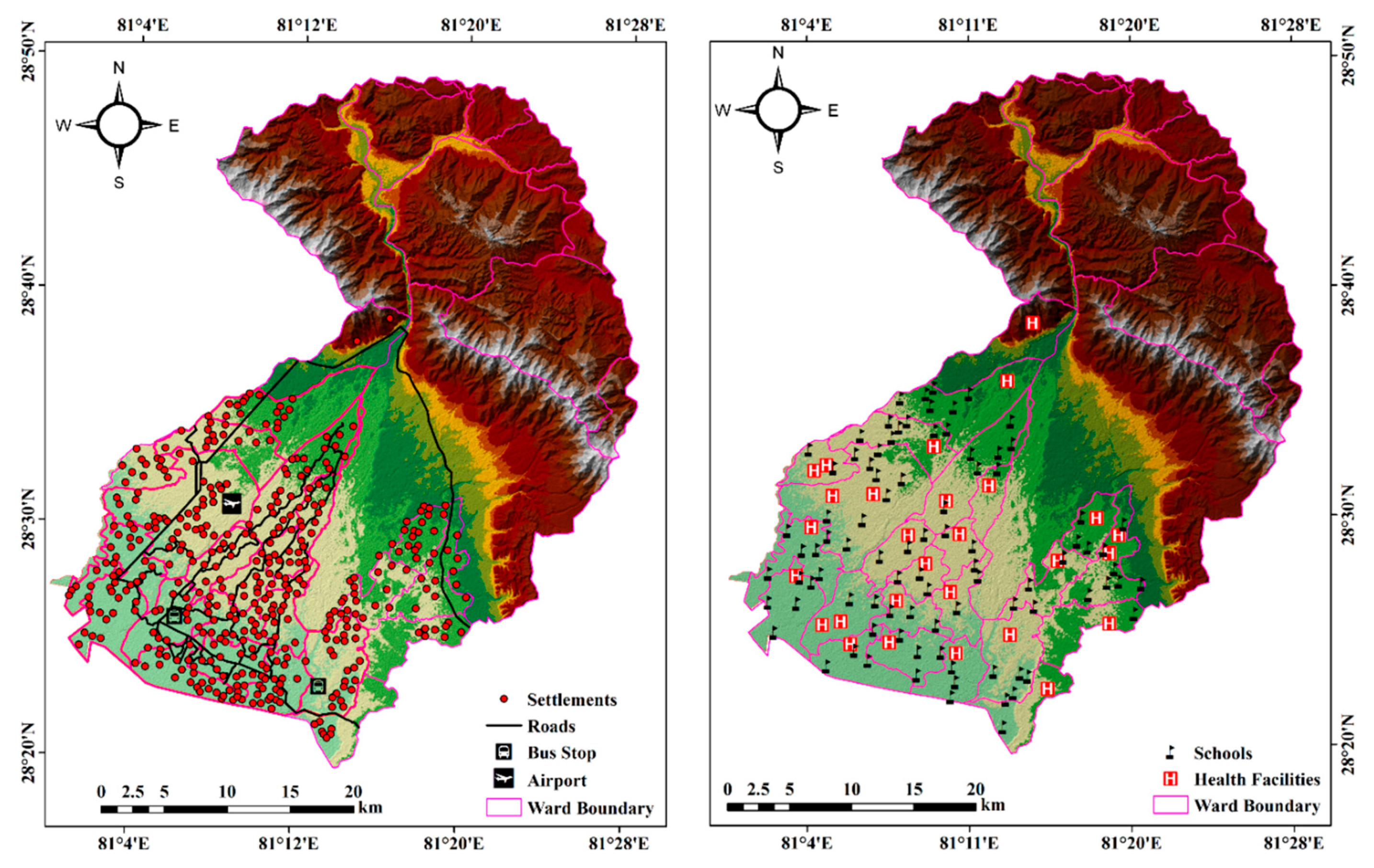
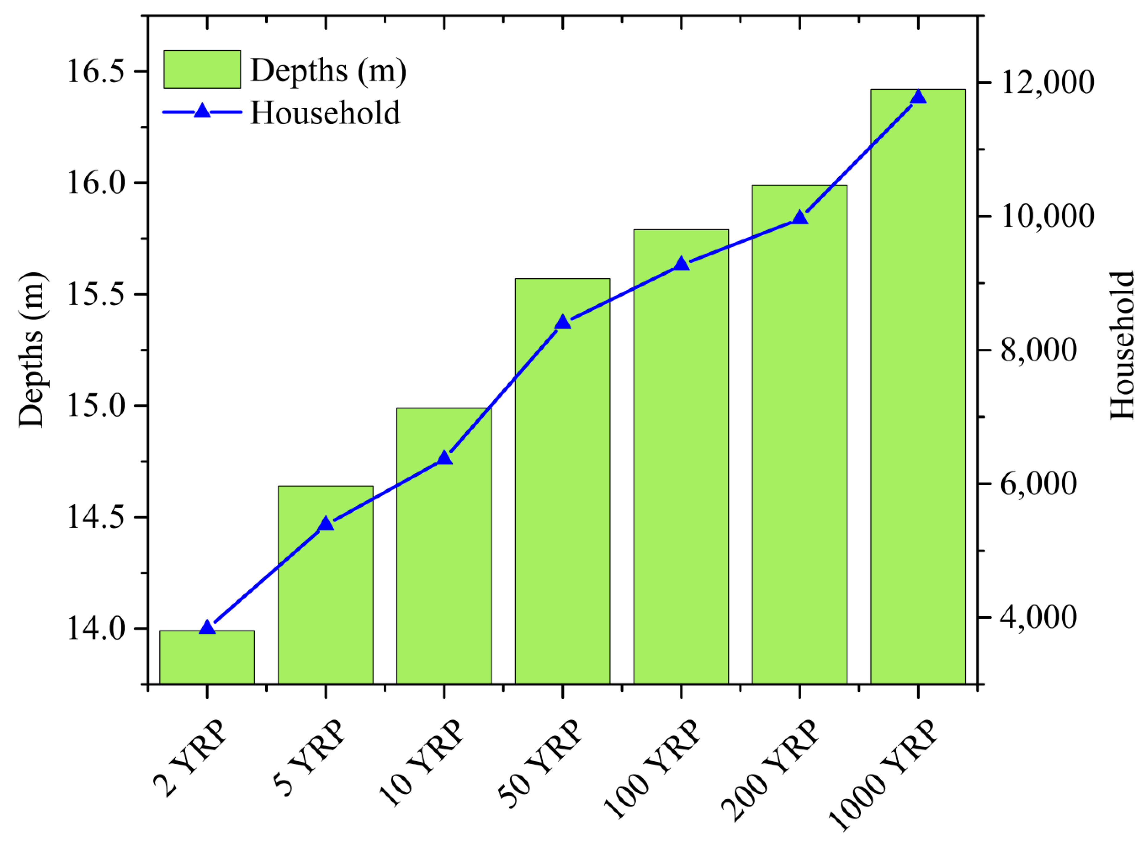
3.5. Flood Vulnerability Assessment
4. Discussion
5. Conclusions
Author Contributions
Funding
Acknowledgments
Conflicts of Interest
References
- Zhao, G.; Xu, Z.; Pang, B.; Tu, T.; Xu, L.; Du, L. An Enhanced Inundation Method for Urban Flood Hazard Mapping at the Large Catchment Scale. J. Hydrol. 2019, 571, 873–882. [Google Scholar] [CrossRef]
- Mcphillips, L.E.; Chang, H.; Chester, M.V.; Depietri, Y. Defining Extreme Events: A Cross-Disciplinary Review Earth ’ s Future Defining Extreme Events: A Cross-Disciplinary Review. Earth’s Future 2018, 6, 1–15. [Google Scholar] [CrossRef]
- Zhang, C.; Wang, Y.; Zhang, L.; Zhou, H. A Fuzzy Inference Method Based on Association Rule Analysis with Application to River Flood Forecasting. Water Sci. Technol. 2012, 66, 2090–2098. [Google Scholar] [CrossRef]
- Yerramilli, S. A Hybrid Approach of Integrating HEC-RAS and GIS towards the Identification and Assessment of Flood Risk Vulnerability in the City of Jackson. Am. J. Geogr. Inf. Syst. 2012, 1, 7–16. [Google Scholar] [CrossRef] [Green Version]
- Botzen, W.J.W.; van den Bergh, J.C.J.M.; Bouwer, L.M. Climate Change and Increased Risk for the Insurance Sector: A Global Perspective and an Assessment for the Netherlands. Nat. Hazards 2010, 52, 577–598. [Google Scholar] [CrossRef] [Green Version]
- Reggiani, P.; Weerts, A.H. A Bayesian Approach to Decision-Making under Uncertainty: An Application to Real-Time Forecasting in the River Rhine. J. Hydrol. 2008, 356, 56–69. [Google Scholar] [CrossRef]
- Dulal, K.N.; Takeuchi, K.; Ishidaira, H. Evaluation of the Influence of Uncertainty in Rainfall and Discharge Data on Hydrological Modeling. Annu. J. Hydraul. Eng. 2007, 51, 31–36. [Google Scholar] [CrossRef] [Green Version]
- Hirabayashi, Y.; Mahendran, R.; Koirala, S.; Konoshima, L.; Yamazaki, D.; Watanabe, S.; Kim, H.; Kanae, S. Global Flood Risk under Climate Change. Nat. Clim. Chang. 2013, 3, 816–821. [Google Scholar] [CrossRef]
- Pandey, G.R.; Nguyen, V.T.V. A Comparative Study of Regression Based Methods in Regional Flood Frequency Analysis. J. Hydrol. 1999, 225, 92–101. [Google Scholar] [CrossRef]
- Wasko, C.; Sharma, A. Global Assessment of Flood and Storm Extremes with Increased Temperatures. Sci. Rep. 2017, 1–8. [Google Scholar] [CrossRef] [PubMed]
- Ibrahim, N.F. Identification of Vulnerable Areas to Floods in Kelantan River Sub-Basins By Using Flood Vulnerability Index. Int. J. Geomate 2016, 12, 107–114. [Google Scholar] [CrossRef]
- Jongman, B.; Ward, P.J.; Aerts, J.C.J.H. Global Exposure to River and Coastal Flooding: Long Term Trends and Changes. Global Environ. Chang. 2012, 22, 823–835. [Google Scholar] [CrossRef]
- Chang, L.F.; Lin, C.H.; Su, M.D. Application of Geographic Weighted Regression to Establish Flood-Damage Functions Reflecting Spatial Variation. Water SA 2008, 34, 209–216. [Google Scholar] [CrossRef] [Green Version]
- Kafle, S. Disaster Risk Management Systems in South Asia: Natural Hazards, Vulnerability, Disaster Risk and Legislative and Institutional Frameworks. J. Geogr. Nat. Disasters 2017, 7. [Google Scholar] [CrossRef]
- Kron, W. Flood Risk = Hazard Values Vulnerability. Water Int. 2005, 30, 58–68. [Google Scholar] [CrossRef]
- Ministry of Home Affairs (MOHA). Nepal Disaster Report, 2017: The Road to Sendai; Government of Nepal: Kathmandu, Nepal, 2018; pp. 1–92.
- Devkota, B.D.; Paudel, P.; Kubota, T.; Deepak, K.C. Landslide and Flood Hazards Consequences and Community Based Management Initiatives in Nepal Himalaya. In Proceedings of the Interpraevent International Symposium, Nara, Japan, 25–28 November 2014. [Google Scholar]
- Department of Water Induced Disaster Prevention (DWIDP). Nepal Disaster Report; Ministry of Home Affairs (MoHA), Government of Nepal, and Disaster Preparedness Network- Nepal (DPNet-Nepal): Kathmandu, Nepal, 2013; pp. 1–108.
- Rasmy, M.; Sayama, T.; Koike, T. Development of Water and Energy Budget-Based Rainfall-Runoff-Inundation Model (WEB-RRI) and Its Verification in the Kalu and Mundeni River Basins, Sri Lanka. J. Hydrol. 2019, 579, 1–23. [Google Scholar] [CrossRef]
- Gaire, S.; Delgado, R.C.; Gonzalez, P.A. Disaster Risk Profile and Existing Legal Framework of Nepal: Floods and Landslides. Risk Manag. Healthc. Policy 2015, 139–149. [Google Scholar] [CrossRef] [Green Version]
- Devi, N.N.; Sridharan, B.; Kuiry, S.N. Impact of Urban Sprawl on Future Flooding in Chennai City, India Impact of Urban Sprawl on Future Flooding in Chennai City, India. J. Hydrol. 2019, 574, 486–496. [Google Scholar] [CrossRef]
- Schumann, G.J.; Neal, J.C.; Voisin, N.; Andreadis, K.M.; Pappenberger, F.; Phanthuwongpakdee, N.; Hall, A.C.; Bates, P.D. A First Large-Scale Flood Inundation Forecasting Model. Water Resour. Res. 2013, 49, 6248–6257. [Google Scholar] [CrossRef]
- Horritt, M.S.; Bates, P.D. Evaluation of 1D and 2D Numerical Models for Predicting River Flood Inundation. J. Hydrol. 2002, 268, 87–99. [Google Scholar] [CrossRef]
- Horritt, M.S.; Bates, P.D. Predicting Floodplain Inundation: Raster-Based Modelling versus the Finite-Element Approach. Hydrol. Process. 2001, 15, 825–842. [Google Scholar] [CrossRef]
- Bates, P.D.; Roo, A.P.J.D. A Simple Raster-Based Model for Flood Inundation Simulation. J. Hydrol. 2000, 236, 54–77. [Google Scholar] [CrossRef]
- Brunner, G.W. HEC-RAS, River Analysis System Hydraulic Reference Manual; US Army Corps of Engineers Hydrologic Engineering Center: Davis, CA, USA, 2016; pp. 1–547. [Google Scholar]
- Liu, Z.; Merwade, V.; Jafarzadegan, K. Investigating the Role of Model Structure and Surface Roughness in Generating Flood Inundation Extents Using One- and Two- Dimensional Hydraulic Models. J. Flood Risk Manag. 2019, 1–19. [Google Scholar] [CrossRef] [Green Version]
- Romali, N.S. Application of Hec-Ras and Arc Gis for Floodplain Mapping in Segamat Town, Malaysia. Int. J. Geomate 2018, 14. [Google Scholar] [CrossRef]
- Golshana, M.; Afzali, A.; Jahanshahia, A. Flood Hazard Zoning Using HEC-RAS in GIS Environment and Impact of Manning Roughness Coefficient Changes on Flood Zones in Semi-Arid Climate. Desert 2016, 1, 24–34. [Google Scholar]
- Patel, C.G.; Gundaliya, P.J. Floodplain Delineation Using HECRAS Model—A Case Study of Surat City. Open J. Mod. Hydrol. 2016, 6, 34–42. [Google Scholar] [CrossRef] [Green Version]
- Yang, J.; Townsend, R.D.; Daneshfar, B. Applying the HEC-RAS Model and GIS Techniques in River Network Floodplain Delineation. Candian J. Civ. Eng. 2006, 33, 19–28. [Google Scholar] [CrossRef]
- Earles, T.A.; Wright, K.R.; Brown, C.; Langan, T.E. Los Alamos Forest Fire Impact Modeling. J. Am. Water J. Am. Water Resour. Assoc. 2004, 40, 371–384. [Google Scholar] [CrossRef]
- Adhikari, K. Modelling and Simulation of Floods in Barsa River near Pasakha, Bhutan. In Proceedings of the Conference on ‘Climate Change, Environment and Development in Bhutan, Thimphu, Bhutan, 2–3 April 2015; Thinley, S.U., Ed.; Royal University of Bhutan (RUB): Thimpu, Bhutan; pp. 79–84. [Google Scholar]
- Azouagh, A.; El Bardai, R.; Hilal, I.; Stitou el Messari, J. Integration of GIS and HEC-RAS in Floods Modeling of Martil River (Northern Morocco). Eur. Sci. J. 2018, 14, 130. [Google Scholar] [CrossRef]
- Mai, D.T.; De Smedt, F. A Combined Hydrological and Hydraulic Model for Flood Prediction in Vietnam Applied to the Huong River Basin as a Test Case Study. Water 2017, 9, 879. [Google Scholar] [CrossRef] [Green Version]
- Dangol, S.; Bormudoi, A. Flood Hazard Mapping and Vulnerability Analysis of Bishnumati River, Nepal. Nepal. J. Geoinform. Survey Dep. Nepal 2015, 14, 20–24. [Google Scholar]
- Dangol, S. Use of Geo-Informatics in Flood Hazard Mapping: A Case of Balkhu River. Nepal. J. Geoinform. Survey Dep. Nepal 2014, 13, 52–57. [Google Scholar]
- Talchabhadel, R.; Shakya, N.M.; Dahal, V.; Eslamian, S. Rainfall Runoff Modelling for Flood Forecasting (a Case Study on West Rapti Watershed). J. Flood Eng. 2015, 6, 53–61. [Google Scholar]
- Gautam, D.K.; Phaiju, A.G. Community Based Approach to Flood Early Warning in West Rapti River Basin of Nepal. J. Integr. Disaster Risk Manag. 2013, 3, 155–169. [Google Scholar] [CrossRef]
- Cook, E.R.; Krusic, P.J.; Jones, P.D. Dendroclimatic Signals in Long Tree-Ring Chronologies from the Himalayas of Nepal. Int. J. Climatol. 2003, 732, 707–732. [Google Scholar] [CrossRef]
- Dixit, A.M.; Gremli, R. Risk Nexus; Urgent Case for Recovery: What We Can Learn from the August 2014 Karnali River Floods in Nepal; Technical Report. Zurich Insurance Group Ltd: Zurich, Switzerland; ISET-International: Boulder, CO, USA, 2015; pp. 1–44. [Google Scholar] [CrossRef]
- Ministry of Water Resource (MOWR). Master Plan Study for Water Resources Development of the Upper Karnali River and Mahakali River Basins; Japan International Cooperation Agency: Tokyo, Japan, 1993.
- Khadka, N.; Zhang, G.; Thakuri, S. Glacial Lakes in the Nepal Himalaya: Inventory and Decadal Dynamics (1977–2017). Remote Sens. 2018, 10, 1913. [Google Scholar] [CrossRef] [Green Version]
- Dulal, H.B.; Brodnig, G.; Thakur, H.K.; Green-Onoriose, C. Do the Poor Have What They Need to Adapt to Climate Change? A Case Study of Nepal. Local Environ. 2010, 15, 621–635. [Google Scholar] [CrossRef]
- Malla, G. Climate Change and Its Impact on Nepalese Agriculture. J. Agric. Environ. 2008, 9, 62–71. [Google Scholar] [CrossRef] [Green Version]
- Talchabhadel, R.; Karki, R.; Thapa, B.R.; Maharjan, M. Spatio-Temporal Variability of Extreme Precipitation in Nepal. Int. J. Climatol. 2018, 1–18. [Google Scholar] [CrossRef]
- Department of Hydrology and Meteorology (DHM). Observed Climate Trend Analysis in the Districts and Physiographic Regions of Nepal (1971–2014); Department of Hydrology and Meteorology: Kathmandu, Nepal, 2017; pp. 1–101. [CrossRef]
- Shrestha, M.L. Interannual Variation of Summer Monsoon Rainfall over Nepal and Its Relation to Southern Oscillation Index. Meteorol. Atmos. Phys. 2000, 75, 21–28. [Google Scholar] [CrossRef]
- Shrestha, B.; Ye, Q.; Khadka, N. Assessment of Ecosystem Services Value Based on Land Use and Land Cover Changes in the Transboundary Karnali River Basin, Central Himalayas. Sustainability 2019, 11, 3183. [Google Scholar] [CrossRef] [Green Version]
- Khatiwada, K.; Panthi, J.; Shrestha, M.; Nepal, S. Hydro-Climatic Variability in the Karnali River Basin of Nepal Himalaya. Climate 2016, 4, 17. [Google Scholar] [CrossRef]
- Water and Energy Commission Secretariat (WECS). National Water Plan; Ministry of Water Resources: Kathmandu, Nepal, 2005; pp. 1–97.
- SRTM 30m DEM, Digital Elevation Model Database; United States Geological Survey (USGS): Reston, VA, USA. Available online: https://earthexplorer.usgs.gov/ (accessed on 12 January 2019).
- Bajracharya, S. Land Cover of Nepal 2010; International Centre for Integrated Mountain Development: Lalitpur, Nepal, 2010. [Google Scholar] [CrossRef]
- Geofabrik Software Development Company, Germany. Open Street Map Contributors, Creative Commons. Mountain View, CA, USA. Available online: https://download.geofabrik.de/asia/nepal.html/ (accessed on 12 January 2019).
- Central Bureau of Statistics (CBS). National Population and Housing Census 2011 (Village Development Committee/Municipality) Central Bureau of Statistics; Government of Nepal: Kathmandu, Nepal, 2011; Volume 2, pp. 1–108.
- Husain, A.; Sharif, M.; Ahmad, M.L. Simulation of Floods in Delhi Segment of River Yamuna Using HEC-RAS. Am. J. Water Resour. 2018, 6, 162–168. [Google Scholar] [CrossRef]
- Gumbel, E.J. Statistics of Extremes, 1st ed.; Dover Publications, Inc.: Mineola, NY, USA, 1958; pp. 1–373. ISBN 0486154483. [Google Scholar]
- Chow Te, V.; Maidment, D.R.; Mays, L.W. Applied-Hydrology; McGraw-Hill Book Company: New York, NY, USA, 1988; pp. 1–565. [Google Scholar]
- Ang, A.H.-S.; Tang, W.H. Probability Concepts in Engineering Planning and Design, Volume-2, Basic Principles. In Decision, Risk, and Reliability; John Wiley & Sons Inc.: Hoboken, NJ, USA, 1984; Volume 608. [Google Scholar]
- Farr, T.G.; Rosen, P.A.; Caro, E.; Crippen, R.; Duren, R.; Hensley, S.; Kobrick, M.; Paller, M.; Rodriguez, E.; Roth, L.; et al. The Shuttle Radar Topography Mission. Rev. Geophys. 2007, 45, 1–44. [Google Scholar] [CrossRef] [Green Version]
- Barnes, H.H. Roughness Characteristics of Natural Channels; United States Government Printing Office: Washington, DC, USA, 1967; pp. 1–211. [Google Scholar]
- Lamichhane, N.; Sharma, S. Effect of Input Data in Hydraulic Modeling for Flood Warning Systems. Hydrolological Sci. J. 2018, 63, 938–956. [Google Scholar] [CrossRef]
- Aryal, U.; Adhikari, T.R.; Thakuri, S.; Rakhal, B. Flood Hazard Assessment in Dhobi-Khola Watershed, (Kathmandu Nepal) Using Hydrological Model. Int. Res. J. Environ. Sci. 2016, 5, 21–33. [Google Scholar]
- Merz, B.; Thieken, A.H.; Gocht, M. Flood Risk Mapping at the Local Scale: Concepts and Challenges. Adv. Nat. Technol. Hazards Res. 2007, 25, 231–251. [Google Scholar] [CrossRef]
- Leedal, D.; Neal, J.; Beven, K.; Young, P.; Bates, P. Visualization Approaches for Communicating Real-Time Flood Forecasting Level and Inundation Information. J. Flood Risk Manag. 2010, 3, 140–150. [Google Scholar] [CrossRef]
- Hicks, F.E.; Peacock, T. Suitability of HEC-RAS for Flood Forecasting. Can. Water Resour. J. 2005, 30, 159–174. [Google Scholar] [CrossRef]
- Gautam, D.K.; Dulal, K. Determination of Threshold Runoff for Flood Warning in Nepalese Rivers. J. Integr. Disaster Risk Manag. 2013, 3, 125–136. [Google Scholar] [CrossRef] [Green Version]
- Dartmouth Flood Observatory. Global Active Archive of Large Flood Events. Available online: http://www.dartmouth.edu/~floods/Archives/index.html/ (accessed on 12 January 2019).
- Shrestha, M.S.; Heggen, R.; Thapa, K.; Ghimire, M.L.; Shakya, N. Flood Risk and Vulnerability Mapping Using GIS: A Nepal Case Study. In Proceedings of the Asia Pacific Association of Hydrology and Water Resources, Second APHW Conference, Singapore, 5–8 July 2004; pp. 1–10. [Google Scholar]
- Dixit, A.; Gyawali, D.; Upadhya, M.; Pokhrel, A.; Khan, F.; Optiz-Stapleton, D.S.; New, D.M.; Lizcano, G.; McSweeney, C.; Rahiz, M.; et al. Vulnerability Through the Eyes of the Vulnerable: Climate Change Induced Uncertainties and Nepal’s Development Predicaments; Nepal Climate Vulnerability Study Team, Institute for Social and Environmental Transition-Nepal (ISET-N) and Institute for Social and Environmental Transition (ISET): Boulder, CO, USA, 2009; pp. 1–96. [Google Scholar]
- Adhikari, B.R. Flooding and Inundation in Nepal Terai: Issues and Concerns. Hydro Nepal 2013, 12, 59–65. [Google Scholar] [CrossRef] [Green Version]
- Karki, R.; Hasson ul, S.; Gerlitz, L.; Talchabhadel, R.; Schenk, E.; Schickhoff, U.; Scholten, T.; Böhner, J. WRF-Based Simulation of an Extreme Precipitation Event over the Central Himalayas: Atmospheric Mechanisms and Their Representation by Microphysics Parameterization Schemes. Atmos. Res. 2018, 214, 21–35. [Google Scholar] [CrossRef]
- World Meteorological Organization (WMO). Estimation of Maximum Floods. Report of a Working Group of the Commission for Hydrometeorology; WMO-No. 233.TP.126 Secretariat of the World Meteorological Organization (WHO): Geneva, Switzerland, 1969; pp. 1–288. [Google Scholar]
- Khattak, M.S.; Anwar, F.; Saeed, T.U.; Sharif, M.; Sheraz, K.; Ahmed, A. Floodplain Mapping Using HEC-RAS and ArcGIS: A Case Study of Kabul River. Arab. J. Sci. Eng. 2016, 41, 1375–1390. [Google Scholar] [CrossRef]
- Jonkman, S.N.; Vrijling, J.K.; Vrouwenvelder, A.C.W.M. Methods for the Estimation of Loss of Life Due to Floods: A Literature Review and a Proposal for a New Method. Nat. Hazards 2008, 46, 353–389. [Google Scholar] [CrossRef] [Green Version]
- Samarasinghe, S.; Nandalal, H.; Weliwitiya, D.; Fowze, J.; Harazika, M.; Samarakoon, L. Application of Remote Sensing and GIS for Flood Risk Analysis:A Case Study at Kalu - Ganga River, Sri Lanka. Int. Arch. Photogramm. Remote Sens. Spat. Inf. Sci. 2010, 8, 110–115. [Google Scholar]


| Year | 1985–1990 | 1990–1995 | 1995–2000 | 2000–2005 | 2005–2010 | 2010–2015 | 2015–2020 |
|---|---|---|---|---|---|---|---|
| Deaths | 243 | 3369 | 426 | 920 | 990 | 417 | 165 |
| Displaced (log10) | 4 | 7 | 4 | 6 | 7 | 5 | 4 |
| No. of Events | 6 | 4 | 6 | 10 | 12 | 7 | 5 |
| Return Period (Tr) | 2 | 5 | 10 | 50 | 100 | 200 | 1000 |
|---|---|---|---|---|---|---|---|
| Minimum | 6748 | 8389 | 9185 | 10,754 | 11,389 | 13,442 | 13,442 |
| Gumbel’s | 9088 | 12,696 | 15,085 | 20,343 | 22,565 | 24,780 | 29,910 |
| Maximum | 11,428 | 17,004 | 20,986 | 29,931 | 33,742 | 46,377 | 46,377 |
| River Name | Station | Threshold by DHM | Remarks | ||
|---|---|---|---|---|---|
| Runoff (m3/s) | Water Level (m) | Reference to MSL | |||
| Karnali | Chisapani | 8200 | 10.0 | 201.64 | Warning Level |
| 10,000 | 10.80 | 202.44 | Danger Level | ||
© 2020 by the authors. Licensee MDPI, Basel, Switzerland. This article is an open access article distributed under the terms and conditions of the Creative Commons Attribution (CC BY) license (http://creativecommons.org/licenses/by/4.0/).
Share and Cite
Aryal, D.; Wang, L.; Adhikari, T.R.; Zhou, J.; Li, X.; Shrestha, M.; Wang, Y.; Chen, D. A Model-Based Flood Hazard Mapping on the Southern Slope of Himalaya. Water 2020, 12, 540. https://doi.org/10.3390/w12020540
Aryal D, Wang L, Adhikari TR, Zhou J, Li X, Shrestha M, Wang Y, Chen D. A Model-Based Flood Hazard Mapping on the Southern Slope of Himalaya. Water. 2020; 12(2):540. https://doi.org/10.3390/w12020540
Chicago/Turabian StyleAryal, Dibit, Lei Wang, Tirtha Raj Adhikari, Jing Zhou, Xiuping Li, Maheswor Shrestha, Yuanwei Wang, and Deliang Chen. 2020. "A Model-Based Flood Hazard Mapping on the Southern Slope of Himalaya" Water 12, no. 2: 540. https://doi.org/10.3390/w12020540
APA StyleAryal, D., Wang, L., Adhikari, T. R., Zhou, J., Li, X., Shrestha, M., Wang, Y., & Chen, D. (2020). A Model-Based Flood Hazard Mapping on the Southern Slope of Himalaya. Water, 12(2), 540. https://doi.org/10.3390/w12020540