Abstract
Although river water quality monitoring (WQM) networks play an important role in water management, their effectiveness is rarely evaluated. This study aims to evaluate and optimize water quality variables and monitoring sites to explain the spatial and temporal variation of water quality in rivers, using principal component analysis (PCA). A complex water quality dataset from the Freiberger Mulde (FM) river basin in Saxony, Germany was analyzed that included 23 water quality (WQ) parameters monitored at 151 monitoring sites from 2006 to 2016. The subsequent results showed that the water quality of the FM river basin is mainly impacted by weathering processes, historical mining and industrial activities, agriculture, and municipal discharges. The monitoring of 14 critical parameters including boron, calcium, chloride, potassium, sulphate, total inorganic carbon, fluoride, arsenic, zinc, nickel, temperature, oxygen, total organic carbon, and manganese could explain 75.1% of water quality variability. Both sampling locations and time periods were observed, with the resulting mineral contents varying between locations and the organic and oxygen content differing depending on the time period that was monitored. The monitoring sites that were deemed particularly critical were located in the vicinity of the city of Freiberg; the results for the individual months of July and September were determined to be the most significant. In terms of cost-effectiveness, monitoring more parameters at fewer sites would be a more economical approach than the opposite practice. This study illustrates a simple yet reliable approach to support water managers in identifying the optimum monitoring strategies based on the existing monitoring data, when there is a need to reduce the monitoring costs.
1. Introduction
Rivers are the main inland freshwater source for domestic, industrial, and agricultural purposes [1]. As a result of the deleterious effects of human activities and population growth, about one-third of the river stretches in Latin America, Africa, and Asia have been affected by severe pathogen contamination, and one-seventh by organic pollution [2]. Additionally, natural processes such as precipitation, erosion, and weathering of crustal materials can also contribute to the impairment of water quality in rivers [1,3]. In European water bodies, the emphasis on chemical water quality assessment has shifted to trace contaminants [4]. As a result, over 50% of all European Union rivers, including all rivers in some countries, fail to achieve a good chemical state [5]. To protect and properly manage the rivers, the monitoring of water quality is critical [6,7]. Water quality monitoring (WQM) is defined as the effort to obtain quantitative information on the physical, chemical, and biological characteristics of water bodies via representative sampling [6]. In view of the spatial and temporal variations in hydrochemistry of rivers, regular monitoring programs are required for reliable estimates of the water quality [1]. This often results in complex datasets of various physicochemical variables, which do not always easily convey meaningful information [8,9]. Researchers have highlighted two main reasons for this “data-rich, but information-poor” syndrome: (a) unclear defined monitoring objectives [8,10,11] and (b) lack of specific methods to design WQM networks [10,12].
Previous studies used a variety of methods to assess and optimize the water quality monitoring networks in rivers, including artificial neural networks [13,14], genetic algorithm [15,16], and simple descriptive statistical analysis [17]. These methods seek to identify the water quality parameters, monitoring frequencies, number of samples and location of monitoring sites. According to Nguyen et al. [18], among the available methods, multivariate statistics are the most widely-used techniques to assess the variability of water quality and the efficiency of water quality monitoring networks worldwide. Principal component analysis (PCA) has been a particularly popular method to extract important information from the complicated datasets, with studies dating back to the 1930s [19]. In the field of water quality research, PCA and factor analysis (FA) were usually applied together to identify critical water quality parameters that are responsible for temporal and spatial variations of river water quality [20,21,22,23,24,25,26,27]. However, the application of PCA to identify principal water quality monitoring stations was rarely reported in the literature. Some studies that used PCA for this purpose include Ouyang [28], who used PCA to evaluate the effectiveness of ambient monitoring stations on St. Johns River in Florida, USA, and Wang et al. [29] who combined PCA/FA with cluster analysis to implement the selection of the principal monitoring sites for Tamsui river in Taiwan. Although both these studies indicated the potential of improving the efficiency and economy of the monitoring network [28] through the reduction of monitored parameters and stations, the cost-effectiveness of the proposed monitoring network has not been specifically quantified and deciding upon an optimum option for the monitoring network remains a challenge.
In this study, we aim to identify the relevant water quality parameters and monitoring stations that are responsible for the spatial and temporal variations of basin-wide river water quality. For this purpose, a thorough analysis of the complex water quality data collected from the Freiberger Mulde river basin in eastern Germany was conducted using PCA. Based on this analysis, we propose a different and simple approach to quantify the “information” of the monitoring network, alongside the visualization and interpretation of the PCA outcomes. This study also intends to provide an adoptable approach to evaluate the trade-offs between information provided by the monitoring network and the expenses of the monitoring activities.
2. Materials and Methods
2.1. Study Area
Freiberger Mulde (FM) is a 124-km long siliceous river with a catchment area of 2985 km² [30]. It is the headstream of the three main tributaries of the Mulde River, which is one of the important western tributaries of the Elbe River in Germany. Running northwest and rising from the Ore Mountains in Czech Republic, the FM river has been historically polluted with heavy metals due to both geogenic and human activities, especially by ore mining [31]. Even now, the river basin is still considered a major source of heavy metals to the Elbe River [30].
The monitoring program for surface water of the FM river basin is under the context of Water Framework Directive (WFD) and aims at collecting the data for a status assessment of biological, chemical, and physicochemical water quality elements. A total of 463 water quality parameters have been monitored in the FM river basin since 1999, including general physiochemical parameters, industrial pollutants, pesticides, herbicides, and pharmaceuticals. The monitoring network in the FM river basin is comprised of 364 measuring points, 27 measuring points of which are on the mainstream of the FM River and an additional 337 measuring points are on the tributaries of its river network (Figure 1).
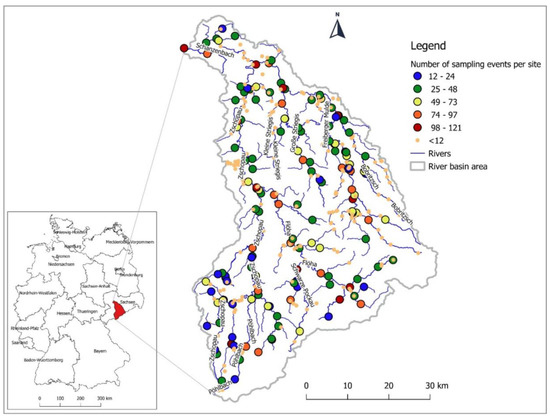
Figure 1.
Location map of the study area with number of sampling events per water quality monitoring (WQM) site during the monitoring period of 2006 to 2016 on the Freiberger Mulde river basin in eastern Germany.
2.2. Data Selection and Preparation
The monitoring data for the FM river basin, which have been collected by the Free State of Saxony since 1999 and which are freely accessible on their water quality database platform, were used for this research [32]. The process of preparing the dataset for the application of multivariate statistical analysis consisted of selecting water quality variables and monitoring stations, while minimizing the missing values. The water quality parameters that were considered for current analysis include chemical and physiochemical elements that explain the catchment processes, such as the influence of both the drainage basin and local environmental conditions. For this reason, long-term and frequently-monitored parameters were prioritized. Parameters with data availability of less than 30% or with censored data comprising more than 15% (concentrations below the detection limits and/or below the quantitation limits of the analytical methods) were excluded. The records under the censor limits were replaced by half of the detection limits and/or quantitation limits. According to the United States Environmental Protection Agency [33], this percentage of censored data is acceptable for a substitution method. The soluble concentrations in total water samples were used for the analysis. Maps of the river basin and monitoring stations were also obtained via Saxony’s open access on geodata portal [34].
The selection of monitoring stations was based on the availability of monitoring data. In this study, we considered the monitoring stations that had at least three years of monitoring data and 12 sampling events (Figure 1). The continuity of the monitoring years was not necessarily required, because the variables were assumed to be independent and identically distributed.
2.3. Principal Component Analysis
Principal component analysis (PCA) is a popular multivariate statistical technique used for dimension reduction [35]. PCA provides information on the most meaningful variables, thus describing the whole dataset and rendering data reduction with a minimum loss of the original information [1]. PCA transforms the original variables into new, uncorrelated variables called the principal components (PCs) [36]. The calculation to obtain PCs is given in Abdi and Williams [19]. In this study, PCA is implemented based on the correlation matrix. In instances where the variables are highly correlated, the first few principal components may be sufficient to describe most of the variability of the dataset [37]. The importance of a component is reflected by its eigenvalue. PCs with eigenvalues less than one are commonly recommended to be ignored [1,22,38]. To strengthen the interpretation, PCs with eigenvalues more than one are subjected to the varimax rotation, which generates rotated components (RCs). RCs further simplify the data structure coming from PCA [1,22]. The varimax rotation technique prevents multiple variables from being loaded to a single component, allowing for easy interpretation of significant variables [24]. Because these rotations are performed in a subspace, the new rotated components explain less variance than the original principal components, but the total variance remains the same after rotation [19].
In PCA, the correlations between a variable and a component are loadings, which estimate the information that they share. For interpretation, variables that have absolute values of loadings greater than or equal to 0.7 are strongly correlated, from 0.5 to 0.7 are moderately correlated, and less than 0.5 are weakly correlated to the component [1,22]. In other words, the larger the loading values, the more important that variable is to explain the component. The length of the projection of the observations on the components are factor scores. The importance of an observation for a component can be obtained by the ratio of the squared factor score of this observation to the sum of squared factor scores of all observations in the component [19]. This ratio is called contribution of the observation to the component. Details of the equations to calculate loadings, factor scores, and observation contributions can be found in Abdi and Williams [19]. For a given component, the sum of the contributions of all observations is equal to 1. Thus, the larger the value of the contribution, the more the observation contributes to explaining the component [19]. In this study, the observation contributions in percentage are used to calculate the importance of the monitoring sites in explaining the spatial variability and importance of the monitoring months in explaining temporal variability of the water quality. On each component, the contribution of a monitoring site is calculated as the sum of the contributions of all observations on that site during the whole monitoring period. Similarly, the contribution per monitoring month is calculated as the sum of contributions of all observations of all sites on that month. The variance explained by a monitoring site at any component is quantified by the product of its contribution and the variance explained by the selected component.
PCA is carried out in R software, and varimax rotation is implemented on R package psych [39]. The factor scores, loadings, and contribution of observation can be directly extracted using R package FactoMineR [40]. Map visualizations of PCA’s results are implemented on QGIS (version 2.18.16) software [41].
3. Results and Discussion
3.1. Data Screening and Descriptive Statistics
A thorough review of the existing dataset revealed that the timing of the sample collection was routine and not intended to capture any specific event. Of the monitoring sites of small tributaries, some were dismissed in 2006 and some were added after 2007. Only the main river and big tributaries such as Zschopau, Flöha, Gimlitz, Pockau, and Hüttenbach have been monitored long enough to obtain continuous data series from 1999 to 2016. This could be a result of the WFD implementation in Germany, where one of the WFD-mandated deadlines for “setting up networks and putting them into operation” was December 2006 [42]. For this reason, the monitoring period considered in this study is restricted to 2006–2016.
Although more than 80 water quality parameters were screened, only 23 parameters were selected based on the criteria mentioned in Section 2.2. After the initial screening, the selected database included 7541 sampling events covering 23 parameters at 151 monitoring sites, for a period of 11 years (2006 to 2016). A descriptive statistics summary with the percentages of censored data is presented in Table 1. The monitoring sites cover the large streams of Freiberger Mulde, Zschopau, Große Striegis, Flöha, Bobritzsch, Aschbach, and 75 other smaller tributaries. It is noted that most of the parameters do not follow normal distribution with high standard deviation and skewness, with the exceptions of oxygen and temperature (Table 1). For principal component analysis, non-normal data is log-transformed and then standardized to zero mean and unit of variance to avoid misclassification arising from different scales and units of the monitored variables.

Table 1.
Statistical summary of 23 analyzed water quality parameters in the Freiberger Mulde river basin from 2006 to 2016.
3.2. Characterized Water Quality Parameters and Sources Identification Based on Factor Loadings
The results of the principal component analysis for the data matrix of (7541 observations × 23 variables) in the FM river basin are shown in Table 2. There are five principal components (PCs) with the eigenvalue more than one, explaining 75.1% of the water quality variability (Figure 2). PC1 is strongly and positively correlated to HCO3−, Ca2+, Cl−, Mg2+, K+, Na+, SO42−, Boron and TIC and moderately correlated to NO3− and TON. The sources of these ionic concentrations may have multiple origins: rainfall, weathering of silicate and carbonate minerals, dissolved minerals contained in some sedimentary rocks, or leaching from the soil surface during rainstorms [43]. The first PC represents the weathering process and explains 37.6% of the total water quality variability in the river basin. The second component accounts for 12.9% of the observed data variability and has strong negative loadings on zinc and moderate loadings on nickel, fluoride, and arsenic. These trace metals and anions appear naturally in river waters through the weathering of minerals and also anthropogenically through the mixing of industrial effluents into the river streams and non-point pollution sources [44]. Taking into account the historical mining activities in the FM river basin [30], the major sources of PC2 are likely related to abandoned mines in the Ore Mountains. The third component explains 11.9% of the total variance and has negative strong loadings on dissolved organic carbon and total organic carbon and positive moderate loadings on turbidity and NO3−. PC3 represents organic matter, which could originate from the natural decomposition of organic material, as well as anthropogenic activities including agriculture and domestic wastewater discharges [45]. PC4 shows the inverse relationship between temperature and oxygen, representing the seasonal effects and explaining 7.4% of the variance. PC5 accounts for only 5.3% of the data variability and does not show strong or moderate correlation to any variable.
Table 2.
Loadings of the variables on the first five components according to PCA and varimax-rotated PCA.

Figure 2.
Eigenvalues and cumulative variance explained for 23 principal components from principal component analysis (PCA).
To strengthen the interpretation, varimax rotation was applied for the first five principal components and resulted in a new set of loadings (Table 2). For the first four components, PCA and varimax-rotated PCA gives the same interpretation of the hidden factors that affect the water quality variability of the FM river basin. The first rotated component (RC) links to the major ions and total inorganic carbon but only explains 34.9% instead of 37.6% of the data variability. RC2 also relates to mining activities and weathering processes, but with strong loadings on arsenic and fluoride and moderate loading on zinc, it explains only 11.2% of the total variance. RC3 conveys the same strong correlation to organic carbon and turbidity and accounts for 11.4% of the observed variability. RC4 shows the seasonal effects with strong positive loading on temperature and negative loading on oxygen, which explains 9% of the total variance. It is only on the fifth component that the varimax rotation shows a strong loading of manganese and moderate loadings of nickel and zinc and this explains 8.7% of the total variance. Therefore, the sources of RC5 could also be the weathering processes and the historic mining activities. In combining the results from PCA and varimax rotation, the major sources of surface water quality variation in FM river include weathering process, mining activities, agriculture, seasonality, and wastewater effluents. For the first five components, 75.1% of the variance can be explained by 18 parameters: HCO3−, Ca2+, Cl−, Mg2+, K+, Na+, SO42−, Boron, TIC, Arsenic, Zinc, Nickel, Fluoride, DOC, TOC, Temperature, Oxygen, and Manganese. Notably, PCA does not give a substantial data reduction with more than 78% of the parameters (18 out of 23) to explain 75.1% of the data variation.
PCA does not explicitly account for the redundancy of correlated variables. To further reduce the number of monitoring parameters, Pearson’s correlation coefficients for all 23 parameters were computed for the entire monitoring period (Figure 3). If the correlation coefficient is between 0.9 and 1 (or −0.9 and −1), the two variables are highly correlated and can be represented by a linear relationship. Thus, for the paired variables that have correlation coefficients of more than 0.9, one of them could be discarded to reduce the redundancy of the information, e.g., Cl− − Na+ (0.92), HCO3− − TIC (0.96), Ca2+ − Mg2+ (0.92), and DOC − TOC (0.94), with the variable of higher loading on the principal component being kept. Consequently, combining the PCA results and Pearson correlation analysis, four parameters (Na+, HCO3−, Mg2+, DOC) can be further discarded. As a result, 14 variables (Boron, Calcium, Chloride, Potassium, Sulphate, TIC, Fluoride, Arsenic, Zinc, Nickel, Temperature, Oxygen, TOC, and Manganese) now explain 75% of the total variance, and therefore, should remain under observation.
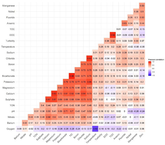
Figure 3.
Pearson correlation matrix of 23 parameters during the whole monitoring period. The numbers are correlation coefficients.
3.3. Spatial and Temporal Variability of Water Quality Based on the Contribution of Observations
Variation of water quality is captured and represented by sampling points (geographical or pollution effect) and sampling months (seasonal effect) [20]. In this study, the contributions of monitoring sites were used to visualize the spatial variation of water quality in the FM river basin (Figure 4). For a given component, the value of contributions in percentage are summed up to 100, with the variance explaining the monitoring sites summed up to the variance explained by that component. One percentage of contribution is recommended as the threshold to decide if a monitoring site is critical on a specific component. As such, 25 monitoring sites contribute more than one percent to PC1. They are located mostly on the upstream tributaries (16 sites) and partly on the FM river and its small first-order streams (9 sites). These monitoring sites make up 23% out of 37.6% of variance explained by the first component. The weathering process is therefore spatially dependent and plays an important role in the upstream and mainstream of the FM river basin in explaining the water quality variance. The second component shows higher contributions in three places: Wilisch (in the upper west of the river basin) and Roter Graben and Münzbach streams, which are close to Freiberg city where abandoned mines and heavy industries are located. On the contrary, monitoring sites where organic matter was observed showed that this component was homogenously distributed across the river basin, with only minor variations being observed. Notably, the highest contribution site to PC3 (10.1%) is located on Lampertsbach, which is a 5.6-km long stream running through the populated area of Cranzahl and connected to the Sehma river. The second-highest contribution site of organic matter was shown to be on the Schwarze Pockau, derived from bog-water in the Ore Mountains. Like PC3, the fourth component (PC4) was evenly distributed among the monitoring sites, with a maximum deposit of only 1.75% on Zschopau river, again showing that temperature and oxygen contribute to minor spatial variations. The most relevant sites for measuring the fifth component (PC5) are located on the Graben and Münzbach streams, with both being affected by mining discharges from Freiberg city industry.

Figure 4.
Spatial variation of the five major factors in explaining the data variability in Freiberger Mulde river basin based on the contribution of monitoring sites to (a) Principal component 1—weathering and leaching processes, (b) Principal component 2—industrial and mining impacts, (c) Principal component 3—organic matter, (d) Principal component 4—seasonality, (e) Principal component 5—weathering and mining impacts.
The temporal variability of each principal component was analyzed according to the monthly contributions of each observed component, and calculated using the total amount of observations. The contribution per component over a 12 months period was summed up to 100%; if each month shows an equal contribution, the period of time sampled shows a negligible impact on that component. A fluctuation in contributions over several months indicated that the component is subjected to temporal variation, with a higher contribution suggesting the influence of the time period. Figure 5 shows the contribution over the entire monitoring period of 12 months (January to December) for the first five components. The first component (PC1) remains almost constant over the 12 months, with a minor contribution shift observed during the cold season of November to March, potentially because the rate of chemical weathering decreases with the decreasing temperature [46]. This also indicates the minor influence of the sampling months on the mineral contents in the FM river basin. For the second component, a weak point is shown during warm periods, accompanied by a peculiar pattern of higher and lower contributions, differing from month to month, with low contributions in even months and high contributions in odd months. While the reason for this oscillating contribution remains unclear, the observations suggested that the monitoring schemes favored odd months over even months. The fluctuations in components three and four are quite similar: in PC3, the maximum variation of organic matter is observed in July (12.1%), which is almost twice the contribution of April (5.6%) and December (5.9%). The higher contribution of organic matter from June to September could be related to lower and more variable flow during summertime. In PC4, the extreme warm (July to September) and cold months (January to March) play a bigger role than the milder months of April, May, and October in demonstrating the variation. The fifth component resembles patterns of the first and second component, with less seasonal variation of manganese in the FM river basin.
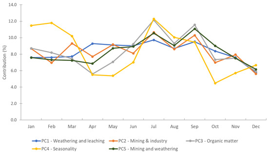
Figure 5.
Temporal variation of the five major factors in explaining the data variability in Freiberger Mulde river basin over the whole monitoring period of 2006 to 2016 based on the contribution of 12 monitoring months.
Based on the contributions of observations from PCA, the mineral contents (major ions) in the FM river basin are mainly impacted by sampling locations rather than seasonality. In contrast, sampling months play a more important role in explaining the variation of organic matter, temperature, and oxygen than sampling locations. Both monitoring schemes and locations influence the heavy metals variation in the FM river basin. Temporally, July and September contribute the most and December the least in explaining the data variability. As an implication, monitoring strategies should focus more on the warmer months to capture the most variability of water quality in the FM river basin. The significance of discharge variability for concentration variability should be further studied. Spatially, areas close to Freiberg city and to the upper west of the river basin are the hotspots in terms of heavy metals and mineral contents in explaining the water quality variations.
3.4. Cost-Effectiveness of Proposed Water Quality Monitoring Network Based on PCA Results
Although the principal component analysis helped to identify the critical factors, variables, and monitoring sites that explain the water quality variability, this information still does not constitute a criterion to decide if the proposed variables and sites present the optimum options. This section strives to provide a solution to this problem by quantifying the cost-effectiveness of the monitoring network based on the results from PCA. According to Harmancioglu, et al. [10], a possible way of measuring the benefits of monitoring practice can be the information conveyed by the collected data. This study was conducted under the assumption that the “effectiveness” or the “information” of a monitoring network corresponds to the water quality variance deriving from the monitoring data collected. The information is therefore equivalent to the variance explained by the principal components: specifically, if only strong loading parameters on the first component (Ca2+, Cl−, Mg2+, K+, Na+, SO42−, Boron, and TIC) are monitored for all monitoring sites, then only 37.6% of water quality variability is preserved. Cumulatively, if all 10 strong loading variables on PC1 and PC2 are monitored (at all 151 monitoring sites), then the monitoring network retains 50.5% of its information. Depending on the monitoring requirement, the water managers can select the parameters for observations on specific components accordingly.
Monitoring costs in the state of Saxony are program-based and the monitoring prices of different parameters are not available. Therefore, we estimated the monitoring costs based on the 2019 services’ price list of Brandenburg, another State in Germany that neighbors Saxony [47]. These estimations include the cost of transportation (for an average of 10 monitoring sites per day), sampling, and laboratory analysis. Detailed prices are given in Table 3. If only the laboratory cost was considered, monitoring of organic matter (PC3), temperature and oxygen (PC4), and inorganic contents (PC1) would be more economical compared to the heavy metals (PC2 and PC5), with the percentage of information achieved per euro being 0.71, 0.68, 0.58, and 0.19, respectively. Furthermore, monitoring of all 23 variables appeared to be less economical than monitoring the 14 critical variables of the first five components.
Table 3.
Price in euro for transportation, sampling, and laboratory analysis according to Brandenburg services price list in 2019.
Each monitoring site has a different contribution to a component to explain the total variance; the variance explained by a monitoring site i on j components, denoted , is calculated as:
where is the contribution of monitoring site i on component j, and is the variance explained by j-th component. The variance explained by monitoring sites on each component is given in Annex 1. According to the monitoring variables and number of monitoring sites, sampling and monitoring costs are estimated for one monitoring event. To quantify the cost at different levels of information achieved, the monitoring costs were estimated for five scenarios:
- PC1: monitoring of six variables strongly correlated to PC1 (Ca2+, Cl−, K+, SO42−, Boron, and TIC) and obtaining 37.6% of information accordingly;
- PC1,2: monitoring of 10 variables strongly correlated to PC1 and PC2 (Ca2+, Cl−, K+, SO42−, Boron, TIC, Fluoride, Arsenic, Zinc, Nickel) and obtaining 50.5% of information accordingly;
- PC1,3,4: monitoring of nine variables strongly correlated to PC1, PC3, and PC4 (Ca2+, Cl−, K+, SO42−, Boron, TIC, TOC, temperature, oxygen) and obtaining 56.9% of information accordingly;
- PC1-5: monitoring of 14 variables correlated to the first five components (Ca2+, Cl−, K+, SO42−, Boron, TIC, Fluoride, Arsenic, Zinc, Nickel, TOC, Oxygen, Temperature, Manganese) and obtaining 75.1% of information accordingly; and
- All PC: monitoring of all 23 variables and obtaining 100% of the information.
An adaptation from the cost-effectiveness plane illustrating the information and the costs of different monitoring options is shown in Figure 6. Monitoring sites are in descending order based on their contributions to the variance explained (given in Appendix A) for calculating cumulative variance. The cost-effectiveness plane in our case consists of four-quadrants: high information—low cost, high information—high cost, low information—high cost, and low information—low cost. Five strategies of variable selection according to the variance explained by principal components are also displayed in the same diagram (Figure 6). The current monitoring practice of 23 variables at 151 monitoring sites would give 100% of information on data variability at estimated 51,507 euro per monitoring event (equivalent to 100% cost). A reduction of monitoring sites or WQ variables would result in a decrease in the information achieved as well as the monitoring costs. As such, monitoring of six variables of PC1 (Ca2+, Cl−, K+, SO42−, Boron, and TIC) at 151 sites would cost 17,487 euro (40% of the total cost) but would only give 37.6% of the information. Monitoring the 10 variables of PC1 and PC2 (Ca2+, Cl−, K+, SO42−, Boron, TIC, Fluoride, Arsenic, Zinc, Nickel) at 151 sites would explain 50.5% of the information at the cost of 26,411 euro (~51.2% compared to the total cost). The PC1 curve lies completely in the low information—low cost quadrant, while the PC1,2 curve exceeded 50% of the cost at 148 sites. Combination of three components (PC1,3, and 4) with cost-effective variables explained 57% of the data variability at the cost of 21,669 euro for all sites, which provides more information at less cost than the combination of PC1 and 2. The high laboratory costs of heavy metals made the cost of PC1,2 curve increase faster than the information added, as compared to the PC1 and PC1,3,4 curves. Although the curves of PC1-5 and All PC expand in three quadrants, it is deemed more effective to monitor more variables at fewer sites than the opposite practice. For example, to achieve 75.1% of information, measuring 14 variables at 151 sites would cost 34,837 euro while monitoring all variables at 72 sites provides the same amount of information and would only cost 24,616 euro. It is noteworthy that the strategies all parameters (All PC), main parameters (PC1-5), and cost-effective parameters (PC1,3,4) perform similarly: up to 45% information, although they differ in their emphasis on number of sites versus number of parameters. Other options with different level of cost and information achieved can be compared easily using the rank of monitoring sites in Annex 1 and price list in Table 3.

Figure 6.
The cost-information plane for different monitoring strategies. PC1 (37.6%)—monitoring 6 water quality variables at one to 151 sites, PC1,2 (50.5%)—monitoring 10 variables at one to 151 sites, PC1,3,4—monitoring 9 variables at one to 151 sites, PC1-5 (75.1%)—monitoring 14 variables at one to 151 sites, and All PC (100%)—monitoring 23 variables at one to 151 sites.
The most challenging aspect of this approach is the selection of the representative variables on the principal components. In this study, strong loading variables (loadings > 0.7) with low correlation coefficient (<0.9) were selected; by ignoring other variables, part of the variance explained would certainly be lost. In addition, the input for PCA requires no missing data; thus, this approach is data-dependent and only applicable when a decision must be made to remove monitoring sites or WQ parameters. The quantification of information based on the variance explained limits the objective of the designed monitoring network to the determination of changes in water quality only, without consideration of other specific objectives such as trend detection and compliance monitoring. Finally, the cost estimation was simplified for one monitoring event without consideration of other fixed and operational costs of a monitoring program. In order to curb these limitations and provide a more effective monitoring network design, future research should consider the quantification of multi-objectives monitoring network (data quality, information accuracy, statistical methods, monitoring costs, stakeholder views, social factors, etc.) and monitoring frequencies.
4. Conclusions
This study demonstrates the usefulness of principal component analysis (PCA) in analyzing the complex dataset to address the water quality management in rivers. PCA proves to be useful for the analysis of 11-year irregular monitoring data from the Freiberger Mulde (FM) river basin, which is comprised of 23 water quality parameters and 151 monitoring sites. A combination of PCA and Pearson’s correlation analysis allowed for identification of 14 critical parameters that are responsible for explaining 75.1% of data variability in the river basin. Weathering processes, historical mining, wastewater discharges, and seasonality are the main causes of the river water quality variability. The contributions calculated from factor scores are very insightful in interpreting spatial and temporal sources of water quality variations. As such, heavy metals are impacted by both sampling locations and sampling time. Specifically, Wilisch (in the upper west of the river basin), Roter Graben, and Münzbach streams, which are close to the Freiberg city, appear to be the best selections for monitoring of heavy metals. Monitoring of those significant sites is recommended to guarantee the continuity of effective water quality monitoring in the future. The mineral contents play an important role in explaining the water quality variations of the FM river basin and are impacted more by the sampling locations than the sampling months. The variation of organic matter, oxygen, and temperature, in contrast, are more dependent on the sampling months rather than the sampling locations, with July and September contributing to the highest variability in water quality. Temporarily, five major factors explaining water quality of the FM river basin vary the most in July and September and the least in December, hence the future monitoring scheme should concentrate more on the warmer months.
This work establishes a simple quantification of the cost-effectiveness framework of the monitoring networks based on PCA results for the FM river basin. Under the current monitoring-intense conditions, preserving monitoring variables rather than sites seems to be more economical than the opposite practice. To achieve 75% of variance, it is recommended to monitor 23 parameters at 72 monitoring sites, rather than monitoring 14 parameters at 151 monitoring sites, with the first option resulting in a cost decrease of 20% compared to the second option. Different variable selection strategies increase in significance depending on the requirement for substantial cost reductions. Up to 40% of information can be retained for less than 15% of current costs, at either 21 sites with all variables or 31 sites with the main variables (PCs 1-5), or 50 sites with more economical variables (PCs 1,3, and 4). This approach is restricted to quantify the basin-wide variability of water quality based on the previously established water quality variables and sampling sites. Further quantification of monitoring frequencies still needs to be specified in order to assess the effectiveness of the monitoring network. Often, monitoring intends to assess the state or development of a water body. Objectives such as trend detection or compliance assessment require other evaluation criteria, rather than information explained. The monitoring costs in this study were estimated only based on laboratory, transportation, and sampling costs, but the costs of the whole monitoring program can be easily incorporated into the presented approach if the data of monitoring period, frequencies, and other costs (logistics, personnel, maintenances, etc.) are available. This approach may support water managers and practitioners in selecting the optimum monitoring sites and variables through a rational understanding of the dynamic sources of water quality, when there is a need to reduce the monitoring costs.
Author Contributions
Conceptualization: T.H.N., B.H.; data analysis: T.H.N.; writing and first draft preparation: T.H.N.; reviewing: B.H., H.H., S.C.; research supervision: H.H., P.K. All authors have read and agreed to the published version of the manuscript.
Funding
This study is funded by German Academic Exchange Service (DAAD) and The United Nations University Institute for Integrated Management of Material Fluxes and of Resources (UNU-FLORES). Open Access Funding by the Publication Fund of the TU Dresden
Acknowledgments
We would like to thank our colleagues Stacy Roden, Louisa Andrews, and Mahesh Jampani for proofreading this manuscript. We further esteem the open data policy of Saxon State Office for the Environment, Agriculture and Geology as well as the provision of monitoring costs by Berlin-Brandenburg state laboratory.
Conflicts of Interest
The authors declare no conflicts of interest.
Appendix A
Table A1.
The variance (in percentage) explained by each monitoring site on selected principal components.
Table A1.
The variance (in percentage) explained by each monitoring site on selected principal components.
| Site | River | PC1 | PC2 | PC3 | PC4 | PC5 | PC1,2 | PC1,3,4 | PC1-5 | All PCs |
|---|---|---|---|---|---|---|---|---|---|---|
| OBF31301 | Freiberger Mulde | 0.206 | 0.015 | 0.125 | 0.092 | 0.059 | 0.222 | 0.424 | 0.498 | 0.689 |
| OBF31302 | Zethaubach | 0.066 | 0.037 | 0.054 | 0.032 | 0.004 | 0.102 | 0.151 | 0.192 | 0.283 |
| OBF31303 | Helbigsdorfer Bach | 0.032 | 0.078 | 0.037 | 0.048 | 0.009 | 0.110 | 0.117 | 0.205 | 0.296 |
| OBF31400 | Freiberger Mulde | 0.081 | 0.041 | 0.076 | 0.043 | 0.036 | 0.122 | 0.200 | 0.277 | 0.422 |
| OBF31500 | Freiberger Mulde | 0.094 | 0.011 | 0.053 | 0.036 | 0.040 | 0.105 | 0.183 | 0.234 | 0.573 |
| OBF31510 | Freiberger Mulde | 0.156 | 0.059 | 0.052 | 0.030 | 0.046 | 0.215 | 0.238 | 0.343 | 0.650 |
| OBF31520 | Freiberger Mulde | 0.042 | 0.039 | 0.012 | 0.009 | 0.010 | 0.081 | 0.063 | 0.112 | 0.182 |
| OBF31530 | Stangenbergbach | 0.075 | 0.220 | 0.042 | 0.012 | 0.045 | 0.295 | 0.130 | 0.395 | 0.544 |
| OBF31540 | Hüttenbach | 0.312 | 0.069 | 0.071 | 0.032 | 0.038 | 0.381 | 0.415 | 0.522 | 0.793 |
| OBF31600 | Freiberger Mulde | 0.181 | 0.198 | 0.037 | 0.040 | 0.027 | 0.379 | 0.258 | 0.483 | 0.806 |
| OBF31601 | Kleinwaltersdorfer Bach | 0.020 | 0.011 | 0.023 | 0.056 | 0.010 | 0.031 | 0.100 | 0.121 | 0.213 |
| OBF31610 | Freiberger Mulde | 0.212 | 0.073 | 0.019 | 0.023 | 0.035 | 0.285 | 0.255 | 0.362 | 0.429 |
| OBF31700 | Freiberger Mulde | 0.739 | 0.255 | 0.070 | 0.070 | 0.112 | 0.994 | 0.880 | 1.246 | 1.510 |
| OBF31701 | Freiberger Mulde | 0.178 | 0.049 | 0.017 | 0.008 | 0.028 | 0.227 | 0.204 | 0.281 | 0.333 |
| OBF31710 | Freiberger Mulde | 0.215 | 0.039 | 0.028 | 0.017 | 0.029 | 0.253 | 0.260 | 0.328 | 0.395 |
| OBF31711 | Pitzschebach | 0.151 | 0.013 | 0.057 | 0.089 | 0.118 | 0.164 | 0.298 | 0.428 | 0.686 |
| OBF31800 | Freiberger Mulde | 0.189 | 0.035 | 0.021 | 0.024 | 0.023 | 0.224 | 0.233 | 0.291 | 0.346 |
| OBF31801 | Marienbach | 0.178 | 0.035 | 0.043 | 0.045 | 0.041 | 0.212 | 0.266 | 0.342 | 0.442 |
| OBF31900 | Freiberger Mulde | 0.195 | 0.034 | 0.022 | 0.024 | 0.022 | 0.229 | 0.241 | 0.297 | 0.358 |
| OBF31950 | Freiberger Mulde | 0.182 | 0.029 | 0.029 | 0.031 | 0.015 | 0.211 | 0.241 | 0.285 | 0.357 |
| OBF32000 | Freiberger Mulde | 0.462 | 0.065 | 0.070 | 0.076 | 0.038 | 0.527 | 0.608 | 0.711 | 0.859 |
| OBF32001 | Gärtitzer Bach | 0.598 | 0.083 | 0.043 | 0.074 | 0.063 | 0.682 | 0.715 | 0.862 | 1.005 |
| OBF32201 | Görnitzbach | 0.790 | 0.247 | 0.170 | 0.086 | 0.059 | 1.036 | 1.046 | 1.351 | 1.571 |
| OBF32202 | Schickelsbach | 0.347 | 0.062 | 0.075 | 0.036 | 0.042 | 0.409 | 0.458 | 0.562 | 0.690 |
| OBF32203 | Polkenbach | 0.559 | 0.143 | 0.050 | 0.063 | 0.045 | 0.702 | 0.672 | 0.860 | 0.991 |
| OBF32204 | Polkenbach | 0.334 | 0.055 | 0.019 | 0.047 | 0.052 | 0.389 | 0.399 | 0.507 | 0.598 |
| OBF32205 | Fritzschenbach | 0.365 | 0.064 | 0.073 | 0.072 | 0.070 | 0.429 | 0.511 | 0.645 | 0.778 |
| OBF32206 | Schanzenbach | 0.493 | 0.232 | 0.217 | 0.088 | 0.086 | 0.726 | 0.798 | 1.117 | 1.299 |
| OBF32300 | Freiberger Mulde | 0.251 | 0.032 | 0.092 | 0.092 | 0.057 | 0.282 | 0.434 | 0.523 | 0.742 |
| OBF32600 | Chemnitzbach | 0.079 | 0.035 | 0.115 | 0.044 | 0.022 | 0.114 | 0.237 | 0.294 | 0.406 |
| OBF32601 | Voigtsdorfer Bach | 0.087 | 0.005 | 0.063 | 0.026 | 0.008 | 0.092 | 0.176 | 0.189 | 0.342 |
| OBF32700 | Grosshartmannsdorfer Bach | 0.064 | 0.110 | 0.096 | 0.081 | 0.011 | 0.175 | 0.242 | 0.363 | 0.568 |
| OBF32750 | Gimmlitz | 0.293 | 0.027 | 0.116 | 0.067 | 0.008 | 0.320 | 0.476 | 0.511 | 0.657 |
| OBF32800 | Gimmlitz | 0.100 | 0.048 | 0.105 | 0.043 | 0.015 | 0.148 | 0.249 | 0.312 | 0.452 |
| OBF32900 | Münzbach | 2.102 | 0.153 | 0.243 | 0.089 | 0.206 | 2.255 | 2.434 | 2.793 | 3.363 |
| OBF32901 | Münzbach | 0.223 | 0.391 | 0.157 | 0.063 | 0.045 | 0.613 | 0.442 | 0.878 | 1.398 |
| OBF32903 | Münzbach | 0.349 | 0.050 | 0.039 | 0.024 | 0.038 | 0.399 | 0.413 | 0.501 | 0.728 |
| OBF33010 | Roter Graben | 0.157 | 1.909 | 0.055 | 0.054 | 0.675 | 2.066 | 0.266 | 2.849 | 3.273 |
| OBF33020 | Roter Graben | 0.414 | 1.154 | 0.035 | 0.054 | 0.425 | 1.568 | 0.504 | 2.082 | 2.405 |
| OBF33090 | Bobritzsch | 0.033 | 0.003 | 0.245 | 0.103 | 0.017 | 0.036 | 0.381 | 0.401 | 0.699 |
| OBF33100 | Bobritzsch | 0.018 | 0.048 | 0.086 | 0.060 | 0.073 | 0.066 | 0.164 | 0.285 | 0.515 |
| OBF33111 | Dittmannsdorfer Bach | 0.180 | 0.040 | 0.066 | 0.046 | 0.005 | 0.219 | 0.291 | 0.336 | 0.465 |
| OBF33200 | Bobritzsch | 0.051 | 0.061 | 0.100 | 0.106 | 0.100 | 0.112 | 0.257 | 0.418 | 0.657 |
| OBF33300 | Sohrbach | 0.018 | 0.018 | 0.042 | 0.042 | 0.015 | 0.036 | 0.101 | 0.134 | 0.455 |
| OBF33400 | Colmnitzbach | 0.023 | 0.017 | 0.033 | 0.048 | 0.020 | 0.040 | 0.105 | 0.142 | 0.234 |
| OBF33500 | Rodelandbach | 0.039 | 0.015 | 0.071 | 0.061 | 0.007 | 0.054 | 0.170 | 0.193 | 0.319 |
| OBF33601 | Erbisdorfer Wasser | 0.046 | 0.063 | 0.058 | 0.035 | 0.007 | 0.109 | 0.139 | 0.210 | 0.350 |
| OBF33650 | Grosse Striegis | 0.007 | 0.064 | 0.052 | 0.005 | 0.093 | 0.071 | 0.065 | 0.222 | 0.296 |
| OBF33701 | Oberreichenbacher Bach | 0.025 | 0.031 | 0.059 | 0.043 | 0.019 | 0.055 | 0.126 | 0.176 | 0.255 |
| OBF33702 | Schirmbach | 0.007 | 0.011 | 0.030 | 0.046 | 0.005 | 0.018 | 0.083 | 0.099 | 0.207 |
| OBF33703 | Kemnitzbach | 0.014 | 0.024 | 0.120 | 0.056 | 0.011 | 0.038 | 0.190 | 0.225 | 0.406 |
| OBF33710 | Grosse Striegis | 0.041 | 0.009 | 0.032 | 0.035 | 0.005 | 0.051 | 0.108 | 0.123 | 0.254 |
| OBF33711 | Langhennersdorfer Bach | 0.057 | 0.037 | 0.045 | 0.034 | 0.007 | 0.094 | 0.136 | 0.181 | 0.243 |
| OBF33713 | Aschbach | 0.058 | 0.029 | 0.027 | 0.068 | 0.037 | 0.088 | 0.154 | 0.220 | 0.468 |
| OBF33800 | Grosse Striegis | 0.096 | 0.012 | 0.061 | 0.066 | 0.008 | 0.108 | 0.223 | 0.243 | 0.422 |
| OBF33900 | Grosse Striegis | 0.249 | 0.027 | 0.085 | 0.093 | 0.010 | 0.276 | 0.427 | 0.464 | 0.676 |
| OBF34101 | Pahlbach | 0.043 | 0.025 | 0.037 | 0.035 | 0.028 | 0.069 | 0.116 | 0.169 | 0.287 |
| OBF34200 | Kleine Striegis | 0.178 | 0.054 | 0.034 | 0.056 | 0.006 | 0.232 | 0.267 | 0.328 | 0.425 |
| OBF34300 | Klatschbach | 0.506 | 0.104 | 0.085 | 0.107 | 0.015 | 0.611 | 0.698 | 0.818 | 1.219 |
| OBF34390 | Geyerbach | 0.271 | 0.340 | 0.006 | 0.006 | 0.050 | 0.611 | 0.283 | 0.673 | 0.831 |
| OBF34400 | Zschopau | 1.173 | 0.049 | 0.097 | 0.022 | 0.023 | 1.222 | 1.292 | 1.364 | 1.553 |
| OBF34401 | Geyerbach | 0.158 | 0.338 | 0.057 | 0.058 | 0.013 | 0.496 | 0.273 | 0.625 | 0.719 |
| OBF34403 | Greifenbach | 0.271 | 0.165 | 0.052 | 0.083 | 0.012 | 0.437 | 0.407 | 0.584 | 0.699 |
| OBF34404 | Greifenbach | 1.937 | 0.322 | 0.326 | 0.021 | 0.039 | 2.258 | 2.283 | 2.644 | 3.170 |
| OBF34405 | Zschopau | 0.203 | 0.015 | 0.028 | 0.008 | 0.009 | 0.218 | 0.239 | 0.262 | 0.352 |
| OBF34409 | Zschopau | 0.043 | 0.038 | 0.043 | 0.030 | 0.013 | 0.081 | 0.117 | 0.167 | 0.260 |
| OBF34601 | Hüttenbach | 0.124 | 0.046 | 0.112 | 0.107 | 0.103 | 0.170 | 0.343 | 0.492 | 0.690 |
| OBF34700 | Zschopau | 0.016 | 0.013 | 0.026 | 0.022 | 0.011 | 0.029 | 0.064 | 0.088 | 0.135 |
| OBF34701 | Venusberger Dorfbach | 0.056 | 0.010 | 0.067 | 0.032 | 0.005 | 0.066 | 0.155 | 0.171 | 0.282 |
| OBF34710 | Zschopau | 0.006 | 0.007 | 0.016 | 0.014 | 0.009 | 0.013 | 0.036 | 0.053 | 0.079 |
| OBF34801 | Dittmannsdorfer Bach | 0.009 | 0.014 | 0.052 | 0.027 | 0.005 | 0.023 | 0.089 | 0.108 | 0.183 |
| OBF34802 | Schwarzbach | 0.010 | 0.010 | 0.085 | 0.028 | 0.040 | 0.021 | 0.124 | 0.174 | 0.272 |
| OBF34890 | Zschopau | 0.013 | 0.010 | 0.029 | 0.035 | 0.016 | 0.023 | 0.077 | 0.103 | 0.155 |
| OBF34900 | Zschopau | 0.024 | 0.025 | 0.058 | 0.050 | 0.022 | 0.049 | 0.132 | 0.179 | 0.287 |
| OBF34901 | Eubaer Bach | 0.382 | 0.020 | 0.052 | 0.046 | 0.007 | 0.403 | 0.479 | 0.507 | 0.673 |
| OBF34910 | Zschopau | 0.026 | 0.019 | 0.053 | 0.072 | 0.035 | 0.045 | 0.151 | 0.206 | 0.321 |
| OBF35001 | Mühlbach | 0.016 | 0.020 | 0.051 | 0.026 | 0.032 | 0.036 | 0.093 | 0.145 | 0.231 |
| OBF35002 | Lützelbach | 0.181 | 0.017 | 0.019 | 0.040 | 0.008 | 0.199 | 0.240 | 0.266 | 0.365 |
| OBF35003 | Holzbach | 0.132 | 0.013 | 0.036 | 0.034 | 0.013 | 0.146 | 0.203 | 0.229 | 0.308 |
| OBF35101 | Ottendorfer Bach | 0.097 | 0.028 | 0.038 | 0.046 | 0.011 | 0.125 | 0.181 | 0.220 | 0.306 |
| OBF35102 | Altmittweidaer Bach | 0.339 | 0.050 | 0.061 | 0.076 | 0.011 | 0.390 | 0.476 | 0.538 | 0.685 |
| OBF35103 | Auenbach | 0.103 | 0.048 | 0.036 | 0.041 | 0.010 | 0.151 | 0.180 | 0.239 | 0.320 |
| OBF35200 | Zschopau | 0.041 | 0.020 | 0.090 | 0.078 | 0.024 | 0.061 | 0.209 | 0.252 | 0.390 |
| OBF35251 | Schweikershainer Bach | 0.151 | 0.059 | 0.054 | 0.063 | 0.016 | 0.210 | 0.267 | 0.343 | 0.445 |
| OBF35252 | Richzenhainer Bach | 0.324 | 0.092 | 0.069 | 0.066 | 0.012 | 0.416 | 0.459 | 0.564 | 0.736 |
| OBF35253 | Richzenhainer Bach | 0.595 | 0.034 | 0.055 | 0.073 | 0.056 | 0.629 | 0.723 | 0.813 | 0.998 |
| OBF35254 | Gebersbach | 0.340 | 0.084 | 0.089 | 0.069 | 0.051 | 0.425 | 0.498 | 0.634 | 0.834 |
| OBF35255 | Eulitzbach | 0.374 | 0.059 | 0.137 | 0.089 | 0.094 | 0.433 | 0.599 | 0.752 | 1.012 |
| OBF35257 | Mortelbach | 0.222 | 0.072 | 0.028 | 0.030 | 0.006 | 0.294 | 0.280 | 0.358 | 0.456 |
| OBF35258 | Mortelbach | 0.182 | 0.027 | 0.055 | 0.096 | 0.048 | 0.209 | 0.333 | 0.408 | 0.688 |
| OBF35310 | Zschopau | 0.008 | 0.004 | 0.017 | 0.010 | 0.005 | 0.012 | 0.035 | 0.044 | 0.070 |
| OBF35350 | Zschopau | 0.075 | 0.063 | 0.137 | 0.130 | 0.042 | 0.138 | 0.341 | 0.447 | 0.683 |
| OBF35391 | Rote Pfütze | 0.007 | 0.119 | 0.025 | 0.016 | 0.149 | 0.126 | 0.047 | 0.315 | 0.445 |
| OBF35400 | Rote Pfütze | 0.110 | 0.009 | 0.077 | 0.041 | 0.008 | 0.119 | 0.228 | 0.245 | 0.358 |
| OBF35490 | Sehma | 1.355 | 0.013 | 0.088 | 0.057 | 0.020 | 1.368 | 1.500 | 1.533 | 1.736 |
| OBF35600 | Sehma | 0.100 | 0.024 | 0.025 | 0.019 | 0.003 | 0.124 | 0.143 | 0.171 | 0.223 |
| OBF35601 | Lampertsbach | 1.127 | 0.320 | 1.209 | 0.117 | 0.019 | 1.446 | 2.453 | 2.791 | 3.774 |
| OBF35602 | Lampertsbach | 0.119 | 0.007 | 0.007 | 0.009 | 0.003 | 0.125 | 0.135 | 0.145 | 0.216 |
| OBF35650 | Sehma | 0.046 | 0.020 | 0.014 | 0.007 | 0.003 | 0.066 | 0.067 | 0.090 | 0.142 |
| OBF35800 | Sehma | 0.070 | 0.036 | 0.056 | 0.064 | 0.053 | 0.106 | 0.190 | 0.279 | 0.572 |
| OBF35802 | Sehma | 0.102 | 0.193 | 0.023 | 0.077 | 0.003 | 0.295 | 0.201 | 0.397 | 0.565 |
| OBF36000 | Pöhlbach | 0.051 | 0.023 | 0.035 | 0.014 | 0.007 | 0.074 | 0.101 | 0.130 | 0.289 |
| OBF36100 | Pöhlbach | 0.031 | 0.007 | 0.021 | 0.014 | 0.009 | 0.038 | 0.066 | 0.081 | 0.207 |
| OBF36200 | Pöhlbach | 0.037 | 0.019 | 0.055 | 0.055 | 0.008 | 0.056 | 0.147 | 0.173 | 0.442 |
| OBF36300 | Pöhlbach | 0.026 | 0.012 | 0.058 | 0.035 | 0.007 | 0.038 | 0.119 | 0.138 | 0.266 |
| OBF36400 | Pressnitz | 1.101 | 0.015 | 0.078 | 0.031 | 0.048 | 1.116 | 1.210 | 1.274 | 1.572 |
| OBF36402 | Steinbach | 0.262 | 0.024 | 0.036 | 0.038 | 0.013 | 0.285 | 0.335 | 0.372 | 0.494 |
| OBF36403 | Haselbach | 0.384 | 0.011 | 0.024 | 0.028 | 0.004 | 0.394 | 0.436 | 0.450 | 0.629 |
| OBF36404 | Sandbach | 0.015 | 0.019 | 0.040 | 0.021 | 0.010 | 0.033 | 0.076 | 0.104 | 0.200 |
| OBF36450 | Pressnitz | 0.122 | 0.004 | 0.018 | 0.012 | 0.002 | 0.126 | 0.151 | 0.158 | 0.189 |
| OBF36500 | Pressnitz | 0.292 | 0.022 | 0.075 | 0.056 | 0.014 | 0.314 | 0.423 | 0.458 | 0.598 |
| OBF36600 | Jöhstädter Schwarzwasser | 0.553 | 0.023 | 0.047 | 0.039 | 0.015 | 0.575 | 0.639 | 0.677 | 0.952 |
| OBF36601 | Jöhstädter Schwarzwasser | 0.230 | 0.014 | 0.028 | 0.031 | 0.004 | 0.243 | 0.288 | 0.306 | 0.396 |
| OBF36700 | Rauschenbach | 0.118 | 0.029 | 0.079 | 0.028 | 0.014 | 0.147 | 0.225 | 0.268 | 0.435 |
| OBF36793 | Wilisch | 0.036 | 0.091 | 0.085 | 0.057 | 0.046 | 0.126 | 0.178 | 0.315 | 0.444 |
| OBF36794 | Wilisch | 0.131 | 0.874 | 0.032 | 0.060 | 0.010 | 1.004 | 0.224 | 1.107 | 1.469 |
| OBF36795 | Wilisch | 0.029 | 0.287 | 0.022 | 0.029 | 0.006 | 0.316 | 0.079 | 0.372 | 0.520 |
| OBF36797 | Wilisch | 0.015 | 0.062 | 0.048 | 0.031 | 0.017 | 0.077 | 0.094 | 0.173 | 0.238 |
| OBF36800 | Wilisch | 0.065 | 0.116 | 0.051 | 0.110 | 0.060 | 0.182 | 0.227 | 0.404 | 0.714 |
| OBF36801 | Jahnsbach | 0.022 | 0.017 | 0.066 | 0.040 | 0.006 | 0.039 | 0.127 | 0.151 | 0.259 |
| OBF36803 | Jahnsbach | 0.271 | 0.192 | 0.015 | 0.062 | 0.005 | 0.463 | 0.349 | 0.546 | 0.647 |
| OBF36850 | Flöha | 0.787 | 0.024 | 0.034 | 0.022 | 0.006 | 0.811 | 0.843 | 0.873 | 0.997 |
| OBF36911 | Cämmerswalder Dorfbach | 0.120 | 0.031 | 0.089 | 0.028 | 0.006 | 0.151 | 0.236 | 0.274 | 0.378 |
| OBF36912 | Mortelbach | 0.098 | 0.031 | 0.073 | 0.032 | 0.006 | 0.129 | 0.203 | 0.241 | 0.355 |
| OBF37000 | Flöha | 0.446 | 0.033 | 0.101 | 0.065 | 0.018 | 0.479 | 0.612 | 0.663 | 0.801 |
| OBF37001 | Rungstockbach | 0.509 | 0.009 | 0.023 | 0.028 | 0.021 | 0.518 | 0.560 | 0.590 | 0.721 |
| OBF37010 | Flöha | 0.236 | 0.015 | 0.057 | 0.049 | 0.011 | 0.251 | 0.342 | 0.368 | 0.499 |
| OBF37101 | Saidenbach | 0.064 | 0.055 | 0.026 | 0.022 | 0.018 | 0.120 | 0.112 | 0.185 | 0.266 |
| OBF37103 | Saidenbach | 0.064 | 0.079 | 0.058 | 0.046 | 0.020 | 0.143 | 0.168 | 0.267 | 0.359 |
| OBF37104 | Haselbach | 0.167 | 0.076 | 0.064 | 0.038 | 0.019 | 0.243 | 0.269 | 0.364 | 0.475 |
| OBF37105 | Lautenbach | 0.288 | 0.054 | 0.056 | 0.060 | 0.079 | 0.342 | 0.404 | 0.538 | 0.691 |
| OBF37106 | Röthenbach | 0.118 | 0.043 | 0.057 | 0.054 | 0.015 | 0.161 | 0.229 | 0.287 | 0.371 |
| OBF37300 | Flöha | 0.097 | 0.035 | 0.142 | 0.080 | 0.018 | 0.131 | 0.318 | 0.371 | 0.544 |
| OBF37400 | Schweinitz | 0.479 | 0.025 | 0.220 | 0.074 | 0.012 | 0.504 | 0.773 | 0.810 | 0.990 |
| OBF37401 | Seiffener Bach | 0.023 | 0.013 | 0.030 | 0.074 | 0.061 | 0.037 | 0.127 | 0.201 | 0.325 |
| OBF37404 | Seiffener Bach | 0.006 | 0.033 | 0.066 | 0.125 | 0.008 | 0.038 | 0.197 | 0.237 | 0.353 |
| OBF37450 | Natzschung | 0.300 | 0.003 | 0.030 | 0.013 | 0.002 | 0.303 | 0.343 | 0.349 | 0.390 |
| OBF37500 | Natzschung | 1.465 | 0.024 | 0.178 | 0.079 | 0.010 | 1.489 | 1.722 | 1.756 | 1.970 |
| OBF37600 | Bielabach | 0.039 | 0.049 | 0.043 | 0.025 | 0.009 | 0.089 | 0.107 | 0.165 | 0.251 |
| OBF37800 | Schwarze Pockau | 0.908 | 0.012 | 0.351 | 0.051 | 0.007 | 0.919 | 1.310 | 1.328 | 1.503 |
| OBF37910 | Schwarze Pockau | 1.196 | 0.022 | 0.423 | 0.089 | 0.009 | 1.219 | 1.708 | 1.740 | 1.976 |
| OBF38000 | Schwarze Pockau | 0.149 | 0.063 | 0.220 | 0.071 | 0.052 | 0.212 | 0.440 | 0.555 | 0.725 |
| OBF38100 | Rote Pockau | 0.024 | 0.033 | 0.084 | 0.025 | 0.046 | 0.057 | 0.133 | 0.212 | 0.300 |
| OBF38101 | Rote Pockau | 0.058 | 0.179 | 0.032 | 0.026 | 0.001 | 0.237 | 0.115 | 0.295 | 0.337 |
| OBF38190 | Rote Pockau | 0.001 | 0.118 | 0.013 | 0.032 | 0.006 | 0.118 | 0.046 | 0.170 | 0.210 |
| OBF38200 | Rote Pockau | 1.732 | 0.025 | 0.436 | 0.050 | 0.017 | 1.757 | 2.219 | 2.260 | 2.695 |
| OBF38201 | Schlettenbach | 0.088 | 0.015 | 0.020 | 0.034 | 0.034 | 0.103 | 0.143 | 0.192 | 0.305 |
| OBF38400 | Grosse Lössnitz | 0.019 | 0.080 | 0.097 | 0.052 | 0.019 | 0.099 | 0.168 | 0.266 | 0.477 |
| OBF38401 | Gahlenzer Bach | 0.025 | 0.027 | 0.049 | 0.045 | 0.022 | 0.052 | 0.120 | 0.169 | 0.304 |
| OBF38402 | Weissbach | 0.058 | 0.049 | 0.055 | 0.040 | 0.073 | 0.106 | 0.153 | 0.274 | 0.469 |
| OBF38500 | Hetzbach | 0.037 | 0.044 | 0.136 | 0.068 | 0.034 | 0.082 | 0.242 | 0.320 | 0.504 |
| Total variance explained (%) | 37.6 | 12.9 | 11.9 | 7.4 | 5.3 | 50.5 | 56.9 | 75.1 | 100 | |
Values in bold show the important sites on the principal components. PC3-organic matter and PC4-seasonality show a minor dependence on the sampling locations with the variance distributed quite homogenously among the sites. On the first five components, contribution of a monitoring site can be calculated as the quotient of its variance and the total variance explained by the component.
References
- Singh:, K.P.; Malik, A.; Mohan, D.; Sinha, S. Multivariate statistical techniques for the evaluation of spatial and temporal variations in water quality of Gomti River (India)—A case study. Water Res. 2004, 38, 3980–3992. [Google Scholar] [CrossRef]
- UNEP. A Snapshot of the World’s Water Quality: Towards a Global Assessment; United Nations Environment Programme: Nairobi, Kenya, 2016; p. 162. [Google Scholar]
- Carpenter, S.R.; Caraco, N.F.; Correll, D.L.; Howarth, R.W.; Sharpley, A.N.; Smith, V.H. Nonpoint Pollution of Surface Waters with Phosphorus and Nitrogen. Ecol. Appl. 1998, 8, 559–568. [Google Scholar] [CrossRef]
- Arle, J.; Mohaupt, V.; Kirst, I. Monitoring of Surface Waters in Germany under the Water Framework Directive—A Review of Approaches, Methods and Results. Water 2016, 8, 217. [Google Scholar] [CrossRef]
- European Environment Agency Chemical Status of Surface Water Bodies. Available online: https://www.eea.europa.eu/themes/water/european-waters/water-quality-and-water-assessment/water-assessments/chemical-status-of-surface-water-bodies (accessed on 3 January 2020).
- Sanders, T.G. Design of Networks for Monitoring Water Quality; Water Resources Publication: Colorado, CO, USA, 1983. [Google Scholar]
- United Nations, World Health Organization. Water Quality Monitoring: A Practical Guide to the Design and Implementation of Freshwater Quality Studies and Monitoring Programmes, 1st ed.; Bartram, J., Ballance, R., Eds.; E & FN Spon: London, UK; New York, NY, USA, 1996; ISBN 978-0-419-22320-7. [Google Scholar]
- Ward, R.C.; Loftis, J.C.; McBride, G.B. The “Data rich but Information-poor” Syndrome in Water Quality Monitoring. Environ. Manag. 1986, 10, 291–297. [Google Scholar] [CrossRef]
- Dixon, W.; Chiswell, B. Review of aquatic monitoring program design. Water Res. 1996, 30, 1935–1948. [Google Scholar] [CrossRef]
- Harmancioglu, N.B.; Alpaslan, N. Water quality monitoring network design: A problem of multi-objective decision making. JAWRA J. Am. Water Resour. Assoc. 1992, 28, 179–192. [Google Scholar] [CrossRef]
- Behmel, S.; Damour, M.; Ludwig, R.; Rodriguez, M.J. Water quality monitoring strategies—A review and future perspectives. Sci. Total Environ. 2016, 571, 1312–1329. [Google Scholar] [CrossRef]
- Strobl, R.O.; Robillard, P.D. Network design for water quality monitoring of surface freshwaters: A review. J. Environ. Manag. 2008, 87, 639–648. [Google Scholar] [CrossRef]
- Singh, K.P.; Basant, A.; Malik, A.; Jain, G. Artificial neural network modeling of the river water quality—A case study. Ecol. Model. 2009, 220, 888–895. [Google Scholar] [CrossRef]
- Pérez, C.J.; Vega-Rodríguez, M.A.; Reder, K.; Flörke, M. A Multi-Objective Artificial Bee Colony-based optimization approach to design water quality monitoring networks in river basins. J. Clean. Prod. 2017, 166, 579–589. [Google Scholar] [CrossRef]
- Park, S.Y.; Choi, J.H.; Wang, S.; Park, S.S. Design of a water quality monitoring network in a large river system using the genetic algorithm. Ecol. Model. 2006, 199, 289–297. [Google Scholar] [CrossRef]
- Puri, D.; Borel, K.; Vance, C.; Karthikeyan, R. Optimization of a Water Quality Monitoring Network Using a Spatially Referenced Water Quality Model and a Genetic Algorithm. Water 2017, 9, 704. [Google Scholar] [CrossRef]
- Couto, C.M.C.M.; Ribeiro, C.; Maia, A.; Santos, M.; Tiritan, M.E.; Ribeiro, A.R.; Pinto, E.; Almeida, A. Assessment of Douro and Ave River (Portugal) lower basin water quality focusing on physicochemical and trace element spatiotemporal changes. J. Environ. Sci. Health Part A 2018, 0, 1–11. [Google Scholar] [CrossRef] [PubMed]
- Nguyen, T.H.; Helm, B.; Hettiarachchi, H.; Caucci, S.; Krebs, P. The selection of design methods for river water quality monitoring networks: A review. Environ. Earth Sci. 2019, 78. [Google Scholar] [CrossRef]
- Abdi, H.; Williams, L.J. Principal component analysis. Wiley Interdiscip. Rev. Comput. Stat. 2010, 2, 433–459. [Google Scholar] [CrossRef]
- Vega, M.; Pardo, R.; Barrado, E.; Debán, L. Assessment of seasonal and polluting effects on the quality of river water by exploratory data analysis. Water Res. 1998, 32, 3581–3592. [Google Scholar] [CrossRef]
- Simeonov, V.; Stratis, J.A.; Samara, C.; Zachariadis, G.; Voutsa, D.; Anthemidis, A.; Sofoniou, M.; Kouimtzis, T. Assessment of the surface water quality in Northern Greece. Water Res. 2003, 37, 4119–4124. [Google Scholar] [CrossRef]
- Singh, K.P.; Malik, A.; Sinha, S. Water quality assessment and apportionment of pollution sources of Gomti river (India) using multivariate statistical techniques—a case study. Anal. Chim. Acta 2005, 538, 355–374. [Google Scholar] [CrossRef]
- Zhang, X.; Wang, Q.; Liu, Y.; Wu, J.; Yu, M. Application of multivariate statistical techniques in the assessment of water quality in the Southwest New Territories and Kowloon, Hong Kong. Environ. Monit. Assess. 2011, 173, 17–27. [Google Scholar] [CrossRef]
- Kim, M.; Kim, Y.; Kim, H.; Piao, W.; Kim, C. Enhanced monitoring of water quality variation in Nakdong River downstream using multivariate statistical techniques. Desalination Water Treat. 2016, 57, 12508–12517. [Google Scholar] [CrossRef]
- Calazans, G.M.; Pinto, C.C.; da Costa, E.P.; Perini, A.F.; Oliveira, S.C. Using multivariate techniques as a strategy to guide optimization projects for the surface water quality network monitoring in the Velhas river basin, Brazil. Environ. Monit. Assess. 2018, 190, 726. [Google Scholar] [CrossRef] [PubMed]
- Pinto, C.C.; Calazans, G.M.; Oliveira, S.C. Assessment of spatial variations in the surface water quality of the Velhas River Basin, Brazil, using multivariate statistical analysis and nonparametric statistics. Environ. Monit. Assess. 2019, 191, 164. [Google Scholar] [CrossRef] [PubMed]
- Peña-Guzmán, C.A.; Soto, L.; Diaz, A. A Proposal for Redesigning the Water Quality Network of the Tunjuelo River in Bogotá, Colombia through a Spatio-Temporal Analysis. Resources 2019, 8, 64. [Google Scholar] [CrossRef]
- Ouyang, Y. Evaluation of river water quality monitoring stations by principal component analysis. Water Res. 2005, 39, 2621–2635. [Google Scholar] [CrossRef]
- Wang, Y.B.; Liu, C.W.; Liao, P.Y.; Lee, J.J. Spatial pattern assessment of river water quality: Implications of reducing the number of monitoring stations and chemical parameters. Environ. Monit. Assess. 2014, 186, 1781–1792. [Google Scholar] [CrossRef]
- Greif, A. The impact of mining activities in the Ore Mountains on the Mulde river catchment upstream of the Mulde reservoir lake. Hydrol. Wasserbewirtsch. 2015, 59, 318–331. [Google Scholar]
- Klemm, W.; Greif, A.; Broekaert, J.A.C.; Siemens, V.; Junge, F.W.; van der Veen, A.; Schultze, M.; Duffek, A. A Study on Arsenic and the Heavy Metals in the Mulde River System. Acta Hydrochim. Hydrobiol. 2005, 33, 475–491. [Google Scholar] [CrossRef]
- Dimmer, R. Gewässergütedaten. Available online: https://www.umwelt.sachsen.de/umwelt/wasser/7112.htm (accessed on 28 June 2019).
- US EPA. Guidance for Data Quality Assessment-Practical Methods for Data Analysis; United States Environmental Protection Agency: Washington, WA, USA, 2000.
- Löwig, M. Geodatendownload des Fachbereichs Wasser. Available online: https://www.umwelt.sachsen.de/umwelt/wasser/10002.htm?data=beschaffenheit (accessed on 18 June 2019).
- Hubert, M.; Reynkens, T.; Schmitt, E.; Verdonck, T. Sparse PCA for High-Dimensional Data with Outliers. Technometrics 2016, 58, 424–434. [Google Scholar] [CrossRef]
- Odom, K.R. Assessment and redesign of the synoptic water quality monitoring network in the Great Smoky Mountains National Park. Ph.D. Thesis, University of Tennessee, Knoxville, Tennessee, 2003. [Google Scholar]
- Guigues, N.; Desenfant, M.; Hance, E. Combining multivariate statistics and analysis of variance to redesign a water quality monitoring network. Environ. Sci. Process. Impacts 2013, 15, 1692. [Google Scholar] [CrossRef]
- Shrestha, S.; Kazama, F. Assessment of surface water quality using multivariate statistical techniques: A case study of the Fuji river basin, Japan. Environ. Model. Softw. 2007, 22, 464–475. [Google Scholar] [CrossRef]
- Revelle, W. Psych: Procedures for Psychological, Psychometric, and Personality Research; 2019; Software; Available online: https://cran.r-project.org/web/packages/psych/index.html (accessed on 8 January 2020).
- Husson, F.; Josse, J.; Le, S.; Mazet, J.; Husson, M.F. Package ‘FactoMineR.’. In Package FactorMineR; 2019; Software; Available online: http://factominer.free.fr/.
- QGIS Development Team. QGIS Geographic Information System; Open Source Geospatial Foundation Project, 2019; Software; Available online: https://www.qgis.org/en/site/.
- LAWA German Guidance Document for the Implementation of the EC Water Framework Directive; Bund/Länder-Arbeitsgemeinschaft Wasser: Berlin, Germany, 2003.
- Meybeck, M. Global occurrence of major elements in rivers. Treatise Geochem. 2003, 5, 207–223. [Google Scholar]
- Salomons, W.; Förstner, U. Metals in the Hydrocycle; Springer: Berlin/Heidelberg, Germany, 1984; ISBN 978-3-642-69327-4. [Google Scholar]
- Imai, A.; Fukushima, T.; Matsushige, K.; Hwan Kim, Y. Fractionation and characterization of dissolved organic matter in a shallow eutrophic lake, its inflowing rivers, and other organic matter sources. Water Res. 2001, 35, 4019–4028. [Google Scholar] [CrossRef]
- Kump, L.R.; Brantley, S.L.; Arthur, M.A. Chemical weathering, atmospheric CO2, and climate. Annu. Rev. Earth Planet. Sci. 2000, 28, 611–667. [Google Scholar] [CrossRef]
- Landeslabor Berlin-Brandenburg Leistungs-verzeichnis. Available online: https://www.landeslabor.berlin-brandenburg.de/sixcms/detail.php/883783 (accessed on 10 November 2019).
© 2020 by the authors. Licensee MDPI, Basel, Switzerland. This article is an open access article distributed under the terms and conditions of the Creative Commons Attribution (CC BY) license (http://creativecommons.org/licenses/by/4.0/).