A Novel Method for the Automatic Extraction of Quality Non-Planar River Cross-Sections from Digital Elevation Models

Abstract

Flood simulation and hydrodynamic modeling of river flow require a dense sequence of river cross-sections. These cross-sections should be perpendicular to the flow path and are usually obtained through an in-field survey that is both a costly and time-consuming procedure. An alternative way to get these river cross-sections is to extract them from Digital Elevation Models (DEM). The accuracy achieved, though, depends on the quality and the resolution of the DEM available. Although there are specialized computer programs available for this process, the entire work must be mainly done manually. Some researchers have presented methods for the automatic extraction, but the cross-sections “produced” are restricted to be planar. This restriction does not ensure that they are perpendicular to the flow at all positions and does not allow them to be close to each other. In this paper, a new method is presented that, along with the algorithm developed, is fully parametric and allows non-planar (or dog-legged) river cross-sections to be extracted. These cross-sections offer two important advantages: (a) they are perpendicular to the flow at each subsection; and (b) they allow a much denser sequence to be formed. Moreover, as the proposed procedure is fully parametric, it can be repeated as many times as necessary, simply by altering any of the specified parameters, until the desirable result is achieved.

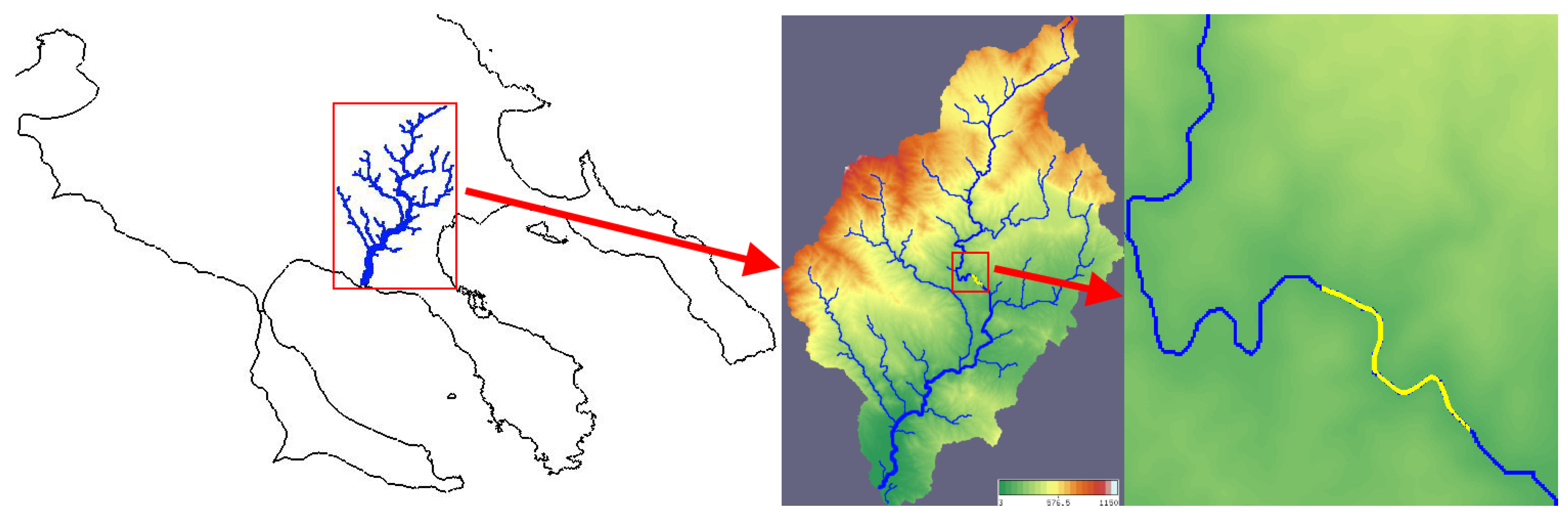
1. Introduction

Flood simulation and river flow one or two-dimensional hydrodynamic modeling require the availability of geometric data describing the morphology of the riverbed as precisely as possible. A significant number of river cross-sections perpendicular to the flow is absolutely necessary though. These cross-sections usually result from field measurements using special measuring equipment, such as theodolites and geographical location devices (GPS—Global Positioning System). Unfortunately, this procedure is costly and time consuming as usually all data gathering field works. Furthermore, the accuracy of the results highly depends on the current weather conditions and the state of the stream/river. For instance, it is very difficult to get reliable measurements from a stream which is full of water and even impossible if the flow is quite fast or even turbulent.

An alternative option is the extraction of the necessary cross-sections directly from Digital Elevation Models (DEM) available. This can be done using appropriate software and has two important advantages over the traditional field study: (a) it can be carried out in a short time period; and (b) the cost is either very low or even zero. The accuracy achieved depends on two factors: (a) the resolution, which dictates the level of detail; and (b) the validity/reliability of the DEM, meaning that it should have been recently formed in order to reflect the present morphology of the area under study. The latter is important because usually DEMs are formed in the past, and, by the time of the study, some, or even many, of the features they include may have changed due to weather conditions or man-made interventions. Another drawback related to the DEMs used for hydrological applications has to do with the way remote sensing, used to assess ground levels, operates above water bodies. When the beam transmitted by the satellite or the airplane is directed towards a water body (e.g., the sea, a river, or a lake), it is reflected on its water surface without being able to go through it and reach the bed’s surface. Therefore, it registers the elevation of the water body’s surface instead of its bed [1,2]. Some of the DEMs have been further processed to overcome this drawback and the water level elevations have been substituted by others, obtained by bathymetry data. This kind of post processing was applied in the DEMs of NASA’s (National Aeronautics and Space Administration) SRTM (Shuttle Radar Topography Mission) [3] project, in which the elevations of the water surface remain for the sea and the lakes but have been replaced for the rivers in a manner that they ensure correct calculation of the flow directions and, consequently, correct delineation of the river network and drainage basins. Despite its drawbacks, this alternative remains particularly attractive since it allows a quick and costless application, especially in the case of a preliminary study. The outcome of this study can lead to a better aimed choice of positions in which field studies will be conducted.

Digital elevation models are essential during the hydraulic modeling of floods as the model’s reliability highly depends on the accuracy level of high-resolution spatially distributed elevation data [4,5,6,7]. Casas et al. [8] studied the effects of the topographic data sources and resolution on 1-D hydraulic modeling of floods. They found out that the contour based digital terrain model (DTM) was the least accurate in the determination of the water level and inundated area of the floodplain. Schumann et al. [9] demonstrated the effects of DEMs on deriving the water level and inundation area. They utilized three DEMs at three different resolutions from three sources (i.e., lidar, contour and SRTM DEM) for a case study area in Luxembourg, where the HEC-RAS (Hydrologic Engineering Center—River Analysis System, US Army Corps of Engineers, USA) 1-D software tool was used to simulate the flood propagation. The results showed that the lidar DEM had the lowest root mean square error (RMSE), followed by the contour DEM and the SRTM. The impact of the different resolutions of DEMs derived by satellite images in the accuracy of the hydraulic modeling of floods has been widely studied. Ali et al. [10], Mercel et al. [11], and Yan et al. [12] investigated various methods to improve the accuracy level of DEMs derived by satellite images, towards developing models of river bathymetry. Andersson et al. [13] applied a new methodology to refine the river cross-section geometry derived by satellite images. In particular, the final product of this work is a MATLAB (programming language, MathWorks, USA) code as an instruction for future use of the slope break method for applications considering river cross-sections. Pramanik et al. [14] presented a methodology for the extraction of cross-sections from DEM for 1-D hydrodynamic studies.

The usual procedure to extract cross-sections from DEMs is mainly done in a manual way and thus is both time consuming and difficult to apply, while its results are not that accurate. In the module RAS-Mapper of HEC RAS [15] for the commercial software ArcGIS (ESRI, Redlands, USA) [16], the user must design by hand the stream’s centerline curve (main stream’s path), the left and right bank’s curve, the left and right floodplain’s curve, and a projection of each cross-section to be created [17]. In the case where a big (long) part of the river is studied, and as the cross-sections need to be as close to each other as possible [18,19], a large amount of cross-sections is required to be sketched by hand. This usually takes lots of time and by no means ensures the cross-sections sketched are perpendicular to the flow or they include the entire case study area. Furthermore, if the results after the hydraulic simulation are not as accurate as expected, forcing the cross-sections to be altered, the whole procedure must be repeated from the beginning all over again.

To simplify this, sometimes exhausting, procedure, several researchers presented alternative techniques for the automatic extraction of cross-sections from DEMs. Gichamo et al. [20] achieved to automatically extract river cross-sections from low resolution DEM of the Advanced Spaceborne Thermal Emission and Reflection Radiometer Global Digital Elevation Model (ASTER GDEM) program (METI—Japan, NASA—US) [21] developing a statistical method to improve the elevation accuracy making use of local elevation information from high resolution DEM. So, that was a hybrid attempt. Pilotti [22] also developed a methodology for the automatic extraction of cross-sections from DEM in order to use them during the hydraulic calculations of the flow after a dam break.

In this paper a new methodology along with the Parametric Cross-sections Extraction Algorithm (PCSEA) developed for the fully automatic extraction of hydraulic cross-sections from DEMs are presented. These cross-sections, in contrast to the previous approaches, are non-planar (also called dog-legged). This fact offers two important advantages: (a) it ensures that these cross-sections are perpendicular to the flow at each subsection; and (b) a much denser sequence of cross-sections can be formed. This second advantage results from the fact that the non-planar cross-sections can come closer to each other compared to their planar counterparts. Furthermore, as the algorithm is basically parametric it can be repeatedly applied simply by altering any of its specified parameters, until the desirable result is achieved. If the algorithm is combined with visual presentation of the results based on an appropriate graphics software, it will provide instant feedback to confirm or modify the design parameters at the time of extraction. This package is considered as a valuable tool for its user (i.e., engineer/decision maker), as it quickly provides preliminary reliable conclusions for any case study area without requiring any former experience or training.

PCSEA together with the Adaptive Cubic Polynomials Algorithm (ACPA) [23] and the Balance Equations with Cubic Polynomials Algorithm (BECPA) are parts of a software pack/tool named “HYDROLOGY”, which has been developed together with the Analytical River Hydraulic Analysis (ARHA) software [24]. HYDROLOGY uses a user-friendly Graphical User Interface (GUI) and allows the creation and hydrological processing of DEMs, delineation of drainage basins, extraction of the river network, extraction of cross-sections, hydraulic calculation, and flood visualization. The cross-sections extracted, together with all related hydraulic parameters can be also exported for further process or simulation using other software tools, such as ARHA or HEC-RAS. Most of the images presented in this paper have been created from screenshots of this software.

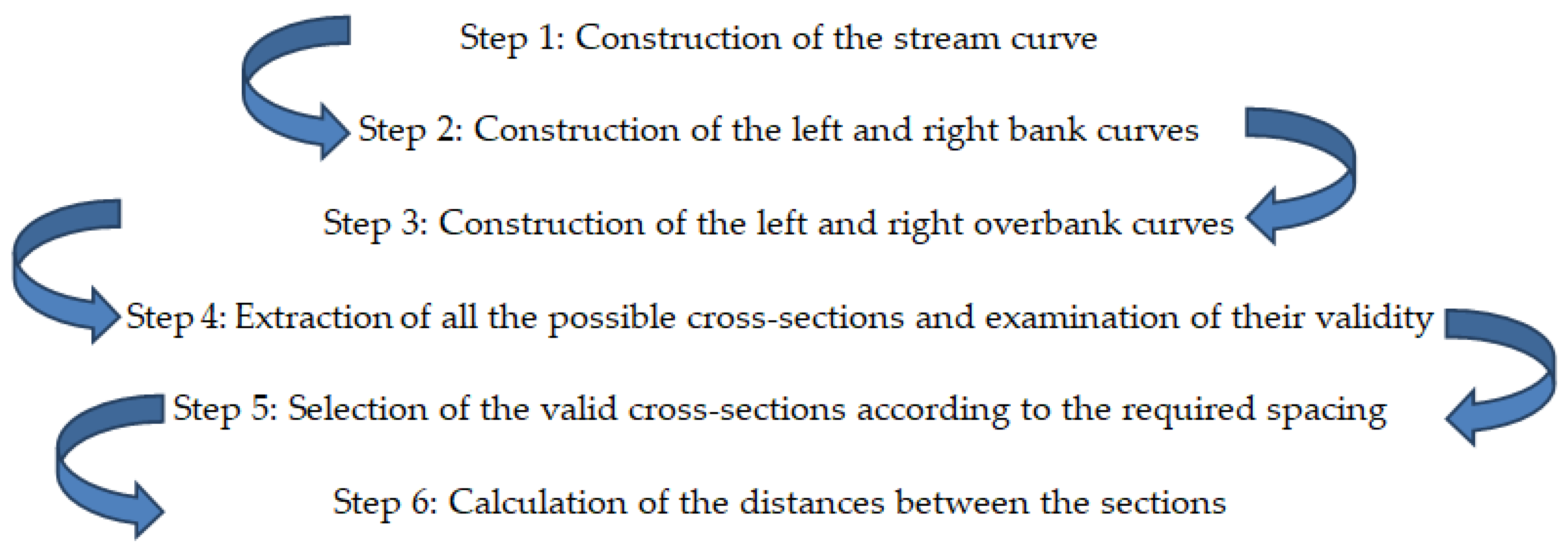
2. The Proposed Approach

The aim of the method proposed here is to make the extraction of river cross-sections from DEMs of a fully automatic procedure. These cross-sections will depend on a set of specified parameters. If the result is not the expected one, then the entire procedure can be repeated as many times as necessary by altering these parameters and crosschecking the result at every loop.

One typical compound or natural cross-section consists of three different subsections (Figure 1): (a) the left overbank (or floodplain); (b) the main channel; and (c) the right overbank.

The general idea is to design/define five curves on the DEM’s plan view: (a) the stream curve; (b–c) the left and right bank curves; (d–e) the left and right overbank curves. These five curves should all have the same number of points and satisfy the following properties:

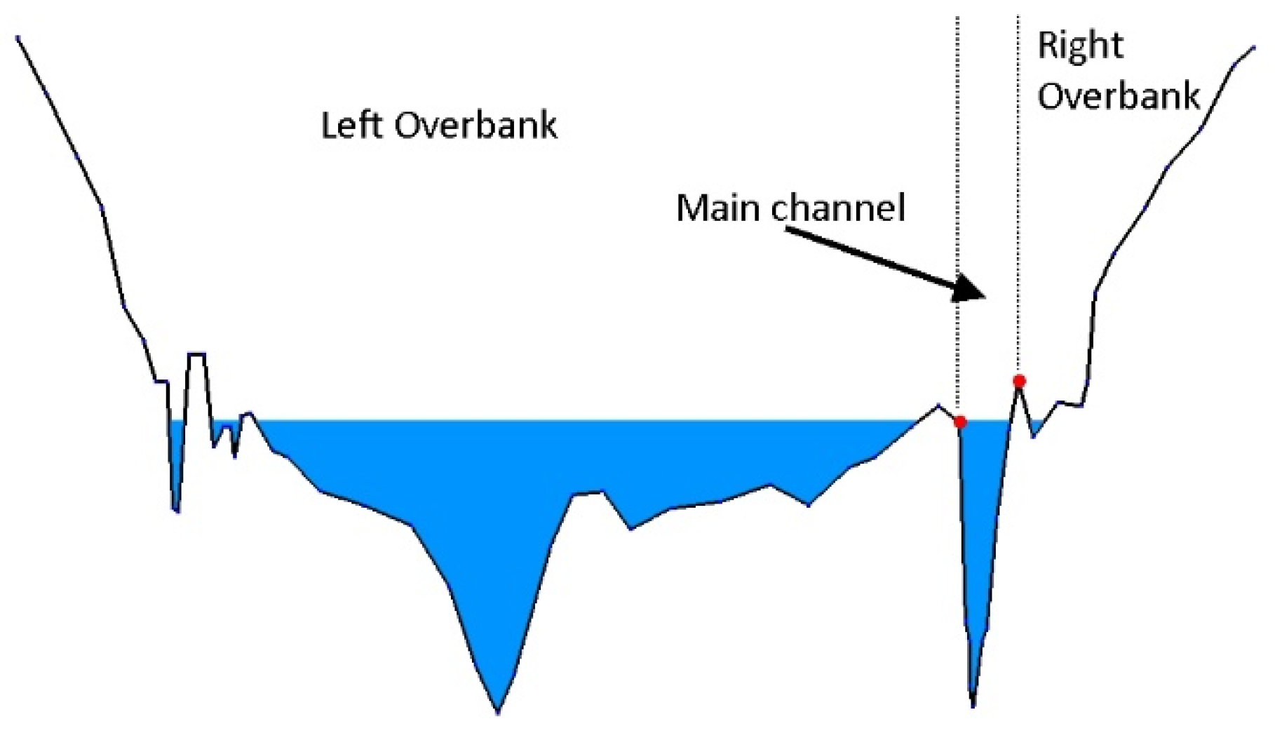
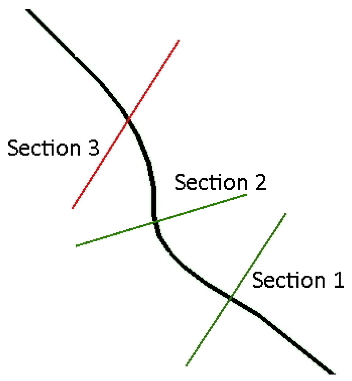
• the main channel of each cross-section should be normal to the stream curve;
• the limits of the main channel (banks) for each section should lie on the left and right bank curves, respectively;
• the projection of each point of either the left or the right bank curve on the stream curve should be the corresponding point (point with the same index) of the stream curve;
• the ending points of each section should be on the left and right overbank curves;
• the projection of each point of the left overbank curve on the left bank curve should be the corresponding point of the left bank curve; and, finally,
• the projection of each point of the right overbank curve on the right bank curve should be the corresponding point of the right bank curve.

These six properties ensure that, if a cross-section is created by connecting the points with the same indexes from the left overbank, left bank, right bank, and right overbank curves, then, this cross-section will be perpendicular to the flow of the main channel (properties 1 and 3), perpendicular to the flow inside the left overbank (property 5), and perpendicular to the flow inside the right overbank (property 6). The whole procedure can be outlined in the six steps shown in Figure 2.

2.1. Construction of the Stream Curve

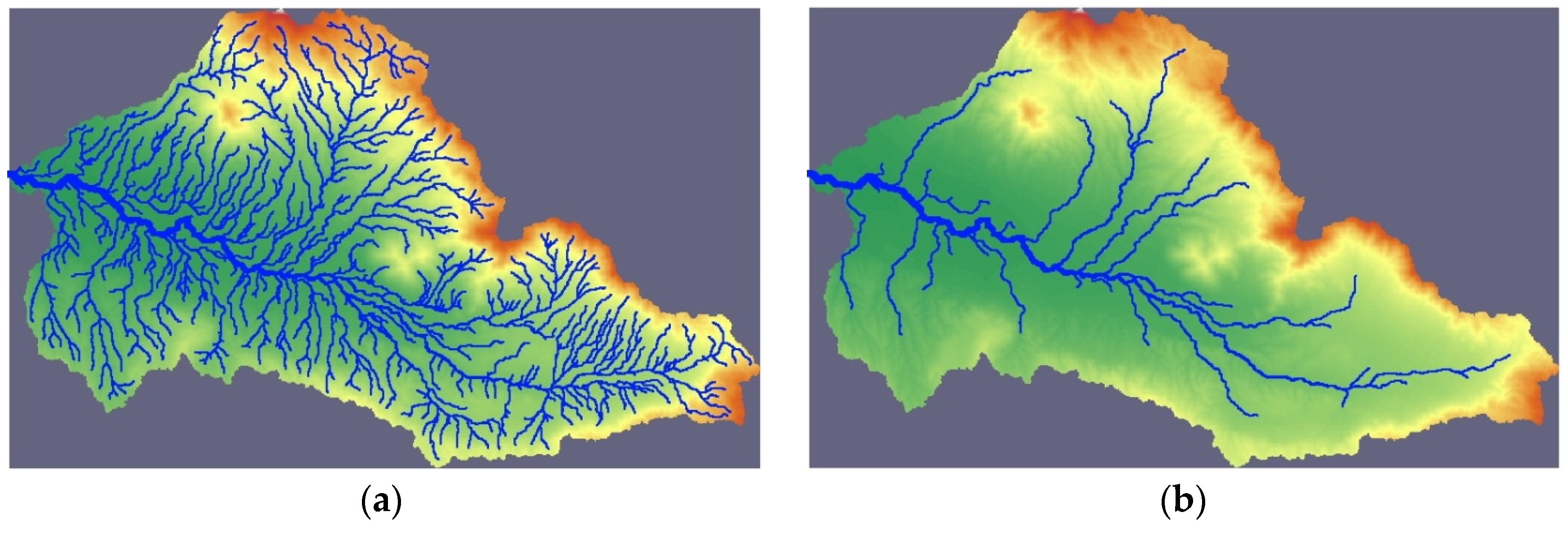
2.1.1. Stream Selection

The first component that needs to be defined is the stream’s path. Although the path can be arbitrarily defined, it is wiser to use hydrological techniques to automatically detect it. This can be easily achieved if the flow direction on every cell of the DEM is reliably defined. Flow directions can be calculated by utilizing one of the many algorithms already developed for this purpose [25,26]. Prerequisite for the application of the flow calculation algorithms is to remove the depressions that a DEM contains. The algorithm adopted herein for the depression’s removal is the one proposed by Planchon and Darboux [27], along with the D8 algorithm for the calculation of the flow directions, developed by O’Callaghan and Mark [28], that was further evolved by Jenson and Domingue [29].

When the flow directions are known, it is easy to determine the water flow path from any cell of the DEM. If a drop of water is put in any of the cells, the flow path can be defined by following the directions. Figure 3 shows a part of a DEM with the calculated directions presented as arrows. The drop is put in the upper right corner and follows the path marked with the red dots until it reaches the edge of the model or its final destination (i.e., sea or lake).

Another algorithm usually applied when hydrological processing is conducted using DEMs is the one that allows extraction of the river network. When the flow directions have been determined, the flow accumulation [29,30] can be calculated. This is essentially the quantity of water that passes through each cell as it flows downstream to its final destination. All the cells of the model will have an accumulation value depending on their position in their drainage basin. The cells that belong to the watershed will have a value of zero, since no other cells drain to them. The cell with the highest value will be the exit cell of the drainage basin since all other cells drain in it. The rest of the cells will have a lower value. Figure 4 shows the same part of a DEM presented in Figure 3. The left table includes the flow direction, while the right one includes the calculated accumulations. The exit point has the greatest accumulation since all the rest 35 cells drain in it. The cell in which the exit point drains has an accumulation value, which is equal to the total number of cells, in this case 36.

The entire river network can be visualized by applying a threshold for the accumulation value. Every cell having an accumulation value greater than the threshold will appear, while the rest will remain hidden. A low threshold value will result in a denser network, since more cells will appear, while a high threshold value will result in a sparser network. Figure 5a shows the DEM of the drainage basin of river Anthemoundas in the city of Thessaloniki, Greece. The accumulation threshold is low; therefore, the network appears dense. In Figure 5b, the same network appears sparse as the threshold value used is twenty times bigger compared to Figure 5a. In both figures, the cell thickness is proportional to the accumulation value; therefore, cells with greater accumulation values appear thicker.

Three different stepwise processes are proposed for the automatic definition of a stream, that all rely on the existence of the flow directions as described above. In addition, the second and third options rely on the existence of the flow accumulations that have been calculated previously. These three options are:

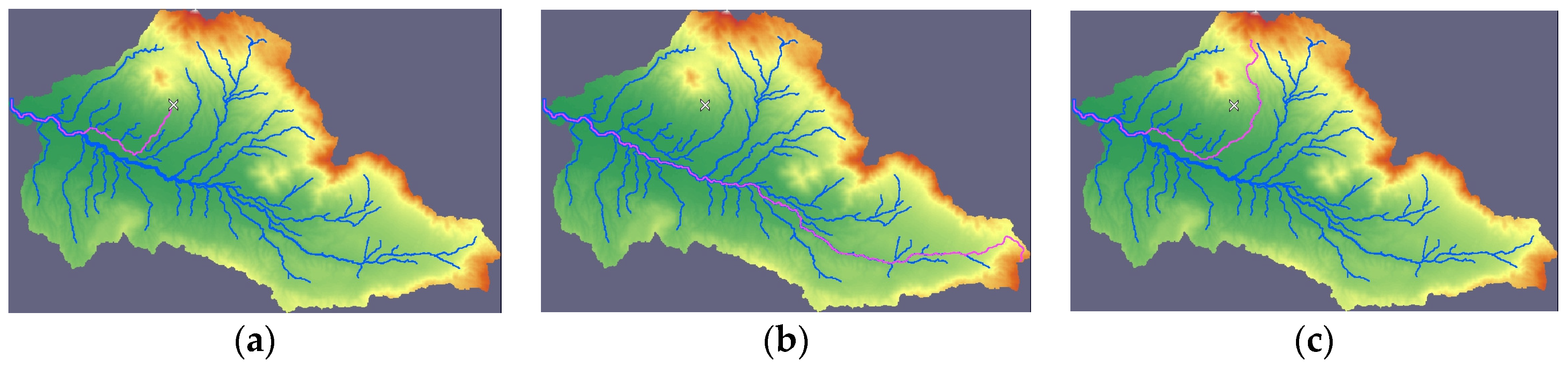
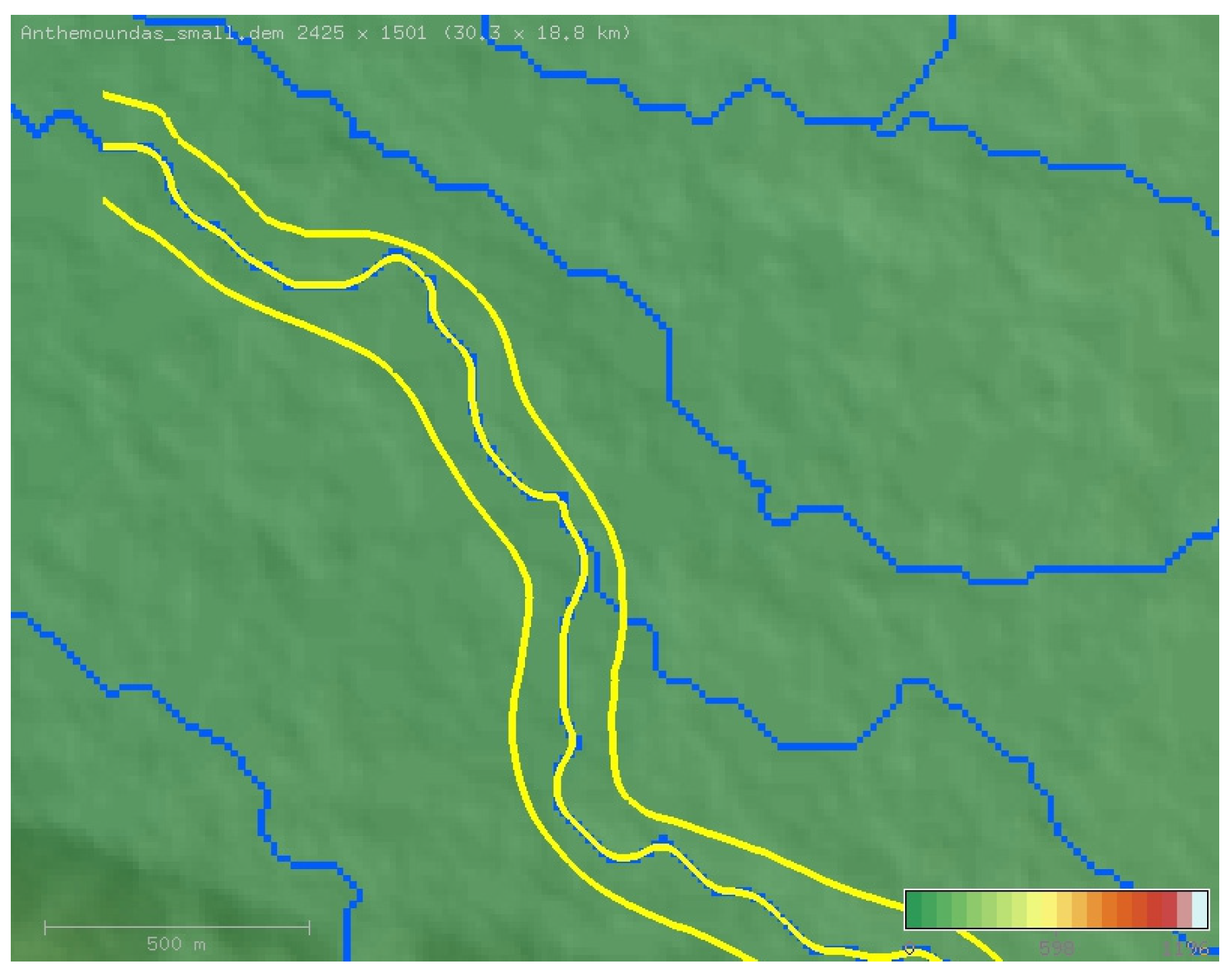
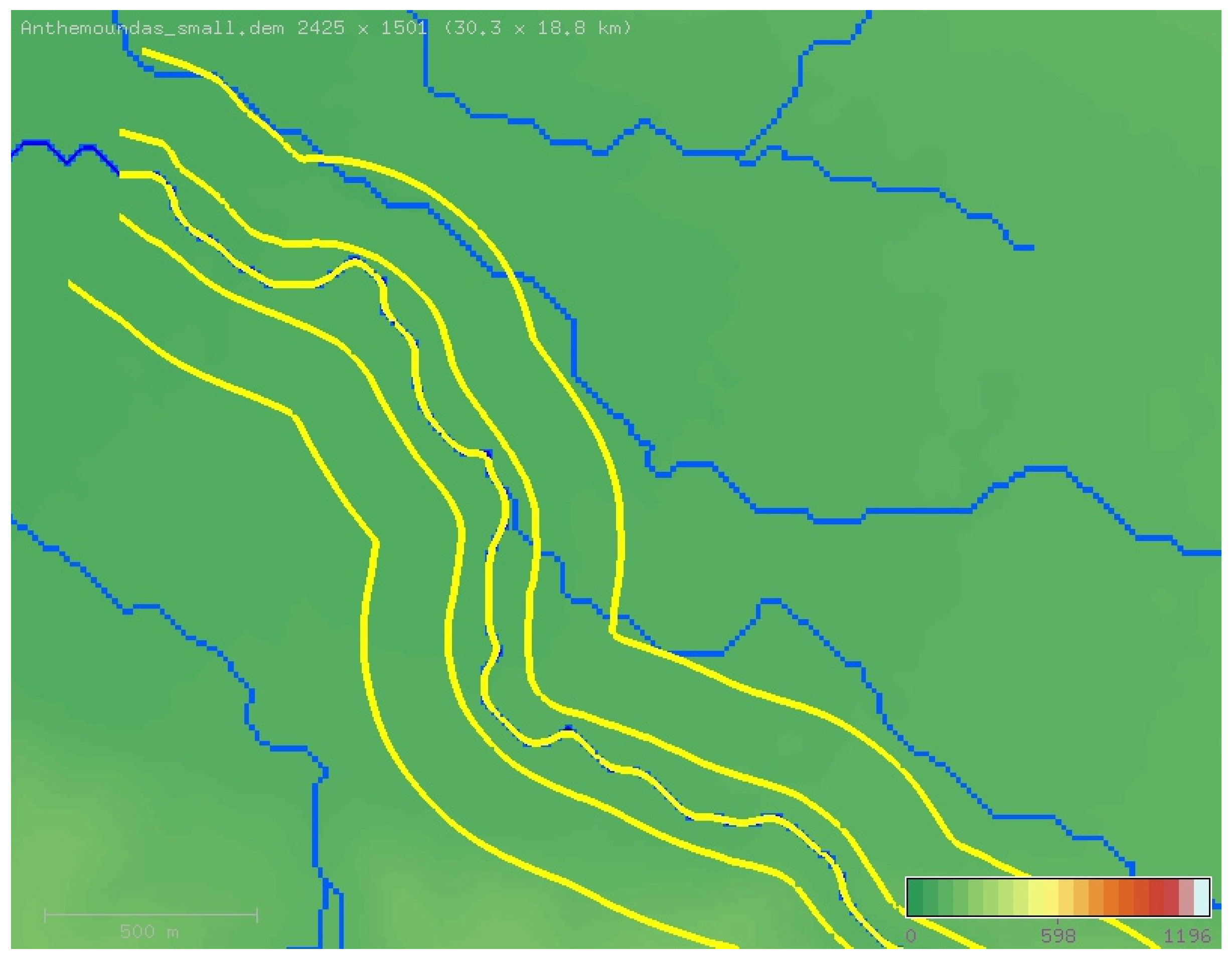
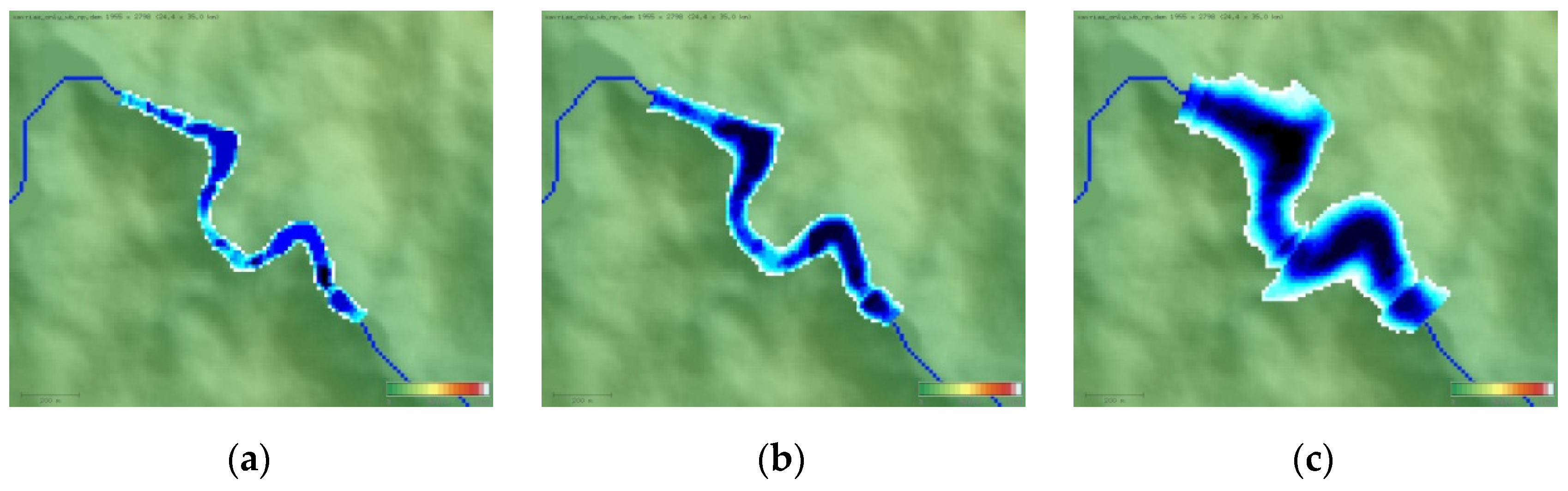
• Route Downstream: This is the simplest process to apply. One cell of the DEM is selected, and then the rest of the path is determined by following the flow directions as described above. Figure 6a shows the stream defined applying this option. The river network appears in blue color, while the selected stream, which appears in purple, extends from the point of selection (white X) until the exit point (pour point) at the western edge of the drainage basin.
• Main Stream: After one cell is selected, the path is determined by following the flow directions as described above until the exit point is reached. Then, the path is reversely followed from downstream towards upstream. At every junction cell, the path followed is the one with the higher accumulation value. Figure 6b shows the stream defined applying this option for the same point of selection (white X) like before. It extends from the watershed till the exit point.
• Nearest Stream: After one cell is selected, the nearest visible stream is searched. The visible streams depend, as explained, on the value of the accumulation threshold value. The path of the stream found is calculated in both directions. When a junction is reached, while calculating the upstream part, the path selected is the one with the highest accumulation value. Figure 6c shows the stream defined applying this option for the same point (white X) as in the previous two options. The stream extends once again from the watershed till the exit point.

The stream defined, applying any of the three alternative ways presented above, consists of a sequence of n₀ successive cells. A cell is fully described by its coordinates (i.e., row and column), so the stream’s path will have the form of an array containing n₀ pairs of coordinates. As the study area may not include the entire stream; therefore, it can be limited by defining a start point p_start (upstream) and an end point p_end (downstream). Thus, the total number of cells becomes n = end − start + 1. Figure 7 shows the study area (in yellow) which, in this case, is part of the main stream of the drainage basin. The total length is 40 km, while the study area’s length is 10 km. Many methods for the visualization of DEMs exist [31]. To visualize the elevations, the display method selected is the relief map.

2.1.2. Stream Smoothing

As mentioned before, every stream consists of a sequence of successive cells. A cell is considered a successive one if it belongs to one of its neighboring cells. The proposed process restricts the direction to eight distinct alternatives (i.e., N, NE, E, SE, S, SW, W, NW), each one being a multiple of 45 degrees. This fact causes abrupt changes of direction, and, as the cross-sections must be normal to the path, it limits their orientation to these eight particular angles. The method adopted to address this issue is to smooth the stream path by applying an averaging filter. Before applying the filter, the cells must be converted to points, namely the coordinates of the stream path, expressed in rows and columns, reflecting the real-world coordinates (meters or feet) of the cells’ centers. The conversion takes place for all cells according to the following equations:

$$X_i=X_{min}+h_{res}·\left(co{l}_i+0.5\right),$$

(1)

$$Y_i=Y_{min}+v_{res}·\left(ro{w}_i+0.5\right),$$

(2)

where X_min and Y_min are the real-world coordinates of the lower left corner of the DEM; and h_res and v_res represent the horizontal and vertical resolution of the DEM, respectively.

After this conversion is concluded, the stream path will have the form of an array containing n pairs of real-world coordinates X, Y, one pair for each point. The averaging filter requires a single parameter, the radius, and is applied according to the following algorithm: “for each point apart from the first and the last, calculate the average of its coordinates X’ and Y’ from the r previous, the same point and the r next (2r + 1 total points)”, according to the equations:

$$X^{\prime }{}_i=\frac{1}{2r+1}{{\displaystyle \sum }}_{j=i-r}^{i+r}{X}_j,$$

(3)

$$Y^{\prime }{}_i=\frac{1}{2r+1}{{\displaystyle \sum }}_{j=i-r}^{i+r}{Y}_j.$$

(4)

The coordinates calculated following this procedure substitute the original coordinates of the points and any abrupt changes of direction become blunted resulting in a smoother path. This feature can be deactivated by setting the smoothing radius to zero. As the radius rises, the path becomes smoother, but at the same time the points move further apart compared to their original positions. Figure 8 shows a part of a stream for which smoothing filters with different radius values have been used. The original cells of the stream appear in blue, while the smoothened curve appears in green. In Figure 8a, the smoothing radius is set to zero, so no smoothing takes place. It obvious that the changes in direction are always multiples of 45 degrees. In Figure 8b–d, the smoothing radius is set to one (1), two (2), and five (5), respectively. It is apparent that, as the radius rises, the curve moves further away from the original stream points.

2.2. Construction of the Left and Right Overbank Curves

Each bank curve should satisfy property 3 (as stated in Section 2.1.1), namely the projection of each point on the stream curve should be the corresponding point (i.e., point with the same index) of the stream curve. This ensures that the cross-section’s main channel plane will be perpendicular to the flow and can be achieved if each point of this curve lies on a line that is normal to the stream curve and passes from the corresponding point. Therefore, its points must be determined by offsetting the points of the stream curve by a certain distance along these normal lines. This distance cannot be the same for each cross-section, as the width of the channel varies from cross-section to cross-section, being narrower or wider depending on the morphology of the stream. The method developed herein is an attempt to automatically detect the stream’s bank according to the profile of each cross-section and then connect the points to design the bank curve. Then, the curve is validated and smoothed.

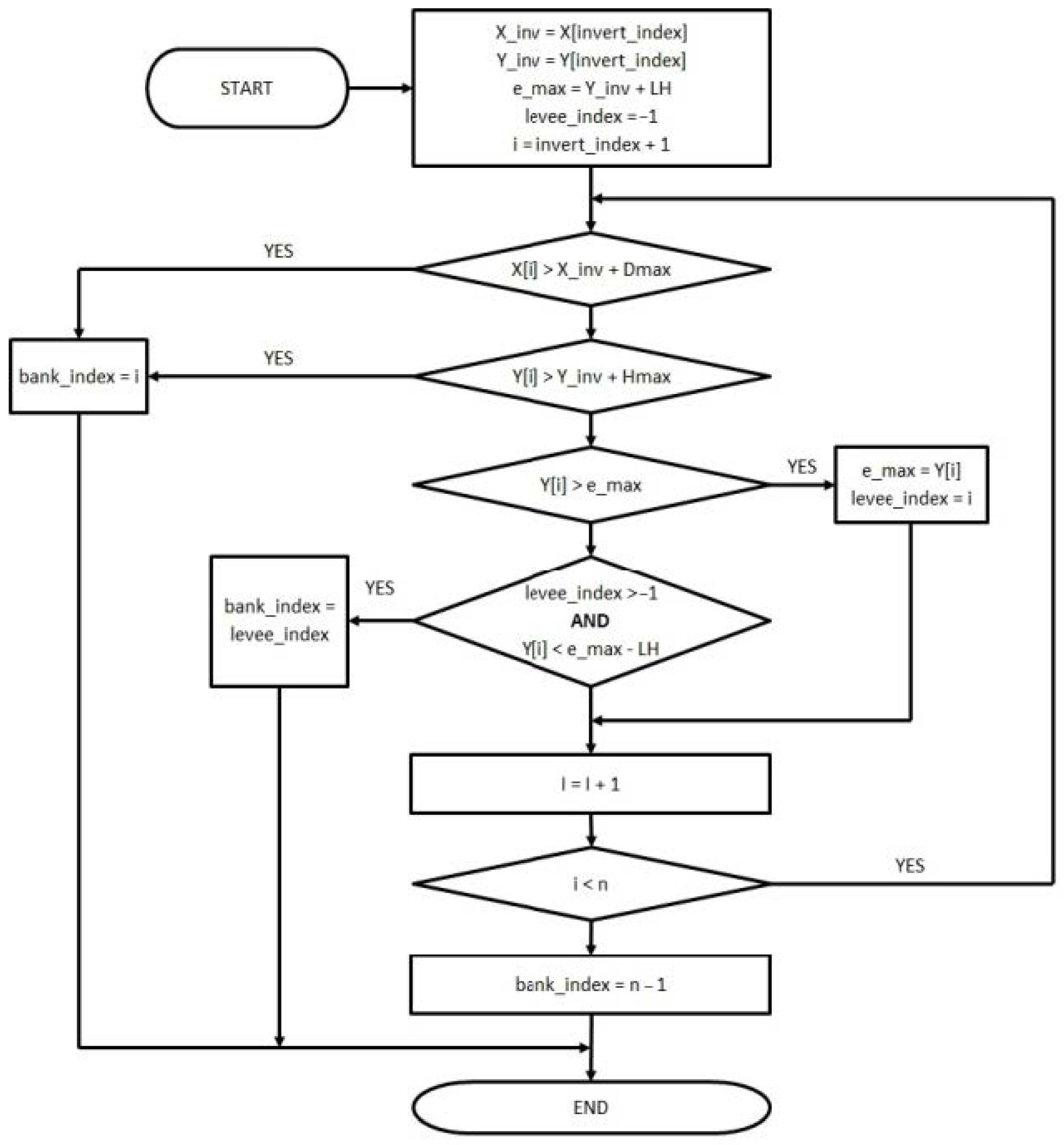
2.2.1. Automatic Detection of Left and Right Bank

First, the stream direction at each point is calculated. The stream curve consists of a series of n successive points. In each one of these points, the angle φ between the stream and the horizontal line can be calculated using the following equation:

$$\phi =\arctan \left(\frac{y_{i+1}-y_{i-1}}{x_{i+1}-x_{i-1}}\right),$$

(5)

where x_i−1, y_i−1, and x_i+1, y_i+1 are the coordinates of the previous and the next point, respectively. With this angle calculated, it is easy to compute the unit vector that is passing from this particular point and is normal to the stream with direction to the left (looking from upstream to downstream):

$$\stackrel{\rightharpoonup }{v_{Left}}=\langle \cos \left(\phi +{90}^o\right), \sin \left(\phi +{90}^o\right)\rangle .$$

(6)

Similarly, the unit normal vector with direction to the right is calculated:

$$\stackrel{\rightharpoonup }{v_{Right}}=\langle \cos \left(\phi -{90}^o\right), \sin \left(\phi -{90}^o\right)\rangle .$$

(7)

Figure 9 shows a part of the stream curve. The angle φ at point p_i is calculated from the coordinates of points p_i−1 and p_i+1. The normal vectors $\stackrel{\rightharpoonup }{v_{Left}}$ and $\stackrel{\rightharpoonup }{v_{Right}}$ are also shown.

The following procedure takes place in both directions left and right. Beginning from the current point of the stream p_i and moving along the normal vector $\stackrel{\rightharpoonup }{v}$ by a small distance ds, a series of successive points q_j are created according to the following equation:

$$q_j=p_i+\stackrel{\rightharpoonup }{v}·ds, j = 1, 2, \dots .$$

(8)

The distance ds is selected smaller than the distance between the cells (resolution) so that the transitions between the point elevations are smooth. For each of these points the elevation can be calculated using various methods (i.e., Nearest Neighbor; Bilinear Interpolation; Bicubic Interpolation, etc.). The simplest one is the Nearest Neighbor since it only requires finding the cell that is closer to the specified point and using its elevation. This way though, all successive points that fall into the same cell will have the same elevations. Furthermore, considering the fact that the DEM cells usually have integer elevations, successive points will either have the same elevation or will have abrupt changes between them. Figure 10 shows a series of nine successive points. With the Nearest Neighbor method, points 1, 2, and 3 will have elevation Y1, points 4, 5 and 6 will have elevation Y2, point 7 will have elevation Y3, and, finally, points 8 and 9 will have elevation Y4. It is obvious that each point has the elevation of the cell in which it is contained.

Bicubic Interpolation allows calculation of the elevations with very smooth transitions but has the drawback that it can result in elevations that are higher or lower than those of the neighboring cells. Figure 11 shows the elevations of points 1, 2, and 3, which have been calculated from the elevations of points A, B, C, and D applying the Bicubic Interpolation method. Point 1 has a lower elevation and point 3 has a higher elevation than its two neighbors, respectively.

As the Bilinear Interpolation method results in smooth transitions without calculating elevations outside the limits of the neighboring cells, it has been chosen for the calculation of the elevations in the present paper. First, the four neighboring cells, the centers of which surround the specified point, are located. In Figure 12, the point where elevation is to be calculated with known coordinates x and y is pinpointed as a red dot. The centers of the surrounding cells with known coordinates and elevation appear as black dots. First, the point’s unit square coordinates η and ξ are calculated as:

$$\eta =\frac{x-x_1}{x_2-x_1},$$

(9)

$$\xi =\frac{y-y_1}{y_2-y_1}.$$

(10)

These coordinates span in the range [0,1]. Next, elevation Ε is calculated as:

$${\rm E}={{\rm E}}_{11}\left(1-\eta \right)\left(1-\xi \right)+{{\rm E}}_{21}·\eta \left(1-\xi \right)+{{\rm E}}_{12}\left(1-\eta \right)\xi +{{\rm E}}_{22}·\eta ·\xi .$$

(11)

After the elevation of each point is calculated for either direction, the automatic definition of the banks takes place. In compound hydraulic cross-sections, the banks are essentially the borders between the main channel, where the flow normally takes place and the floodplains where flow exists only in cases of high discharges when the water volume transferred exceeds the carrying capacity of the main channel. Due to of the corrosive nature of water and sediment, the friction coefficient in the main channel is lower than the one of the floodplains. Therefore, without this being restrictive, the separation of the main channel from the floodplains in compound cross-sections takes place basically to allow the definition of different friction coefficients for each part. Thus, parallel flows with different velocities occur, as expected. When the channel bed is inside a deep canyon, most of the time the water level is more or less constant, and the water corrodes only the bed’s deeper part. In this case, the bank is considered the point where this water level intersects the sidewall. An additional feature of the bank may be the existence of a levee. As time passes, water corrodes the submerged part, causing the channel bed to move deeper, while sediment stacks on the bank and creates a levee, after which the elevation drops.

Having defined the appropriate parameters for these two features, the bank can be automatically detected. In particular, the maximum height of the bank from the deeper part of the channel bed (Max Height) and the minimum height of the levee (Levee Height) can be defined. Figure 13 shows the series of points of the cross-section, where the deepest point (invert) is the blue dot, while the banks are the red dots. On the right, a levee is detected; therefore, the bank is set on its ridge. On the left, no levee can be detected; therefore, the bank is set at the point where the height from the invert equals the defined value.

In the case that no bank can be detected through the procedure above, the bank is set at the point where the horizontal distance from the invert exceeds a predefined value (Max Dist). This appears in Figure 14, where the right bank cannot be detected with either of the two aforementioned conditions; therefore, it is set at the point where the distance from the invert exceeds the value defined.

To summarize, the three following parameters are defined: (a) the minimum levee height (Levee Hgt.) H_L; (b) the maximum height from the channel bed (Max Height) H_max; and (c) the maximum horizontal distance (Max Distance) D_max. Then, all points in both directions are examined until one of the following conditions is satisfied:

• A. Levee detection: Moving away from the invert, if two points p₁ and p₂ with elevations h₁ and h₂ are found for which h₂ < h₁ − H_L, then p₁ is considered to be the bank.
• B. Maximum height from invert: Moving away from the invert, if one point p with elevation h is found for which h > h_invert + H_max, then p is considered to be the bank.
• C. Maximum horizontal distance from invert: Moving away from the invert, if one point p with distance from the invert is d > D_max, then p is considered to be the bank.

Figure 15 presents the logic diagram of the right bank detection algorithm. Arrays X and Y with n positions each, ranging from 0 to n − 1, contain the horizontal distances and the elevations of the cross section points, respectively. The invert index is the index of the lowest point of the river’s bed. At the end of the algorithm, variable bank_index is set to the index of the point that matches the criteria specified. The algorithm for the left bank is similar but in the opposite direction.

After detecting the left and right bank for each point, all these points are connected to form the left bank curve and the right bank curve, respectively. When the curve laying at the inner side of the stream is defined, it is possible to form closed loops. Thus, the curve will be self-intersecting. In this case, all the points forming this loop are removed and replaced by the intersection point where the loop starts. Hence, all these points coincide, and the curvature is not smooth, but, at the same time, the curve remains valid. Furthermore, the cross-sections that are defined via this procedure are no more planar and extend to two or three planes. Thus, these cross-sections are called dog-legged. This case appears in Figure 16, where points 1, 2, and 3 are offset parallel to the stream path by a distance that is greater than the local curvature radius. When the outer bank curve (left) is formed, these points are projected to A, B, and C, respectively, and the curve is valid. On the other hand, when the inner bank curve (right) is defined, these points are projected to D, E, and F, which belong to the closed loop formed; therefore, they are all replaced by the same point G, which is the intersection point of the curve, the loop is removed, and the curve remains valid. Figure 17 shows the result where the right bank apparently has no smooth curvature, and each of the cross-sections A1G and C3G extend to two planes.

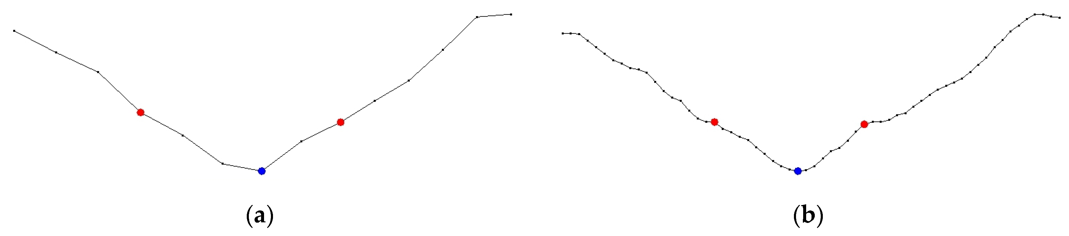
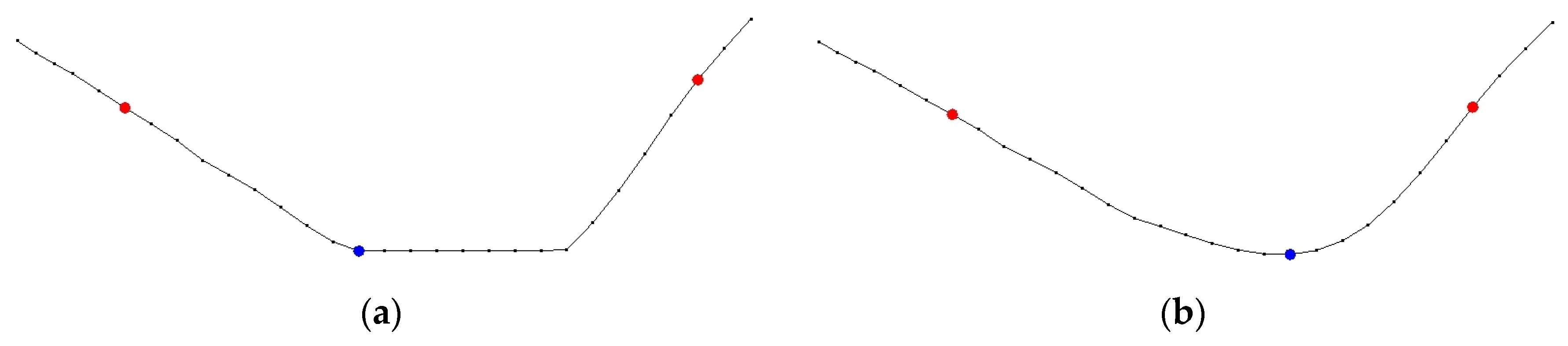
2.2.2. Banks’ Curve Smoothing

The bank curves are formed following this automatic procedure, as explained, can possibly contain points with abrupt changes of curvature. As with the stream curve, smoothing of these curves can be done by applying an averaging filter. Likewise, if the radius is set to zero, no smoothing occurs, while, on the contrary, if a big radius is selected, then, although the visual result is better, the curve moves further away from the original points.

After applying the averaging filter, the curve is examined for possible local abrupt changes of curvature. If such changes are detected, an additional local averaging filter is used to blunt them. In particular, all successive triplets of curve points are examined, and, in case the angle formed by these points is acute, the local averaging filter is applied to the middle point so that the angle is blunted. This procedure takes place as many times as necessary until no acute angles exist. The minimum allowed angle is defined by an appropriate parameter (Min Angle), while, for the application of the local smoothing filter, the smoothing radius is always set to one. Figure 18a shows a part of the curve before a smoothing takes place. The angle 2–3–4 formed is smaller than the predefined minimum angle; hence, the local averaging filter is applied on point 3. The result appears in Figure 18b, where the coordinates of point 3 have changed, and the new point is 3′. Angle 2–3′–4 is greater than before, and the curve becomes smoother.

After the automatic detection and the smoothing, the two bank curves have been created. Figure 19 shows the final shape of the banks for one part of the stream on the DEM’s plan view after the implementation of the procedures presented above. The stream curve and the two bank curves are displayed in yellow. The distance between the curves does not remain constant as it depends on the morphology and the parameters defined.

2.3. Construction of the Left and Right Overbank Curves

The overbank curves should satisfy properties 5 and 6 (as stated in Section 2.1.1), namely the projection of each point on the left or right bank curve should be the corresponding point (i.e., point with the same index) of the left or right bank curve. This ensures that the cross-section’s left or right overbank plane will be perpendicular to the respective flow. This can be achieved if each point of this curve lies on a line that is perpendicular to the left or right bank curve and passes from the corresponding point. Therefore, their points must be determined by offsetting the points of the respective bank curve by a certain distance along these normal lines. This distance simply defines the length of each overbank area and therefore can be the same for all the cross-sections. Two parameters are needed for this purpose one for the left and one for the right distance. Each overbank curve is calculated by offsetting the respective bank curve. As explained before, when this offset takes place at the inner side of the curve and the offset distance is greater than the local curvature radius, self-intersecting closed loops occur. In this occasion, the loops are removed, and all their points are replaced with the intersection point at the beginning of the loop. It should be noted that a long distance reduces the possibility of flood, assuming that the elevations rise by moving further away from the bank.

2.4. Extraction of Cross-Sections

At this point all five curves have been defined: the stream (C curve), the two banks (E and F curves for left and right), and the two overbanks (D and G curves for left and right). As mentioned before, all of them include the same number of points. If the points from all curves with the same index are connected from left to right (i.e., left overbank; left bank; right bank; and right overbank), three successive straight-line segments are formed, which are not necessarily collinear. These are the projections of the left overbank area, the main channel, and the right overbank area of a compound or natural cross-section. From the way these curves are formed, it can be concluded that these segments are perpendicular to the curves and, consequently, perpendicular to the flow that takes place in each of these three areas.

Figure 20 shows an example of the stream curve (colored in blue), bank and overbank curves (colored in black), and the sections formed (colored in red). The bank points A and B are sought along the line that is perpendicular to the thalweg (shown in Figure 9). The direction of the flow FG is assumed to be coincident with the direction of the thalweg; hence, the banks detected lie on the line that is perpendicular to the flow. Since FG and AB are perpendicular, the cross section’s main channel is also perpendicular to the flow. Each bank curve is defined by the bank points detected. The bank curve is offset parallel by a specified distance to create the overbank curve; thus, the lines connecting points with the same index are bisectors of the angles formed by adjacent points of each curve. In this example, BD is the bisector of angle CDE. The flow in the overbank area is assumed to be perpendicular to the bisector, so, in this example, HI is perpendicular to BD; hence, the overbank is perpendicular to the respective flow.

Figure 21 shows all five curves in yellow in their final form for a part of the stream on the DEM’s plan view.

A cross-section can be formed for each point of the stream curve following six steps: (1) examination of the angle between the cross-section and the stream; (2) calculation of the coordinates of the cross-section; (3) examination of the maximum water depth of the cross-section; (4) channel bed restoration; (5) addition of levees; and (6) removal of ineffective areas. The cross-section for the ith point of the stream curve is constructed with the following procedure: The limits of the section are on the curves D, E, F, and G, and, in particular, they are the points d_i, e_i, f_i, and g_i with coordinates (xd, yd), (xe, ye), (xf, yf), and (xg, yg), respectively, as shown in Figure 22. The cross-section projection consists of the three successive lines d_i–e_i, e_i–f_i, and f_i–g_i.

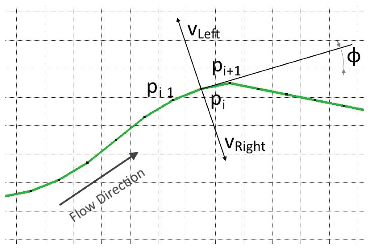
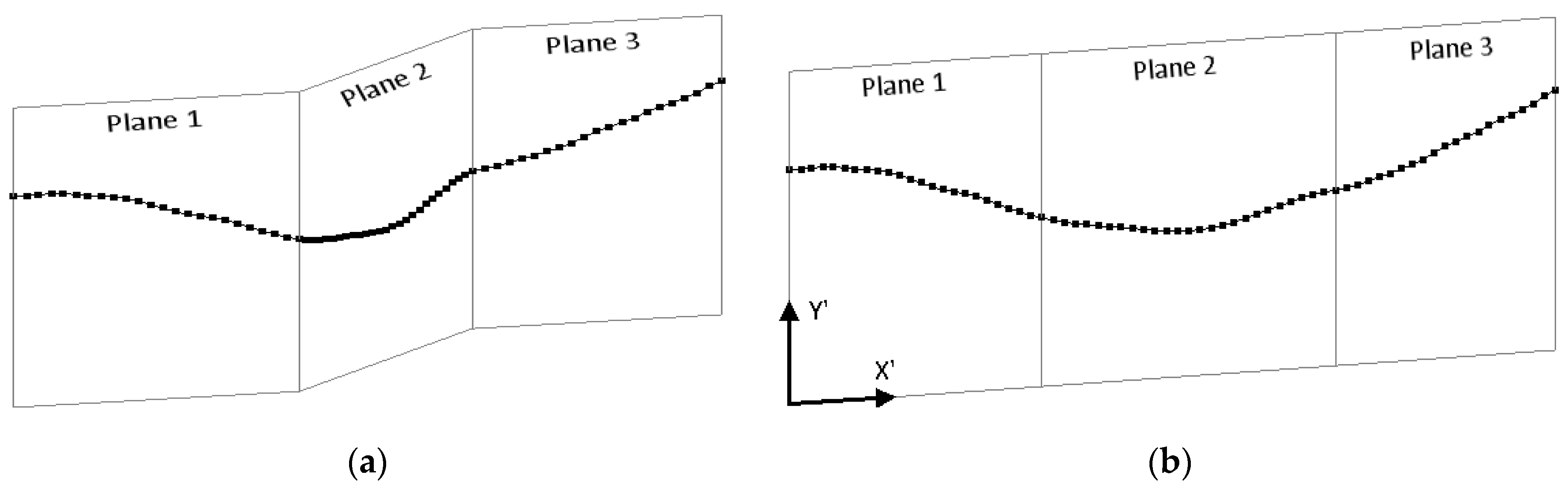
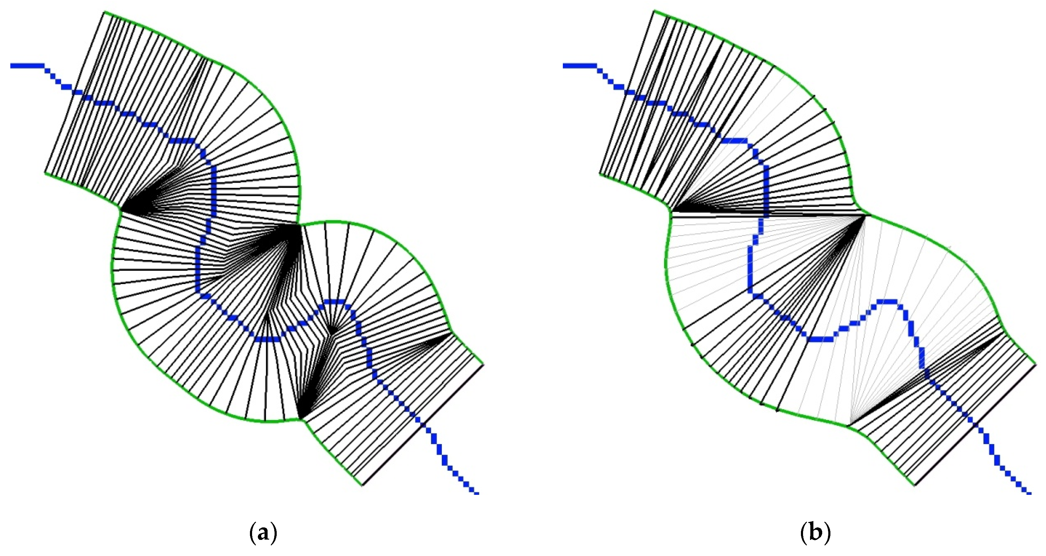
2.4.1. Examination of the Angle between the Cross-Section and the Stream

As explained before, curves D, E, F, and G are formed to ensure that the cross-section is perpendicular to the stream. However, due to the smoothing and removal of self-intersecting loops, this is not always the case. At this point, the angle between e_i–f_i and the stream needs to be examined and compared to the least acceptable value defined (Min Angle). Ideally, this angle should be 90°. If it is less than Min Angle, the cross-section does not comply with the restriction set and should be rejected. Figure 23 shows a part of the stream and three cross-sections. Cross-sections No 1 and 2 (green) are almost perpendicular to the path, while No 3 (red) is not, so it is rejected.

2.4.2. Calculation of the Coordinates of the Cross-Section

Each of the three straight lines of the projection d_i–e_i, e_i–f_i, and f_i–g_i (referred hereafter as S1, S2, and S3) is divided into smaller segments of equal length so that their length is shorter or equal to the specified parameter (Segment Length), and, for each point, the elevation is calculated with bilinear interpolation. The applied procedure is the same as the one described in Section 2.2.1. Each point of the section has known coordinates x, y in the plan view, and its surrounding cells have elevations E11, E12, E21, and E22, as shown in Figure 12. Its elevation E is calculated with Equation (11) after calculating the unit coordinates η and ξ with Equations (9) and (10), respectively. The value of the Segment Length parameter affects the level of detail for the calculated cross-section. The smaller this length the smoother the transition from each point to the next appears. In Figure 24a,b, the same cross-section has been created with a long and a short length, respectively. It is apparent that, in the second case, the transitions are smoother, and the level of detail is higher.

After calculating the elevations, all the coordinates of the cross-section can be calculated, too. Each one of the S1, S2, and S3 defines a different plane, which is normal to the plan view and passes from the corresponding line. This renders the cross-section three-dimensional (Figure 25a).

The cross-sections used in hydraulic calculations are considered two-dimensional. This means that they are defined on a single unfolded plane; therefore, the three planes need to be aligned, namely to become coplanar and successive (Figure 25b). To achieve this, the coordinate system (CS) must change from the three-dimensional (X-Y-Z) of the DEM (Figure 22), to the two-dimensional (X’-Y’) of the cross-section, which is shown in (Figure 25b). The coordinate X’ of each point is in fact the horizontal distance of the point from the beginning of the section and is calculated along the projection lines S1, S2, and S3. For the points that lie on the first plane (Plane 1—left floodplain) this is the distance of each from point (xd, yd). For the points that lie on the second plane (Plane 2—main channel), this is the distance of each from point (xe, ye) plus the length of S1. Finally, for the points that lie on the third plane (Plane 3—right floodplain), this is the distance of each from point (xf, yf) plus the length of S1 plus the length of S2. Alternatively, coordinate X’ can be calculated with the following equation:

$$X^{\prime }{}_i={{\displaystyle \sum }}_{j=2}^i\sqrt{{\left(x_j-x_{j-1}\right)}^2+{\left(y_j-y_{j-1}\right)}^2},$$

(12)

where x_j, and y_j are the original coordinates of the points on the three-dimensional CS (Χ-Υ-Ζ) of the DEM. The Y’ coordinate is the same as the Z coordinate of the DEM, namely the elevation, and was calculated with bilinear interpolation, as described previously.

After the coordinates of the cross-section have been calculated, the invert and the banks are re-defined by examining the three conditions (i.e., minimum levee height, maximum depth from invert, and maximum horizontal distance from invert). The banks defined following this procedure do not necessarily coincide with points e_i and f_i.

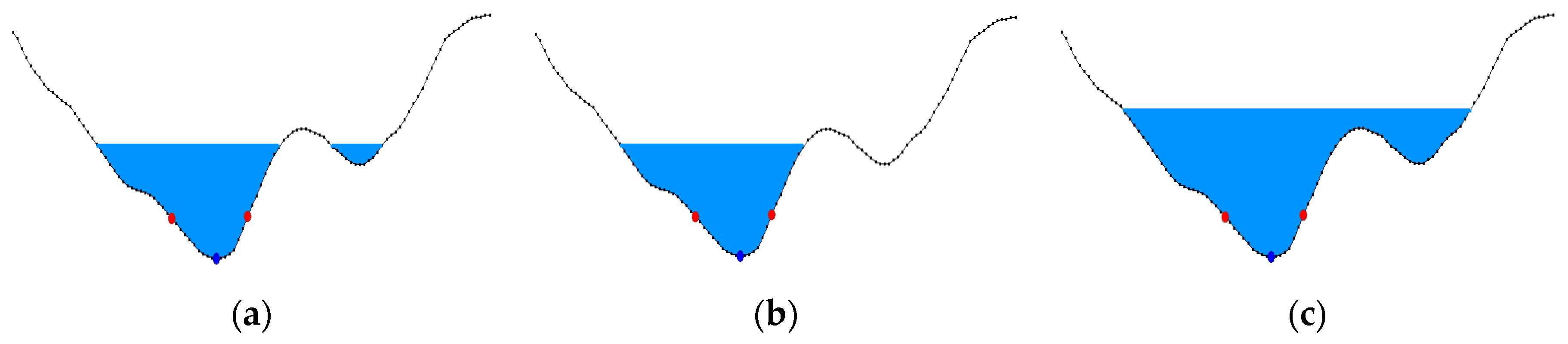
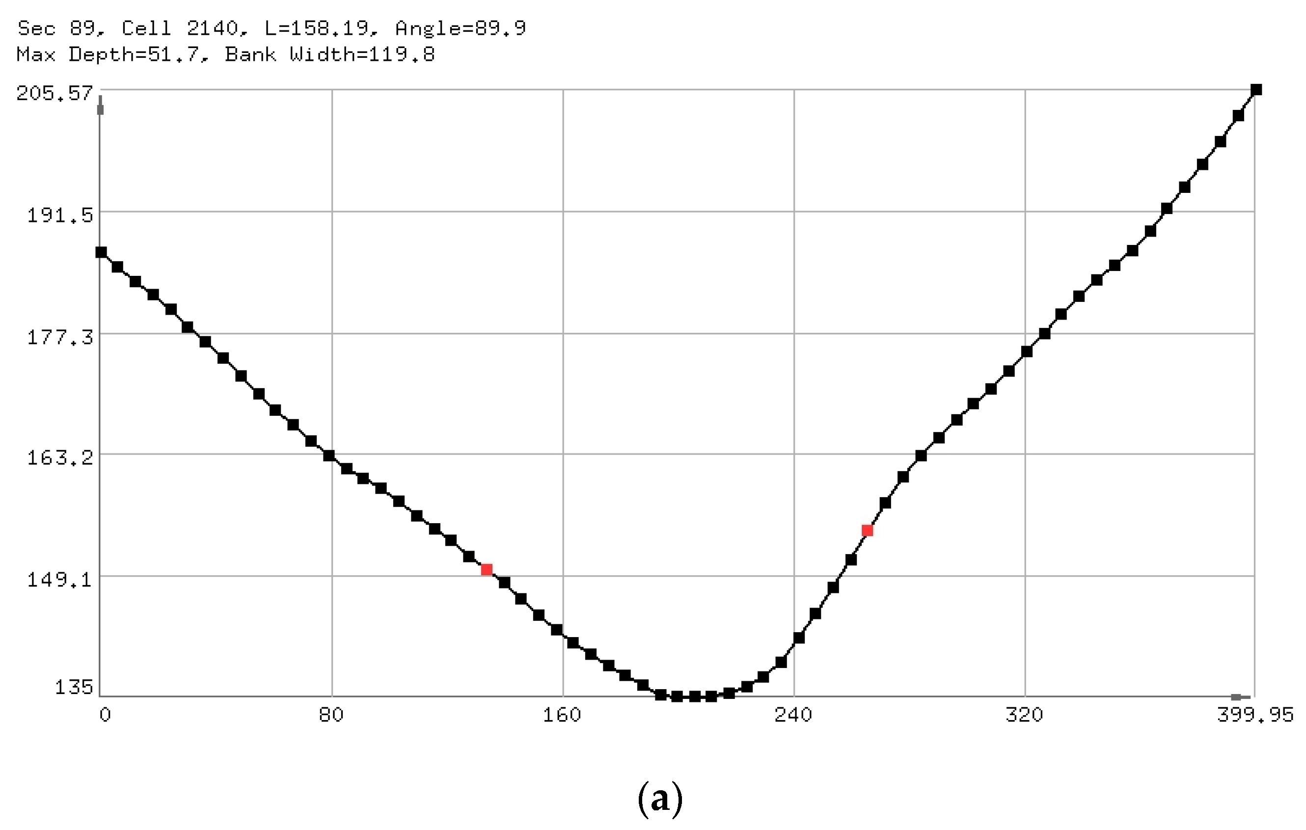
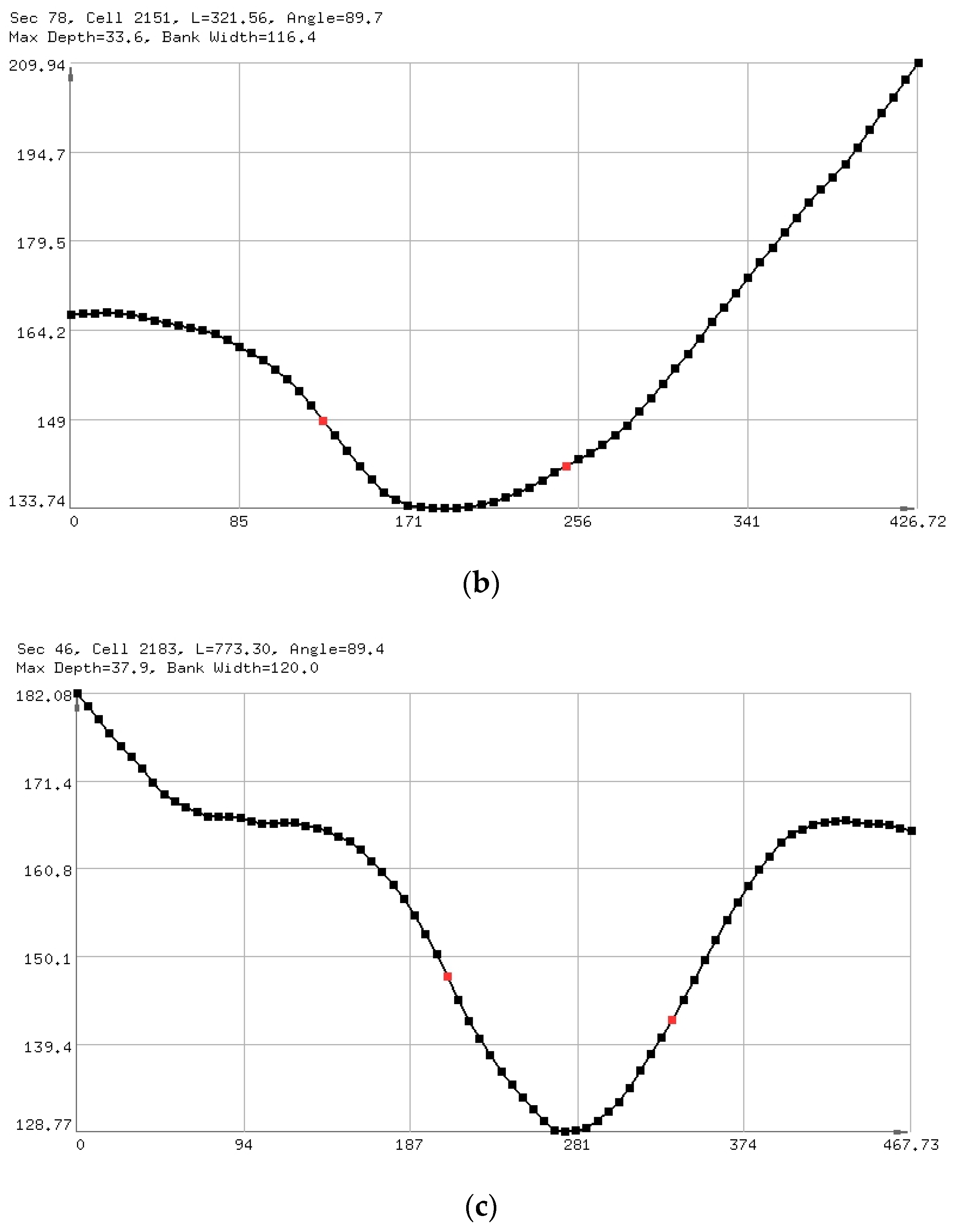
2.4.3. Examination of the Maximum Water Depth of the Cross-Section

The streams and rivers extracted from DEMs are sometimes passing over flat areas where there is no open channel, or the existing channel is very shallow. If a cross-section is defined on a flat area, then it will not have the carrying capacity necessary to convey the water, and it will always flood. Cross-sections of this kind can be rejected by examining their maximum water depth and comparing it to the least acceptable value defined (Least Depth). First, the deepest point of the channel is determined (invert), and then the elevation differences H₁ and H₂ between the highest point left and right, respectively, from the invert are calculated. The maximum depth is the least of H₁ and H₂. This depth is compared to the parameter Least Depth, and, if it is less than this value, then the cross-section is rejected. This restriction can be deactivated by setting this parameter to zero. Figure 26 shows the heights H₁ and H₂. H₁ is less than H₂; therefore, this is the maximum possible water depth.

2.4.4. Channel Bed Restoration

During the automatic determination of the cross-sections, sometimes the channel bed appears unnaturally flat. This can happen for two reasons. The first one is that the elevations of a DEM are usually rounded to the nearest integer and, consequently, a difference of less than one meter (or foot) cannot be shown and appear to be zero. The second reason is that, during the remote sensing of the ground elevation from the satellite or the airplane, the beam transmitted cannot penetrate the water surface, and it is reflected, registering the elevation of the water surface instead of the channel’s bed. In both cases, the real conveyance of the section is greater than the one assessed, and, in order to correctly define it, the depth of the section must be increased. For this reason, a method that allows the channel’s bed shape to be properly modified so that it becomes parabolic has been developed. Four boundary conditions are used, two at the edges of the flat area and the two points next to them (outside the flat area). Figure 27 shows the points used for the boundary conditions, where the edges are shown with red dots and the points next to them with green dots.

From these boundary conditions, the coefficients of a cubic polynomial can be calculated. This polynomial passes exactly from these four points, while it approximates the intermediate ones with a parabolic curve that lies at lower elevations. This allows substitution of the elevation of these intermediate points with the new calculated ones. Sometimes, the boundary conditions are such that the additional depth occurring is too big. This additional depth can be restricted by setting the appropriate parameter (Max Depth). Figure 28 shows a cross-section before and after the restoration. It is quite clear that the channel bed seems more natural in the second figure than in the first.

2.4.5. Adding the Levees

A levee in a cross-section restricts the flow of water in the side channels until the water level overtops its height. Although this leads to a more realistic situation when the water level is low, it does have the drawback that, when it overtops, the area after the levee suddenly fills with water, causing a discontinuity to the cross-section’s conveyance and, consequently, to its specific energy, as stated in the HEC-RAS Reference Manual. In Figure 29a–c, the functionality of a levee is explained. In Figure 29a, no levee has been defined; therefore, the water can flow in all channels of the cross-section, in which the lowest point lies below the water level, developing multiple parallel flows. In Figure 29b, a levee has been defined on the ridge between the two channels. Although the water is at the same level as before, it cannot flow to the right channel since it is lower than the elevation of the levee. Finally, in Figure 29c, the levee has been overtopped, so there is a single flow, which takes place in both channels. The existence of the levee is unimportant.

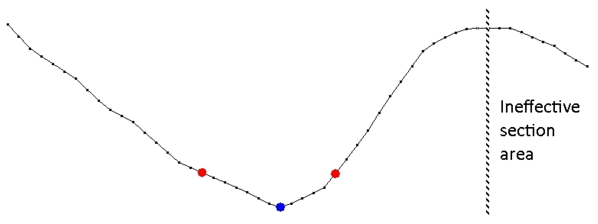
2.4.6. Removal of Ineffective Areas

As previously explained, the overbank curves are being formed with a constant offset from the bank curves. This means that the length of the floodplains of the cross-sections is considered constant regardless of the underlying morphology. Occasionally, the outer part of the floodplain is such that no flow can take place inside it. In this case, this part is ineffective since it cannot contribute to the conveyance of the cross-section (i.e., cannot undertake part of the water discharged) and thus can be removed/ignored. Figure 30 shows a typical example, in which a hump lies at the right side, but its ridge is not located at the edge. The points after the ridge have descending elevations; therefore, no channel is formed. This area cannot convey any water and therefore can be removed/ignored.

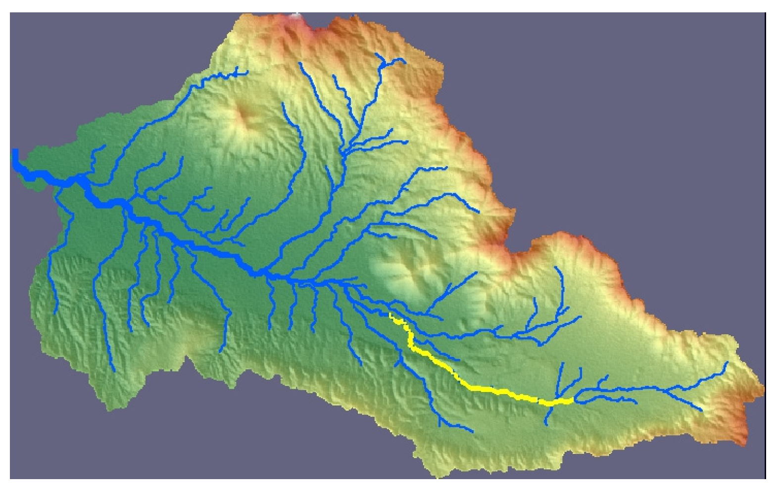
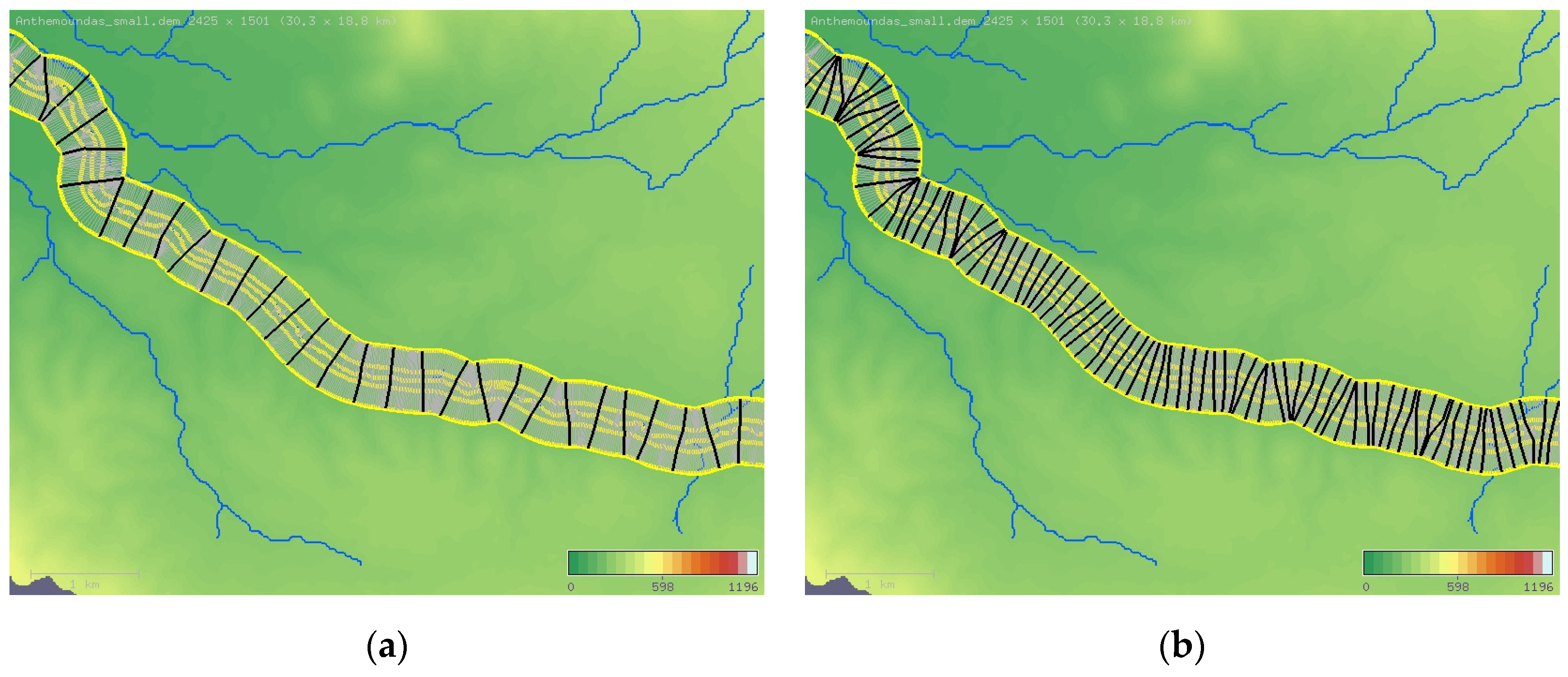
2.5. Selection of the Cross-Sections

As mentioned before, the stream curve (i.e., curve C) consists of a series of successive points c₁, c₂, …, c_n with coordinates Xi, Yi. The procedure described in the previous paragraphs takes place for each cross-section defined for each point of curve C, and each cross-section is marked as valid or invalid. The distance of each cross-section from the beginning of the curve along the stream curve is calculated using the following equation:

$$L_i={{\displaystyle \sum }}_{j=2}^i\sqrt{{\left(x_j-x_{j-1}\right)}^2+{\left(y_j-y_{j-1}\right)}^2}.$$

(13)

From all valid cross-sections, the first one is selected and after that, the next cross-section is the one in which distance from the previously selected one is greater or equal to the specified spacing. The distance between cross-sections i and j is calculated as:

$$Dis{t}_{i-j}=\left|L_i-L_j\right|.$$

(14)

This procedure continues until all cross-sections are examined, and there is no other to be checked. Every time a new cross-section is selected, it is checked against all previous selected cross-sections, and, if it intersects one of them, it is rejected, and the next one is examined. At the end, the cross-sections selected constitute the set that describes the geometry of the stream. The set, depending on the length of the stream and the specified parameters, can contain tens or even thousands of cross-sections. The density of the cross-sections can be altered by changing their spacing. To get the best hydraulic results, it is better to have the cross-sections as close to each other as possible; hence, the spacing should be as small as possible. Figure 31a,b present the projections of the cross-sections (in black) for two different values of spacing, while all other parameters are kept the same. Particularly, in Figure 31a, the spacing is three times as big as the one of Figure 31b. The result is that in the first case 31 cross-sections are defined, while, in the second, 89.

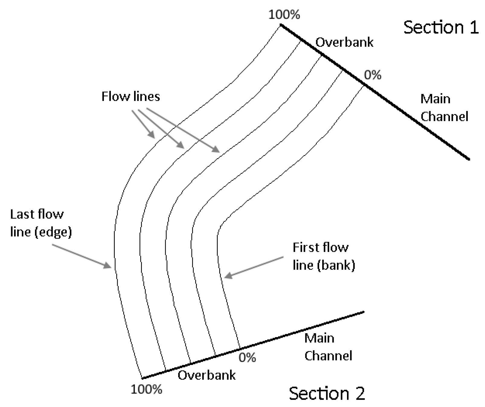
2.6. Calculation of the Distances between the Sections

During the hydraulic calculations, it is necessary to assess the energy losses between the cross-sections, which, among others, depend on their spacing. Three distances are needed for each cross-section: (1) between the main channels; (2) between the left floodplains; and (3) between the right floodplains. Each distance is measured from the respective area of the next downstream cross-section. For the downstream one all three distances are zero. The distance between the main channels is calculated along the stream curve from Equation (14). The distance between the floodplains though, depends on the exact position where the measurement takes place. The anticipated flow lines that start from the floodplain of the first cross-section and end to the floodplain of the second cross-section are approximately parallel to each other. Due to the curvature and the angle between the floodplains, they have different lengths, though. Consequently, this distance depends on the particular flow line examined. It is possible to examine the first flow line, namely the one that coincides with the bank curve (i.e., curves E and F), the last line which coincides with the floodplain’s outer limit (i.e., curves D and G), or any other which lies in the middle. To distinguish among the flow lines, the percentage of the distance (i.e., Overbank Distance %) from the bank (0%) to the edge (100%) can be defined. Ideally, the flow line examined should be the one that divides the water volume into equal parts. The floodplain elevations are usually higher at the edges than at the banks, so the resulting water depth is deeper near the banks (i.e., curves E and F); hence, the water quantity concentrated at the inner part is larger. A representative value for this percentage is 30%, but any value considered the most suitable for the particular stream can be used. This percentage can be defined independently for each floodplain left and right, allowing for better adaption to the morphology of the river. Figure 32 shows the floodplains of two successive cross-sections and the flow lines between them. In this example, as the flow lines move towards the outer part, they get longer.

Although the distance along the selected flow line could be calculated in a similar manner (Equation (13)), this is generally not possible as the particular flow line’s path is not calculated. Assuming that the cross-sections involved are i and j > i and that the calculation takes place for the left floodplain, the distance is calculated applying the following technique: Three distances are calculated: (a) the distance D_i−j along the bank curve; (b) the straight distance D₀ between the banks; and (c) the straight distance D₁₀₀ between the overbanks. The distance along the bank curve is calculated from Equation (15). The straight line distance between the banks (0%) is calculated from Equation (16), while the straight line distance between the overbanks (100%) is calculated from Equation (17):

$$D_{i-j}={{\displaystyle \sum }}_{k=i+1}^j\sqrt{{\left(x_k-x_{k-1}\right)}^2+{\left(y_k-y_{k-1}\right)}^2},$$

(15)

$$D_0=\sqrt{{\left(x{e}_i-x{e}_j\right)}^2+{\left(y{e}_i-y{e}_j\right)}^2},$$

(16)

$$D_{100}=\sqrt{{\left(x{d}_i-x{d}_j\right)}^2+{\left(y{d}_i-y{d}_j\right)}^2}.$$

(17)

Then, the distance DF_P along the required flow line at P% is approximated through linear interpolation according to the following equation:

$$D{F}_P=D_{i-j}+\frac{P}{100}·\left(D_{100}-D_0\right).$$

(18)

3. Results

The algorithm has been tested for various scenarios and DEMs. The DEMs used derived from the SRTM1 project (resolutions of 1” = arc second) and the ALOS PALSAR [32] project (resolutions of 12.5 × 12.5 m). The rivers and streams were extracted using the HYDROLOGY software that can display the DEMs, the hydrographic network, the curves used for the construction of the cross-sections, and the cross-sections themselves. Figure 33 shows part of river Chavrias (colored in yellow), which flows in the northern part of Greece and in particular in central Chalkidiki. This particular part of the river is 1500 m long and flows from northwest to southeast. The elevations of the inverts range from 118 to 140 m. This part was selected because it has great sinuosity and therefore is suitable to check the distribution of the cross-sections in the DEM’s plan view. The area map appears on the left side of Figure 33, while the entire basin of the river appears in the middle of it.

Two different sets were extracted, the first with non-planar and the second with planar cross-sections.

3.1. First Set—Non Planar Cross-Sections

The automatic detection of the banks was deactivated by setting too high values for the two respective parameters (Max Height and Levee Height). This was deliberately done in order to force the bank curves to be formed at a constant distance of 60 m by setting the respective parameter (Max Dist) equal to this value. The Overbank distance was set to 140 m. The restriction for the angle between the cross-sections and the stream path (Min Angle) was set to 75 degrees. The spacing was set to the same value as the resolution, which is 12.5 m. Figure 34a shows the outcome of these parameters. A total of 101 non-planar cross-sections were extracted, and, as it can be seen, they are evenly distributed along the stream. The actual spacing varied from 12.5 to 17.7 m, with a mean value of 14.9 m.

3.2. Second Set—Planar Cross-Sections

The second set was processed with the same spacing (12.5 m) and the same restriction for the angle (parameter Min Angle = 75 degrees). Figure 34b shows the outcome. A total of 59 planar cross-sections (in black) were extracted. This value is 41% less than in the one of the first set. The actual spacing varied from 12.5 to 356.9 m with a mean value of 25.7 m. As it can be seen, there are parts of the stream where no cross-sections could be extracted. The cross-sections that appear in light grey color were rejected because their angle with the stream’s path was less than the specified angle. Figure 35 presents three representative sections of the first set.

Figure 36 presents the flood inundation mapping (FIM) of the first set for three different values of discharge. The display method selected for the DEM is the relief map. The extent of the water appears for the part of the stream that is solved. The color of the water depends on the current depth and appears white for shallow depths, cyan for intermediate depths, and dark blue for the biggest depth of each image. In Figure 36a, the discharge is set to 400 m³/s, and the calculated maximum depth is 4.8 m. In Figure 36b, the discharge is set to 4000 m³/s, and the calculated maximum depth is 11.8 m. In Figure 36c, the discharge is set to 40,000 m³/s, and the calculated maximum depth is 37.2 m. The water level and extent in this figure is such that some of the sections are flooded. The calculation was done directly inside the software HYDROLOGY.

4. Discussion and Conclusions

So far, the extraction of cross sections from DEMs is being done in a manual way in a GIS environment. Pilotti in 2016, presented a methodology where cross-sections could be extracted in an automated way. Unfortunately, following Pilotti’s methodology, the cross-sections are constrained to be planar, a fact that prevents them from being evenly spaced. Furthermore, the cross-sections are extracted with a single friction coefficient neglecting the existence of the overbank areas.

In this paper a new methodology along with a respective Parametric Cross-sections Extraction Algorithm (PCSEA) for the fully automatic extraction of hydraulic cross-sections from Digital Elevation Models (DEMs) are presented. Both the methodology and the algorithm suggested successfully address troublemaking issues not resolved by previous researchers, providing high quality, evenly spaced cross-sections with banks, overbank areas, and separate friction coefficients for each. These cross-sections are non-planar, a property that has two important advantages over the planar cross-sections: (a) it ensures that they are perpendicular to the flow at each subsection, and (b) it allows creation of a much denser sequence, since non planar cross-sections can approach each other closer than their planar counterparts. The idea in which the whole approach is based is to design four curves aside the stream centerline curve from which the cross-sections will be created. The geometric characteristics of these curves ensure that each cross-section will be perpendicular to the flow along its entire span. The points of these curves are the endpoints of each cross-section to be created. The two inner curves reside next to the stream centerline path and consist of the banks of each cross-section. These banks are automatically detected with respect to two different criteria. The other two curves consist of the overbank limits of each cross-section. Some of the cross-sections extracted with this procedure fail to satisfy certain criteria of validity and therefore cannot be used. The sequence of the cross-sections extracted is obtained from the valid ones, and its density depends on the spacing defined.

It was proven that non-planar cross-sections can be evenly distributed even in parts of the stream that present great values of sinuosity, providing a high quality high density sequence. This renders their use a necessity instead of their planar counterparts, which have certain limitations and allows high accuracy results to be produced when they are used in hydraulic simulations. The profile of each cross-section is calculated from the elevations of the DEM with bilinear interpolation and depends on the segment length selected. Sometimes, the shape of the channel bed of rivers in DEMs is affected by limitations of the remote sensing method used for their construction. A new method was developed to improve this shape whenever it appears flat by converting it to parabolic. This results in an increase of the channel’s effective area and of its conveyance. Another feature provided is the automatic definition of levees. Levees restrict the flow of water in secondary channels of the cross-section.

The algorithm developed is fully parametric and it can be repetitively applied until the desirable result is achieved, simply by altering any of the specified parameters. If the algorithm is combined with visual presentation of the results with appropriate software that provides graphic capabilities, it will provide instant feedback to confirm or modify the design parameters at the time of extraction. The cross-sections extracted are geometrically complete, and, if the roughness coefficients (Manning’s coefficients) and the coefficients for contraction and expansion are defined, they can be exported for use with hydraulic simulation software, such as ARHA or HEC-RAS.

This package is considered a valuable tool for its user (i.e., engineer/decision maker), as it quickly provides preliminary reliable conclusions for any case study area without requiring any former experience or training. These conclusions can lead to a better aimed choice of positions in which field surveys will be conducted. If high resolution hydrologically corrected DEMs become publicly available in the future, this technique may allow full substitution of the field surveys, thus enabling cost reduction and the ability to conduct more flood or hydrodynamic simulations and better estimate or predict the consequences of this kind of natural phenomena.

References

- Bures, L.L.; Roub, R.; Sychová, P.; Gdulova, K.; Doubalova, J. Comparison of bathymetric data sources used in hydraulic modeling of floods. J. Flood Risk Manag. 2018, 12. [Google Scholar] [CrossRef]
- Domeneghetti, A. On the use of SRTM and altimetry data for flood modeling in datasparse regions. Water Resour. Res. 2016, 52, 2901–2907. [Google Scholar] [CrossRef]
- NASA. Shuttle Radar Topography Mission (SRTM); NASA: Washington, DC, USA, 2000. [Google Scholar]
- Charlton, M.E.; Large, A.R.G.; Fuller, I.C. Application of airborne LiDAR in river environments: The River Coquet, Northumberland, UK. Earth Surf. Process. Landf. 2003, 28, 299–306. [Google Scholar] [CrossRef]
- Ludwig, R.; Schneider, P. Validation of digital elevation models from SRTM X-SAR for applications in hydrologic modeling. ISPRS J. Photogramm. Remote Sens. 2006, 60, 339–358. [Google Scholar] [CrossRef]
- Walker, J.P.; Willgoose, G.R. On the effect of digital elevation model accuracy on hydrology and geomorphology. Water Resour. Res. 1999, 35, 2259–2268. [Google Scholar] [CrossRef]
- Yin, Z.Y.; Wang, X. A cross-scale comparison of drainage basin characteristics derived from digital elevation models. Earth Surf. Process. Landf. 1999, 24, 557–562. [Google Scholar] [CrossRef]
- Casas, A.; Benito, G.; Thorndycraft, V.R.; Rico, M. The topographic data source of digital terrain models as a key element in the accuracy of hydraulic flood modeling. Earth Surf. Process. Landf. 2006, 31, 444–456. [Google Scholar] [CrossRef]
- Schumann, G.; Matgen, P.; Cutler, M.E.J.; Black, A.; Hoffmann, L.; Pfister, L. Comparison of remotely sensed water stages from LiDAR, topographic contours and SRTM. ISPRS J. Photogramm. Remote Sens. 2008, 63, 283–296. [Google Scholar] [CrossRef]
- Ali, A.M.; Solomatine, D.P.; Di Baldassarre, G. Assessing the impact of different sources of topographic data on 1-D hydraulic modeling of floods. Hydrol. Earth Syst. Sci. 2015, 19, 631. [Google Scholar] [CrossRef]
- Mersel, M.K.; Smith, L.C.; Andreadis, K.M.; Durand, M.T. Estimation of river depth from remotely sensed hydraulic relationships. Water Resour. Res. 2013, 49, 3165–3177. [Google Scholar] [CrossRef]
- Yan, K.; Di Baldassarre, G.; Solomatine, D.P. Exploring the potential of SRTM topographic data for flood inundation under uncertainty. J. Hydroinform. 2013, 15, 849–861. [Google Scholar] [CrossRef]
- Andersson, E.; Hietala, S. Application of a New Method to Improve River Cross-Sections Derived from Satellite Images; Degree Project in Technology: Stockholm, Sweden, 2018. [Google Scholar]
- Pramanik, N.; Panda, R.K.; Sen, D. One dimensional hydrodynamic modeling of river flow using DEM extracted river cross-sections. Water Resour. Manag. 2010, 24, 835–852. [Google Scholar] [CrossRef]
- Hydrologic Engineering Center. HEC-RAS River Analysis System; Version 5.0.7.; Hydrologic Engineering Center: Davis, CA, USA, 2019. [Google Scholar]
- Environmental Systems Research Institute (ESRI). ArcGIS Desktop 10.8; Environmental Systems Research Institute (ESRI): Redlands, CA, USA, 2020. [Google Scholar]
- Hydrologic Engineering Center. HEC-RAS 2D Modeling User’s manual; Hydrologic Engineering Center: Davis, CA, USA, 1991. [Google Scholar]
- Samuels, P.G. Cross-section location in one-dimensional models. In Proceedings of International Conference on River Flood Hydraulics; White, W.R., Ed.; John Wiley: Chichester, UK, 1990; pp. 339–350. [Google Scholar]
- Castellarin, A.; Di Baldassarre, G.; Bates, P.D.; Brath, A. Optimal cross-sectional spacing in Preissmann scheme 1D hydrodynamic models. J. Hydraul. Eng. 2009, 135, 96–105. [Google Scholar] [CrossRef]
- Gichamo, T.Z.; Popescu, I.; Jonoski, A.; Solomatine, D. River cross-section extraction from the ASTER global DEM for flood modeling. Environ. Modeling Softw. 2012, 31, 37–46. [Google Scholar] [CrossRef]
- ASTER GDEM. ASTER Global DEM Validation Summary Report. METI/ERSDAC, NASA/LPDAAC, USGS/EROS; 2009. Available online: https://asterweb.jpl.nasa.gov/gdem.asp (accessed on 5 August 2019).
- Pilotti, M. Extraction of cross-sections from digital elevation model for one-dimensional dam-break wave propagation in mountain valleys. Water Resour. Res. 2016, 52, 52–68. [Google Scholar] [CrossRef]
- Petikas, I.; Keramaris, E.; Kanakoudis, V. Calculation of Multiple Critical Depths in Open Channels Using an Adaptive Cubic Polynomials Algorithm. Water 2020, 12, 799. [Google Scholar] [CrossRef]
- Petikas, I. Development and Application of Innovative Methodologies, Software and Algorithms (ACPA, BECPA, ARHA, HYDROLOGY) for the Precise Calculation of Hydraulic Flow Characteristics in the Design of Flood Mitigation Works. Ph.D. Thesis, Civil Engineering Department, University of Thessaly, Thessaly, Greece, 2020. (in progress). [Google Scholar]
- Fairfield, J.; Leymarie, P. Drainage Networks from Grid Digital Elevation Models. Water Resour. Res. 1991, 27, 709–771. [Google Scholar] [CrossRef]
- Tarboton, D.G. A new method for the determination of flow directions and upslope areas in grid digital elevation models. Water Resour. Res. 1997, 33, 309–319. [Google Scholar] [CrossRef]
- Planchon, O.; Darboux, F. A fast, simple and versatile algorithm to fill the depressions of digital elevation models. Catena 2001, 46, 159–176. [Google Scholar] [CrossRef]
- O’Callaghan, J.F.; Mark, D.M. The extraction of drainage networks from digital elevation data. Comput. Vis. Graph. Image Process. 1984, 28, 323–344. [Google Scholar] [CrossRef]
- Jenson, S.K.; Domingue, J.O. Extracting topographic structure from digital elevation data for geographic information system analysis. Photogramm. Eng. Remote Sens. 1988, 54, 1593–1600. [Google Scholar]
- Tarboton, D.; Ames, D.P. Advances in the Mapping of Flow Networks from Digital Elevation Data. In Proceedings of the World Water and Environmental Resources Congress, Orlando, FL, USA, 20–24 May 2001; pp. 1–10. [Google Scholar]
- Smith, M.J.; Clark, C.D. Methods for the visualization of digital elevation models for landform mapping. Earth Surf. Process. Landf. 2005, 30, 885–900. [Google Scholar] [CrossRef]
- JAXA. Advanced Land Observing Satellite Phased Array Type L-Band Synthetic Aperture Radar (ALOS PALSAR); JAXA: Tokyo, Japan, 2006. [Google Scholar]
Publisher’s Note: MDPI stays neutral with regard to jurisdictional claims in published maps and institutional affiliations. |
© 2020 by the authors. Licensee MDPI, Basel, Switzerland. This article is an open access article distributed under the terms and conditions of the Creative Commons Attribution (CC BY) license (http://creativecommons.org/licenses/by/4.0/).
Share and Cite
Petikas, I.; Keramaris, E.; Kanakoudis, V. A Novel Method for the Automatic Extraction of Quality Non-Planar River Cross-Sections from Digital Elevation Models. Water 2020, 12, 3553. https://doi.org/10.3390/w12123553
Petikas I, Keramaris E, Kanakoudis V. A Novel Method for the Automatic Extraction of Quality Non-Planar River Cross-Sections from Digital Elevation Models. Water. 2020; 12(12):3553. https://doi.org/10.3390/w12123553
Chicago/Turabian StylePetikas, Ioannis, Evangelos Keramaris, and Vasilis Kanakoudis. 2020. "A Novel Method for the Automatic Extraction of Quality Non-Planar River Cross-Sections from Digital Elevation Models" Water 12, no. 12: 3553. https://doi.org/10.3390/w12123553
APA StylePetikas, I., Keramaris, E., & Kanakoudis, V. (2020). A Novel Method for the Automatic Extraction of Quality Non-Planar River Cross-Sections from Digital Elevation Models. Water, 12(12), 3553. https://doi.org/10.3390/w12123553