Figure 1.
The Colorado River near Yuma, AZ provides an example of meander bends (photograph taken 4 January 2007).
Figure 1.
The Colorado River near Yuma, AZ provides an example of meander bends (photograph taken 4 January 2007).
Figure 2.
Typical river channel cross section with super elevation around a meander bend that causes a pressure imbalance and induces a secondary flow current. The arrows denote the direction of downstream flow on the water surface (light blue shading) and secondary circulation in cross section (medium blue shading).
Figure 3.
Planform phase lag definition sketch.
Figure 3.
Planform phase lag definition sketch.
Figure 4.
Twelve model simulation sets spanned three orders of magnitude of discharge (2.83, 28.3, 283, and 2832 m
3/s), four orders of magnitude of longitudinal valley slope (7.11 × 10
−6 to 2.69 × 10
−2), and an order of magnitude in medium sediment grain size (0.125 to 4 m) (modified from Chang [
50]).
Figure 5.
Example meandering river channel alignment, generated using a sine-generated curve, for Simulation Set 5 with a sinuosity of 2.75 and five consecutive curves. The upstream and downstream segments of the synthetic channel are straight and 15 channel widths long.
Figure 5.
Example meandering river channel alignment, generated using a sine-generated curve, for Simulation Set 5 with a sinuosity of 2.75 and five consecutive curves. The upstream and downstream segments of the synthetic channel are straight and 15 channel widths long.
Figure 6.
A series of meandering channel alignments (from Simulation Set 6, with three consecutive bends) are compared for a range of sinuosity from 1.1 to 3.0.
Figure 6.
A series of meandering channel alignments (from Simulation Set 6, with three consecutive bends) are compared for a range of sinuosity from 1.1 to 3.0.
Figure 7.
Photograph looking upstream at the Colorado State University (CSU) physical model with flow through two channel curves.
Figure 7.
Photograph looking upstream at the Colorado State University (CSU) physical model with flow through two channel curves.
Figure 8.
Plan-view of the open channel, physical model by Yen [
58]. The positions of cross sections where velocity profiles were measured are identified as S0, CIIO, π/16, π/8, and π/4.
Figure 8.
Plan-view of the open channel, physical model by Yen [
58]. The positions of cross sections where velocity profiles were measured are identified as S0, CIIO, π/16, π/8, and π/4.
Figure 9.
Comparison of simulated and measured velocity profile at cross-section S0 at position −0.461 B.
Figure 9.
Comparison of simulated and measured velocity profile at cross-section S0 at position −0.461 B.
Figure 10.
Comparison of simulated and measured velocity profile at cross-section S0 at position −0.307 B.
Figure 10.
Comparison of simulated and measured velocity profile at cross-section S0 at position −0.307 B.
Figure 11.
Comparison of simulated and measured velocity profile at cross-section S0 at position 0.00 B.
Figure 11.
Comparison of simulated and measured velocity profile at cross-section S0 at position 0.00 B.
Figure 12.
Comparison of simulated and measured velocity profile at cross-section S0 at position +0.307 B.
Figure 12.
Comparison of simulated and measured velocity profile at cross-section S0 at position +0.307 B.
Figure 13.
Comparison of simulated and measured velocity profile at cross-section S0 at position +0.461 B.
Figure 13.
Comparison of simulated and measured velocity profile at cross-section S0 at position +0.461 B.
Figure 14.
Patterns of dimensionless boundary shear stress simulated using the fine three-dimensional (3D) model mesh.
Figure 14.
Patterns of dimensionless boundary shear stress simulated using the fine three-dimensional (3D) model mesh.
Figure 15.
Comparison of simulated and measured shear stress for cross-section CIIO (upstream entrance to second channel curve). The channel cross section is also plotted along with the location of greatest velocity (within 90% percent of maximum velocity).
Figure 15.
Comparison of simulated and measured shear stress for cross-section CIIO (upstream entrance to second channel curve). The channel cross section is also plotted along with the location of greatest velocity (within 90% percent of maximum velocity).
Figure 16.
Comparison of simulated and measured shear stress for cross-section π/16 (11.25° through the second channel curve). The channel cross section is also plotted along with the location of greatest velocity (within 90% of maximum velocity).
Figure 16.
Comparison of simulated and measured shear stress for cross-section π/16 (11.25° through the second channel curve). The channel cross section is also plotted along with the location of greatest velocity (within 90% of maximum velocity).
Figure 17.
Comparison of simulated and measured shear stress for cross-section π/8 (22.5° through the second channel curve). The channel cross section is also plotted along with the location of greatest velocity (within 90% of maximum velocity).
Figure 17.
Comparison of simulated and measured shear stress for cross-section π/8 (22.5° through the second channel curve). The channel cross section is also plotted along with the location of greatest velocity (within 90% of maximum velocity).
Figure 18.
Comparison of simulated and measured shear stress for cross-section π/4 (45° through the second channel curve). The channel cross section is also plotted along with the location of greatest velocity (within 90% of maximum velocity).
Figure 18.
Comparison of simulated and measured shear stress for cross-section π/4 (45° through the second channel curve). The channel cross section is also plotted along with the location of greatest velocity (within 90% of maximum velocity).
Figure 19.
Comparison of boundary shear stress simulated by the U
2RANS model (
left) and measured from the physical model (
right) [
59].
Figure 19.
Comparison of boundary shear stress simulated by the U
2RANS model (
left) and measured from the physical model (
right) [
59].
Figure 20.
Simulated bottom shear stress long the centerline of a straight trapezoidal channel from Simulation Set 6 (bottom width of 20.3 m).
Figure 20.
Simulated bottom shear stress long the centerline of a straight trapezoidal channel from Simulation Set 6 (bottom width of 20.3 m).
Figure 21.
Relative discharge on the left and right sides of the channel centerline through five consecutive meander bends.
Figure 21.
Relative discharge on the left and right sides of the channel centerline through five consecutive meander bends.
Figure 22.
Example of simulated shear stress, and region of highest velocity, at a cross section from the fourth meander bends of Simulation Set 4 with a sinuosity of 2.00. A mesh size of 1142 × 31 × 28 (991,256 mesh cells) was used in the simulation.
Figure 22.
Example of simulated shear stress, and region of highest velocity, at a cross section from the fourth meander bends of Simulation Set 4 with a sinuosity of 2.00. A mesh size of 1142 × 31 × 28 (991,256 mesh cells) was used in the simulation.
Figure 23.
Plan view of the structured 2D model mesh domain for Simulation Set 5 with a sinuosity of 2.75.
Figure 23.
Plan view of the structured 2D model mesh domain for Simulation Set 5 with a sinuosity of 2.75.
Figure 24.
Close-up plan view of the structured two-dimensional (2D) model mesh for Simulation Set 5 with a sinuosity of 2.75.
Figure 24.
Close-up plan view of the structured two-dimensional (2D) model mesh for Simulation Set 5 with a sinuosity of 2.75.
Figure 25.
Water surface elevation contours from the 2D model results for Simulation Set 5 with a sinuosity of 2.75.
Figure 25.
Water surface elevation contours from the 2D model results for Simulation Set 5 with a sinuosity of 2.75.
Figure 26.
Concept of the 3D structured mesh is presented for the right half of the cross section.
Figure 26.
Concept of the 3D structured mesh is presented for the right half of the cross section.
Figure 27.
Simulated 3D velocity contours at the water surface for Simulation Set 5 with a sinuosity of 2.75.
Figure 27.
Simulated 3D velocity contours at the water surface for Simulation Set 5 with a sinuosity of 2.75.
Figure 28.
Close-up 3D view of cross-sectional slices of velocity contours.
Figure 28.
Close-up 3D view of cross-sectional slices of velocity contours.
Figure 29.
Simulated thread of maximum velocity for Simulation Set 5 with a sinuosity of 2.75.
Figure 29.
Simulated thread of maximum velocity for Simulation Set 5 with a sinuosity of 2.75.
Figure 30.
Channel bottom shear stress contours for Simulation Set 5 with a sinuosity of 2.75.
Figure 30.
Channel bottom shear stress contours for Simulation Set 5 with a sinuosity of 2.75.
Figure 31.
Dimensionless shear stress along the channel centerline, left and right banks for Simulation Set 5 with a sinuosity of 2.75.
Figure 31.
Dimensionless shear stress along the channel centerline, left and right banks for Simulation Set 5 with a sinuosity of 2.75.
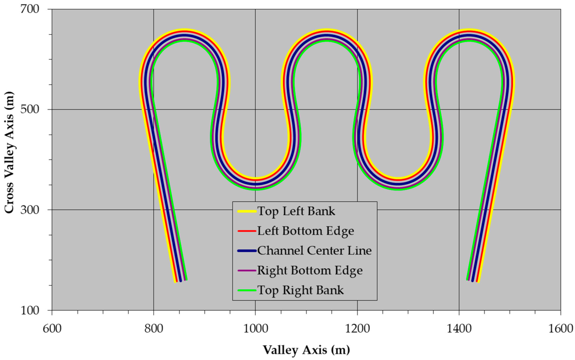
Figure 32.
Plan-view alignment and positions of selected cross-sections 112, 702, 810, and 950 for Simulation set 5 with a sinuosity of 2.75.
Figure 32.
Plan-view alignment and positions of selected cross-sections 112, 702, 810, and 950 for Simulation set 5 with a sinuosity of 2.75.
Figure 33.
Cross-section 112 (upstream straight reach) lateral distribution of shear stress and zone where velocity is at least 90 percent of the maximum velocity.
Figure 33.
Cross-section 112 (upstream straight reach) lateral distribution of shear stress and zone where velocity is at least 90 percent of the maximum velocity.
Figure 34.
Cross-section 702 (3rd meander bend) lateral distribution of shear stress and zone where velocity is at least 90 percent of the maximum velocity.
Figure 34.
Cross-section 702 (3rd meander bend) lateral distribution of shear stress and zone where velocity is at least 90 percent of the maximum velocity.
Figure 35.
Cross-section 810 (3rd meander bend) lateral distribution of shear stress and zone where velocity is at least 90 percent of the maximum velocity.
Figure 35.
Cross-section 810 (3rd meander bend) lateral distribution of shear stress and zone where velocity is at least 90 percent of the maximum velocity.
Figure 36.
Cross-section 950 (3rd meander bend) lateral distribution of shear stress and zone where velocity is at least 90 percent of the maximum velocity.
Figure 36.
Cross-section 950 (3rd meander bend) lateral distribution of shear stress and zone where velocity is at least 90 percent of the maximum velocity.
Figure 37.
Vertical streamwise velocity profiles at Cross-section 112 (upstream straight reach) for Simulation Set 5 with a sinuosity of 2.75.
Figure 37.
Vertical streamwise velocity profiles at Cross-section 112 (upstream straight reach) for Simulation Set 5 with a sinuosity of 2.75.
Figure 38.
Vertical streamwise velocity profiles at Cross-section 702 (3rd meander bend) for Simulation Set 5 with a sinuosity of 2.75.
Figure 38.
Vertical streamwise velocity profiles at Cross-section 702 (3rd meander bend) for Simulation Set 5 with a sinuosity of 2.75.
Figure 39.
Vertical streamwise velocity profiles at Cross-section 810 (3rd meander bend) for Simulation Set 5 with a sinuosity of 2.75.
Figure 39.
Vertical streamwise velocity profiles at Cross-section 810 (3rd meander bend) for Simulation Set 5 with a sinuosity of 2.75.
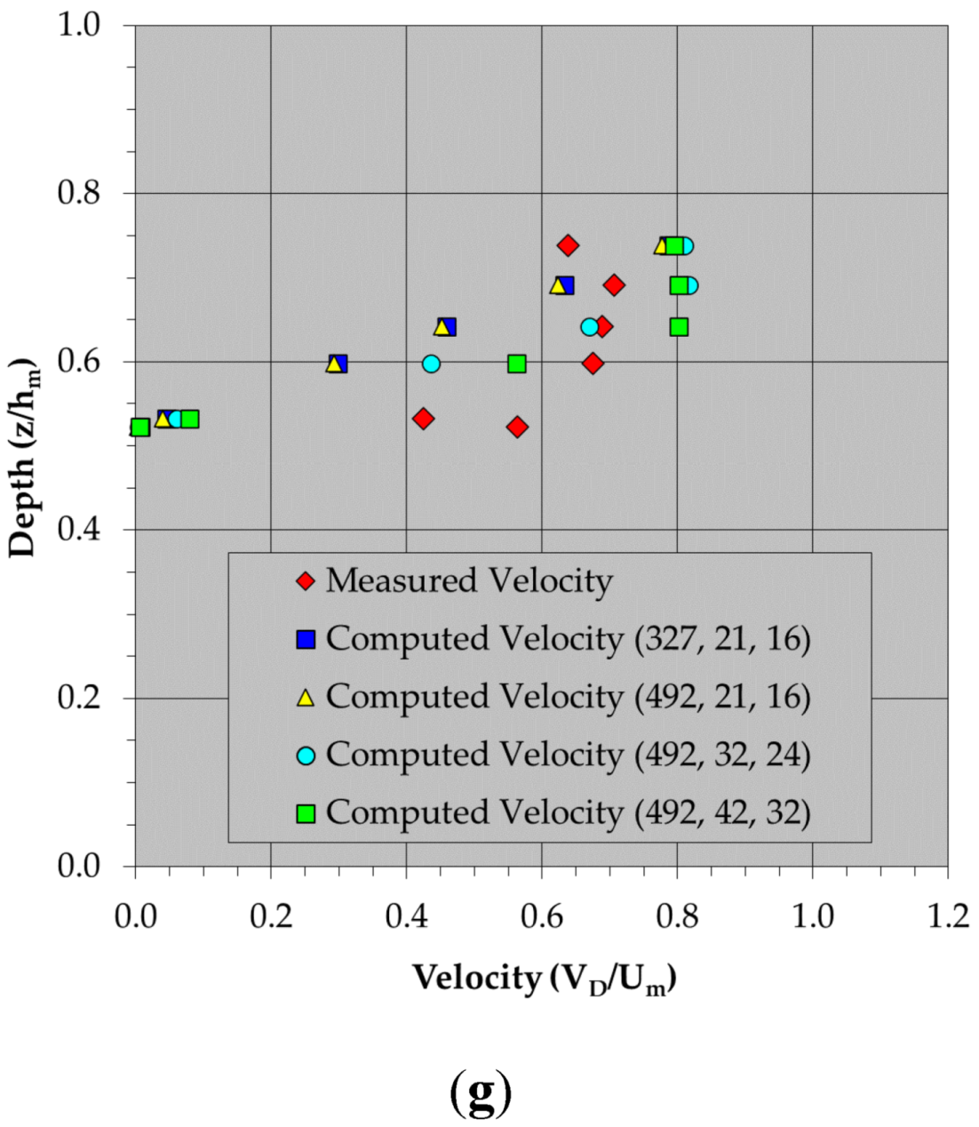
Figure 40.
Vertical streamwise velocity profiles at Cross-section 950 (4th meander bend) for Simulation Set 5 with a sinuosity of 2.75.
Figure 40.
Vertical streamwise velocity profiles at Cross-section 950 (4th meander bend) for Simulation Set 5 with a sinuosity of 2.75.
Figure 41.
Dimensionless shear stress along the channel centerline, left and right banks for Simulation Set 7 with a sinuosity of 2.00 and a width/depth ratio of 7.3.
Figure 41.
Dimensionless shear stress along the channel centerline, left and right banks for Simulation Set 7 with a sinuosity of 2.00 and a width/depth ratio of 7.3.
Figure 42.
Dimensionless shear stress along the channel centerline, left and right banks for Simulation Set 8 with a sinuosity of 2.00 and a width/depth ratio of 9.1.
Figure 42.
Dimensionless shear stress along the channel centerline, left and right banks for Simulation Set 8 with a sinuosity of 2.00 and a width/depth ratio of 9.1.
Figure 43.
Dimensionless shear stress along the channel centerline, left and right banks for Simulation Set 9 with a sinuosity of 2.00 and a width/depth ratio of 35.6.
Figure 43.
Dimensionless shear stress along the channel centerline, left and right banks for Simulation Set 9 with a sinuosity of 2.00 and a width/depth ratio of 35.6.
Figure 44.
Minimum and maximum shear stresses (along the left and right meandering channel banks for Simulation Sets 4–9) versus channel sinuosity.
Figure 44.
Minimum and maximum shear stresses (along the left and right meandering channel banks for Simulation Sets 4–9) versus channel sinuosity.
Figure 45.
Correlations, using 6 simulations sets, between the maximum dimensionless near-bank shear stress and the ratio of channel top width to minimum radius of curvature.
Figure 45.
Correlations, using 6 simulations sets, between the maximum dimensionless near-bank shear stress and the ratio of channel top width to minimum radius of curvature.
Figure 46.
Residuals from 6 simulation sets between the maximum shear stress, computed by Equation (17), and the maximum shear stress simulated by the 3D model versus the channel width/depth ratio.
Figure 46.
Residuals from 6 simulation sets between the maximum shear stress, computed by Equation (17), and the maximum shear stress simulated by the 3D model versus the channel width/depth ratio.
Figure 47.
Correlation of dimensionless shear stress phase lag and channel sinuosity using data from all 6 simulation sets.
Figure 47.
Correlation of dimensionless shear stress phase lag and channel sinuosity using data from all 6 simulation sets.
Figure 48.
Correlations, using all 12 simulations sets, between the maximum dimensionless near-bank shear stress and the ratio of channel top width to minimum radius of curvature.
Figure 48.
Correlations, using all 12 simulations sets, between the maximum dimensionless near-bank shear stress and the ratio of channel top width to minimum radius of curvature.
Figure 49.
Residuals from all 12 simulation sets between the maximum shear stress, computed by Equation (17), and the maximum shear stress simulated by the 3D model versus the channel width/depth ratio.
Figure 49.
Residuals from all 12 simulation sets between the maximum shear stress, computed by Equation (17), and the maximum shear stress simulated by the 3D model versus the channel width/depth ratio.
Figure 50.
Comparison of maximum dimensionless near-bank shear stresses (computed by Equation (23)) and simulated by the 3D model.
Figure 50.
Comparison of maximum dimensionless near-bank shear stresses (computed by Equation (23)) and simulated by the 3D model.
Figure 51.
Correlation of dimensionless shear stress phase lag and channel sinuosity using data from all 12 simulation sets.
Figure 51.
Correlation of dimensionless shear stress phase lag and channel sinuosity using data from all 12 simulation sets.
Figure 52.
Comparison of shear stress phase lags computed by Equations (24)–(26) with phase lags simulated by the 3D model.
Figure 52.
Comparison of shear stress phase lags computed by Equations (24)–(26) with phase lags simulated by the 3D model.
Table 1.
Numerical model simulation sets.
Table 1.
Numerical model simulation sets.
| Simulation Set | Discharge (m3/s) | Valley Slope | Median Sediment Grain Size (mm) | Region |
|---|
| 1 | 2.832 | 6.820 × 10⁻⁴ | 1 | 1 |
| 2 | 2.832 | 6.178 × 10⁻³ | 2 | 1 |
| 3 | 2.832 | 2.693 × 10⁻² | 4 | 3 |
| 4 | 28.32 | 1.490 × 10⁻⁴ | 0.5 | 1 |
| 5 | 28.32 | 1.231 × 10⁻³ | 1 | 1 |
| 6 | 28.32 | 5.885 × 10⁻³ | 2 | 3 |
| 7 | 283.2 | 3.257 × 10⁻⁵ | 0.25 | 1 |
| 8 | 283.2 | 2.454 × 10⁻⁴ | 0.5 | 1 |
| 9 | 283.2 | 1.286 × 10⁻³ | 1 | 3 |
| 10 | 2832 | 7.115 × 10⁻⁶ | 0.125 | 1 |
| 11 | 2832 | 4.890 × 10⁻⁵ | 0.25 | 1 |
| 12 | 2832 | 2.811 × 10⁻⁴ | 0.5 | 3 |
Table 2.
Channel dimensions and hydraulic properties of the physical model reported by Yen [
58].
Table 2.
Channel dimensions and hydraulic properties of the physical model reported by Yen [
58].
| Channel bottom width | 1.829 m |
| Average channel depth | 0.156 m |
| Average wetted top width | 2.141 m |
| Width-depth ratio | 13.7 |
| Upstream straight reach length | 2.134 m |
| Upstream curve radius at centerline | 8.535 m |
| Middle straight reach length | 4.267 m |
| Downstream curve radius at centerline | 8.535 m |
| Downstream straight reach length | 2.134 m |
| Longitudinal channel slope | 0.00072 |
| Discharge | 0.214 m3/s |
| Mean velocity | 0.692 m/s |
| Froude number | 0.56 |
| Reynolds number | 1.14 × 10⁵ |
Table 3.
CSU physical model dimensions.
Table 3.
CSU physical model dimensions.
| Channel Segment | Channel Length (L) (m) | Channel Top Width (T) (m) | Channel Depth (D) (m) | Length/Width (L/T) | Width/Depth (T/D) |
|---|
| Upstream bend | 25.8 | 4.57 | 0.24 | 5.6 | 19.0 |
| Straight transition | 6.5 | 4.57 | 0.31 | 1.4 | 14.7 |
| Downstream bend | 25.6 | 3.7 | 0.31 | 6.9 | 11.9 |
Table 4.
Finest numerical model mesh size used to simulate the flow through the CSU physical model (i, j, and k were the model mesh sizes in the longitudinal, transverse, and vertical dimensions, respectively; L, T, and D were the channel dimensions of length, top width, and depth, respectively).
Table 4.
Finest numerical model mesh size used to simulate the flow through the CSU physical model (i, j, and k were the model mesh sizes in the longitudinal, transverse, and vertical dimensions, respectively; L, T, and D were the channel dimensions of length, top width, and depth, respectively).
| Channel Segment | i | j | k | | | |
|---|
| Straight entrance | 176 | 32 | 24 | 13.4 | 1.68 | 457.0 |
| Upstream bend | 75 | 32 | 24 | 13.3 | 1.68 | 457.0 |
| Straight transition | 20 | 32 | 24 | 14.1 | 2.2 | 353.8 |
| Downstream bend | 75 | 32 | 24 | 10.8 | 2.7 | 286.5 |
| Straight exit | 146 | 32 | 24 | 10.8 | 2.7 | 286.5 |
Table 5.
Validation of empirical equation to predict maximum shear stress for Simulation Sets 1–3 and 10–12. The differences in shear stress (simulated by the 3D model and computed from Equation (18)) were computed for each channel and the minimum and maximum differences are reported here.
Table 5.
Validation of empirical equation to predict maximum shear stress for Simulation Sets 1–3 and 10–12. The differences in shear stress (simulated by the 3D model and computed from Equation (18)) were computed for each channel and the minimum and maximum differences are reported here.
| | Maximum Dimensionless Shear Stress | Shear Stress Difference |
|---|
| | 3D Model Simulations | Empirical
Equation (18) |
|---|
| Minimum | 1.31 | 1.30 | −0.038 |
| Maximum | 1.54 | 1.53 | 0.033 |
| Average | 1.43 | 1.43 | 0.001 |
| RMS Error | | | 0.021 |
Table 6.
Validation of empirical equations to predict phase lag to maximum shear stress for Simulation Sets 1–3 and 10–12. The differences in phase lag (simulated by the 3D model and computed from Equations (19)–(21)) were computed for each channel and the minimum and maximum differences are reported here.
| | Maximum Dimensionless Phase Lag | Phase Lag Difference |
|---|
| | 3D Model Simulations | Empirical
Equations (19)–(21) |
|---|
| Minimum | 0.841 | 0.860 | −0.052 |
| Maximum | 0.986 | 0.956 | 0.075 |
| Average | 0.917 | 0.915 | −0.002 |
| RMS Error | | | 0.027 |

