1. Introduction
Recently, rivers have faced unprecedented challenges in coping with harmful algal blooms (HABs) due to substantial human interventions in natural rivers, including dam construction, agricultural development, and urbanization, which have led to significant changes and the formation of ideal environmental conditions for HABs. Subsequent changes in the water quality of rivers due to algal blooms in water bodies are emerging as a critical problem. For instance, the installation of 15 large weirs after the four major river projects in South Korea has maintained certain water levels which has led to substantially reduced streamflow velocities and nutrient accumulation. Consequently such environmental change has yielded an unprecedented harmful algal bloom (HAB) such as cyanobacteria by promoting eutrophication in these water bodies [
1,
2]. Cyanobacterial algal blooms refer to a phenomenon in which eutrophic lakes or slowly flowing rivers are characterized by the multiplication of algae multiply and its accumulation in large amounts on the surface of the water, which alters the color of the water to green. Flourishing algal blooms have been reported to have adverse effects on the aquatic ecosystem by consuming large amounts of oxygen during decay, thus reducing the dissolved oxygen (DO) in the water. Therefore, algal blooms have a negative effect on water quality and may adversely affect organisms in aquatic ecosystems, such as invertebrates and fish in water bodies. These HABs are recognized as a serious problem for river water quality management because of their effects on aquatic ecosystems [
3] and threat to drinking water systems. In particular, harmful blooms of cyanobacteria can cause serious problems in industrial, domestic, and agricultural water supplies, thus requiring analyses of the causes and countermeasures for HABs for water quality management [
4]. Hence, we must identify the causes of cyanobacterial blooms to protect ecosystems through effective water quality management.
For harmful algal blooms in riverine systems, previous studies have suggested that nutrients, water temperature, and sunlight are the three major triggers for the generation of HABs [
5,
6,
7,
8]. Thus, HABs can be prevented by controlling these three conditions, in which sunlight control is almost impossible. Increasing the water volume and building large dams can help lower the water temperature, but increasing the water volume can reduce the water flow, which can create a favorable environment for the propagation of algae via nutrient accumulation [
9]. In South Korea, after the four major river construction projects, the water volume of the mainstream has increased, but the flow velocity has substantially decreased to almost stagnant flow conditions. The occurrence of algae due to an increased residence time has recently been reported as the most significant problem for the water quality management of rivers [
10].
The vast majority of previous studies have been based on conventional point-based sporadic monitoring of HAB cell numbers with sampling time intervals mostly relying on direct in situ sampling [
11,
12,
13,
14]. The recent advent of remote sensing methods, such as aerial hyperspectral images, has enabled researchers to capture the spatial extent of algal blooms and their evolution at a significant degree of accuracy [
15,
16,
17,
18,
19,
20]. In particular, aerial survey equipment using unmanned aerial vehicles (UAVs) has been widely applied to monitor and investigate HABs in rivers and lakes [
17,
18,
21,
22,
23,
24,
25,
26,
27,
28,
29]. However, we note that despite their high potential, remote sensing approaches are still under development and are currently not widely applied by practitioners, as well having notable limitations in that these approaches are only applicable when algal blooms are already substantial or at least have begun to bloom. In terms of forecasting HABs, various numerical models have been established and received significant improvements, allowing us to investigate how HABs will react and propagate in specific aquatic environments [
18,
21,
30]. However, numerical models are still limited by their ability to sufficiently prove their performance in terms of numerous situations, where the underlying assumptions of numerical modeling are violated and sometimes differ drastically between the modeled and in situ data. In contrast, based only on in situ measurements, the ability to specify HAB-prone regions is of significant interest even before substantial algal blooms develop by evaluating various relevant parameters known to affect HABs, such as nutrients, temperature, flow speed, bathymetry, and turbidity, among others. Such detailed spatial observations of in situ data covering an ample area of large rivers, which can satisfy spatial resolution standards without relying on remote sensing, have been nearly impossible with classic point-based methods or inevitably require expensive instruments, significant funding, and laborious field work; therefore, only limited attempts have been made to date. This is because multiple types of hydrometric and water quality sensors should be intensively utilized. Despite extensive efforts to determine appropriate methods for practical situations, few data-driven approaches have been developed, which have been subsequently regarded as not feasible. Therefore, in the present context, we must develop such methods in a plausible cost-benefit manner.
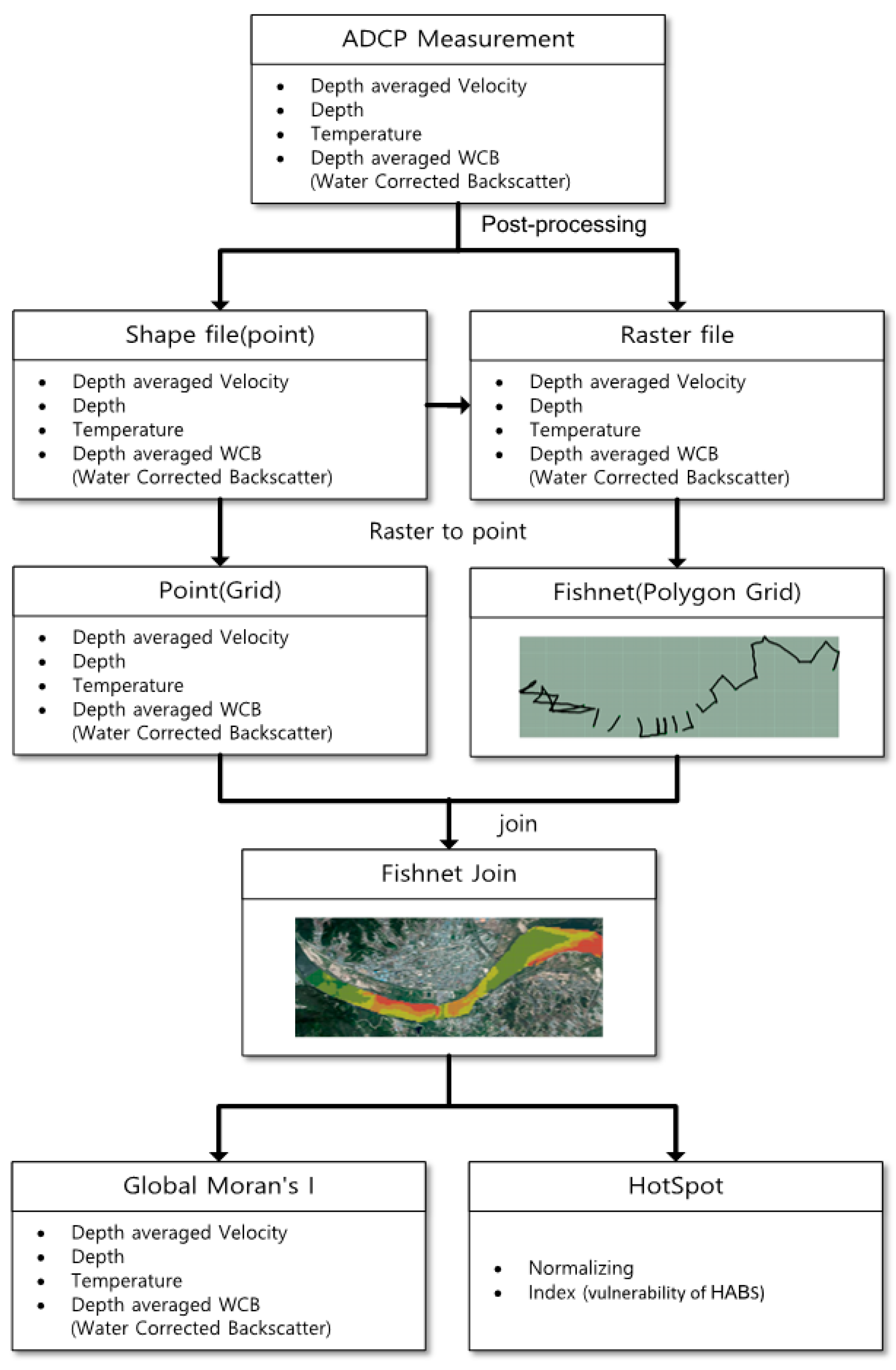
In this study, we propose a practical method to identify HAB-prone regions in riverine environments even before algal blooms develop using only acoustic Doppler current profilers (ADCPs) and applying subsequent machine-learning spatial clustering techniques. ADCPs have been used in riverine observations for several decades, especially for streamflow discharge in its initial stages to establish a classic rating curve and support various hydromorphologic studies. Presently, ADCPs have been well accepted in hydrometric communities, such that that they have become universal in terms of riverine monitoring. In addition to flow velocity measurements using the Doppler effect, we emphasize the fact that ADCPs provide other parameters associated with algal blooms: bathymetry, temperature, and suspended sediment concentrations [
31,
32]. Beside direct measurements by ADCPs, suspended sediment concentrations considered that the intensity of the backscattered ultrasonic signal tends to be proportional to the amount of suspended matter, including sediment and dissolved aquatic materials, and recent such efforts to use ADCPs to spatially map suspended materials have begun to attract attention in hydrometric communities. We hypothesize that these parameters, spatially assessed only by ADCPs (i.e., velocity, bathymetry, temperature, and sediment), can be strongly commensurate with the occurrence of algal blooms, even when certain other relevant parameters, such as the water quality index of nutrients and the sunshine rate, are not available. If even limited parameters, provided only by ADCPs, are capable of deriving HAB-prone regions with a plausible degree of accuracy, with a lack of water quality data, which are usually not spatially available, this approach can have practical significance from a cost-benefit perspective and can be readily used by engineers.
The spatial prediction of HAB-prone regions using the data measured only with an ADCP was performed with “hot-spot” analyses through K-means clustering [
33], as well as the Getis-Ord method [
34,
35]. Before conducting the hot-spot analysis to determine the HAB-prone regions, we must check whether spatially variant in situ ADCP data contain spatial similarities with their neighborhood data (i.e., spatial autocorrelation) or if they are randomly distributed. To yield spatial autocorrelation, Moran’s I concept [
36] was applied in this study. Similarly [
37] quantitatively analyzed the changes in the spatial distribution patterns in marine environments through spatial autocorrelation to understand the spatio-temporal patterns in marine environments. [
38] utilized spatial autocorrelation to relate the spatial correlation of algae observed along a stream in Namdaecheon. Currently, the K-means algorithm has been widely used to predict and classify water quality in rivers and oceans [
39,
40,
41]. As another method of delineating HAB-prone regions, this study also applied a hot-spot analysis based on the Getis-Ord G* method [
34,
35]. Reference [
42] analyzed the spatio-temporal patterns of environmental pollution incidents between 1995 and 2012 using the Getis-Ord G* method.
Collectively, this study took advantage of the full capability of ADCP, such as the flow velocity, depth, temperature, and backscatter, which can explain the physicochemical factors that affect algal blooms. On this basis, the goal of this study is to provide a practical technique to rapidly forecast HAB-prone regions by performing hotspot analysis through the HAB hotspot index, which combines spatial autocorrelation analysis and measurement results based on the K-means cluster analysis and Getis-Ord G* statistic. The proposed method was validated in a study area located at the downstream of the confluence between the Nam and Nakdong river historically known to be susceptible to HABs during the summer season, especially after the construction of the Haman and Hapcheon weirs in 2012, which transformed Nakdong River into a stagnant area capable of storing more water than before. Recently, this area has posed special attention in terms of water quality management by a Chilseo water intake that has taken responsibility as the drinking water supplier to adjacent large cities, such as Daegu and Busan, with a multi-million population, but has suffered severely from annual algal blooms during the summer.
3. Results and Discussion
3.1. ADCP Measurement Results (Flow Velocity, Depth, Temperature, and Backscatter)
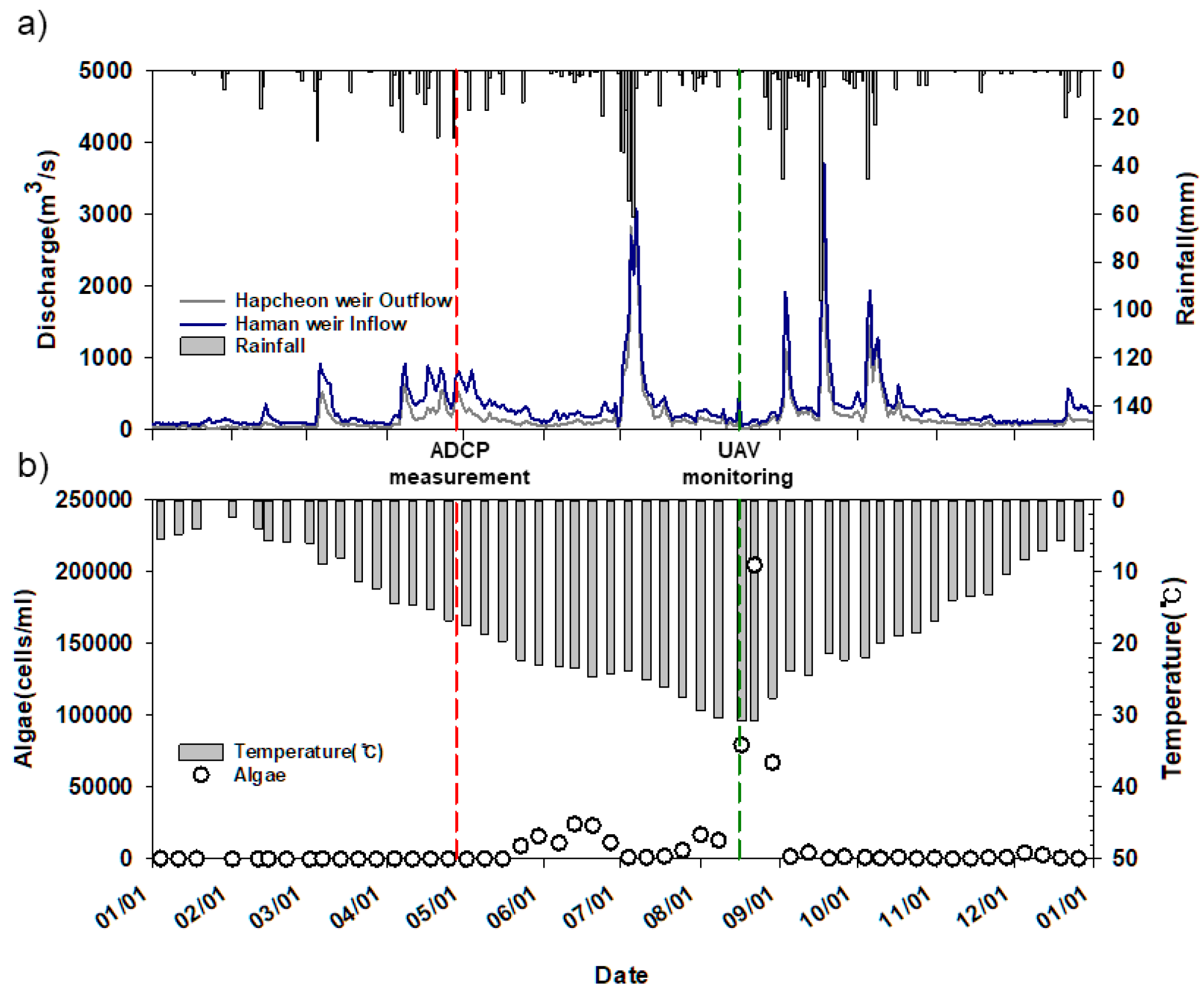
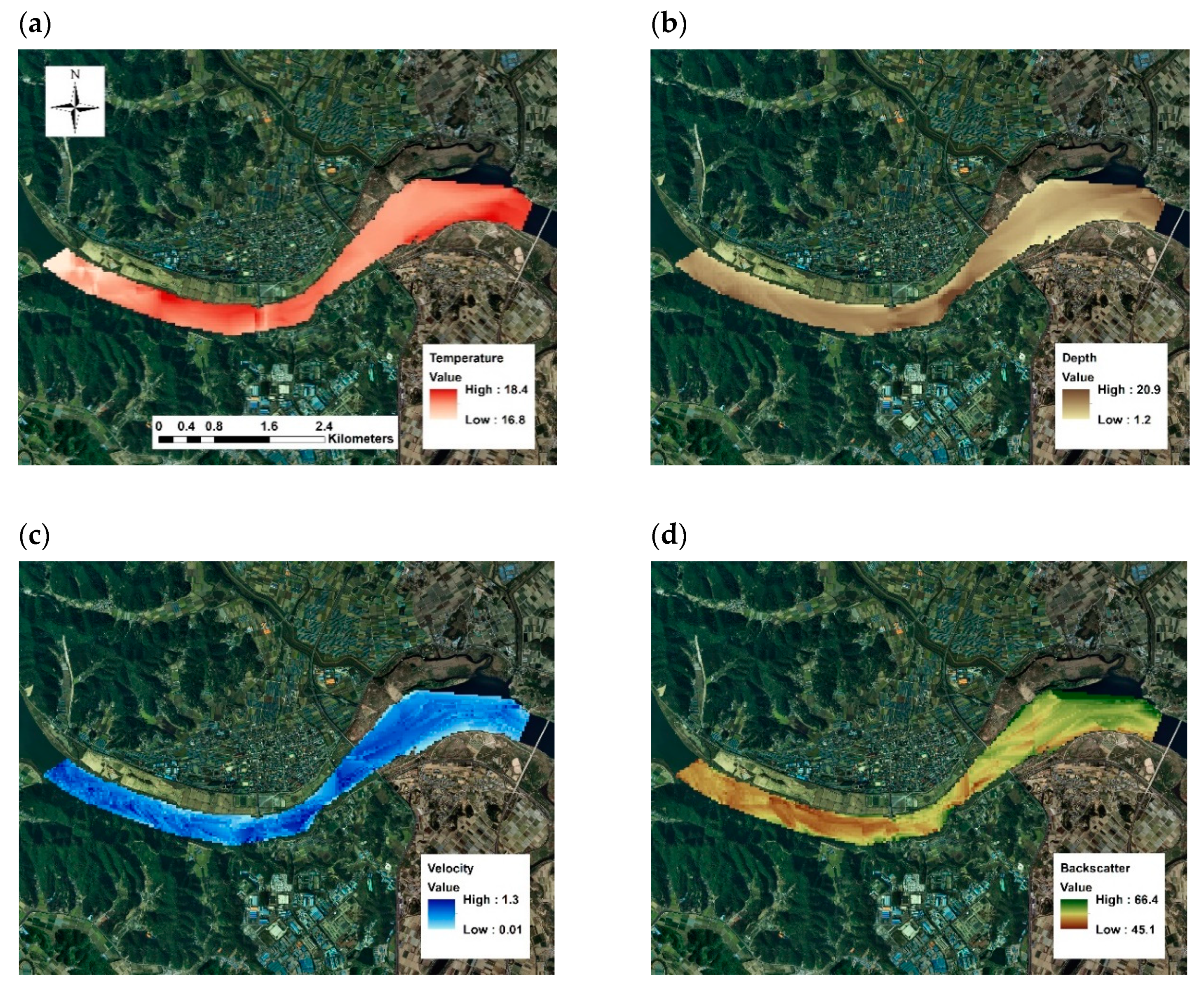
ADCP data were collected, as illustrated in
Figure 1, where spatial interpolation was performed to individually represent the flow velocity, depth, temperature, and backscatter in the form of the maps shown in
Figure 4. The measurements were performed immediately after the rainfall that occurred on 28 April 2016. The temperature was the highest near the left bank, i.e., approximately 1.5 km downstream from the upstream area of the target section, and near the downstream segment of the target section. The water depth was the deepest near the Chilseo water treatment plant while the water depth was shallow near the left bank at the upstream segment of the target section and in the section where the width of the downstream segment widens. Furthermore, the mean flow velocity in the target section was approximately 0.25 m/s, where the flow velocity was low along both banks with shallow bathymetries. The backscatter was the highest at the downstream segment of the target section. The actual measurement results using the ADCP demonstrated notable spatial patterns along the study area and locally clustered regional distinctions. For quantitative evaluation of such a trend, the aforementioned spatial autocorrelation analysis of the target section was performed for each parametric map in terms of the Moran scatter plot with the global Moran’s I and LISA.
3.2. Spatial Autocorrelation
Spatial autocorrelation analysis was conducted to quantitatively determine the existence of spatial correlations inside of each parametric map in
Figure 4. First, the Moran scatter plot was derived for the ADCP parameters in
Figure 5. The Moran scatter plot denotes spatial autocorrelation in an exploratory manor, enabling us to account for how an observed value is similar to its neighborhood observations, where the horizontal axis indicates the observed value and the corresponding vertical axis results in a weighted average within the spatial lag (neighborhood size). Moreover, the slope of regressing the Moran scatter plot indicates the global Moran’s I, which characterizes the overall rate of spatial autocorrelation for the entire dataset with a single value. For example, a value of 1.0 for Moran’s I indicates a perfect correlation with its neighborhood.
Table 1 lists the resulting global Moran’s I for each ADCP parameter. The Moran’s I for temperature, bathymetry, and backscatter indicated very high spatial correlations greater than 0.9, which ultimately led to the fact that these three parameters contain prominent local trends, enabling them to be reasonably grouped for further hotspot analysis. Despite the fact that the velocity was relatively low, i.e., approximately 0.75, noticeably deviated from the other value, the local velocity can change more dynamically compared with the other parameters. However, even the z-score of the velocity reached 136.7, which is similar to the other parameters, indicating that there is still a possibility to formulate clusters with adjacent areas. More specifically, the Moran scatter plot for the bathymetry included certain identifiable outliers that bathymetry can change both locally and substantially. Although the slope is similar between the temperature and backscatter (i.e., sediment), the Moran scatterplot of the backscatter reveals that it was more dispersed than temperature, which indicates that a local uncorrelated region for sediment distribution can exist. Collectively, the global Moran’s analysis of the ADCP parameters outlined a suitable spatial correlation readily useful for further clustering them from the local area to the area toward the HAB-prone region.
In addition to the Global Moran’s I, LISA is a global index for analyzing the spatial autocorrelation with one value [
36]. LISA was performed to analyze the local pattern of spatial autocorrelation in the study area. LISA decomposes the global indicator of Moran’s I into the contribution of each local observation, which, in turn, leads to spatial mapping of the local autocorrelation index. Consequently, LISA can be referred to as the localized Moran’s I, which has been used to assess the influence that individual locations have on the magnitude of the global statistic and identify likely outliers using the Moran scatter plot. In this context, substantiating the trends in a spatial manor is better to ensure local autocorrelation in more detail, rather than Moran’s I and a scatterplot. Among the various degrees used to represent LISA, this study simplified the regions into four categories: HH (high values are surrounded by high values), LL (low values are surrounded by low values), HL (high values are surrounded by low values), and LH (low values are surrounded by high values) This simplified classification was intended to synthetically encapsulate the overall spatial difference affecting the algal blooms and identify their localized presence for the further use of hot-spot analysis.
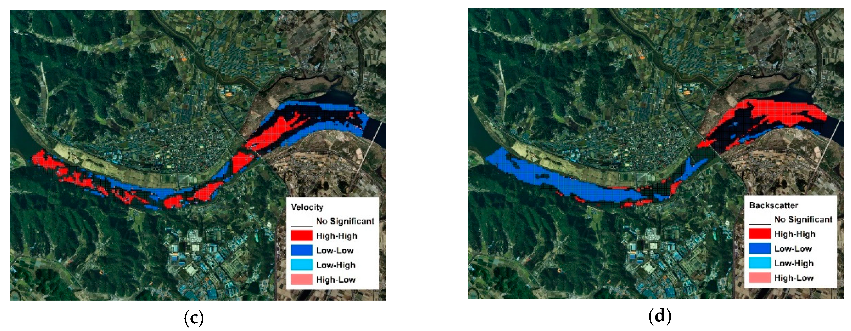
Figure 6 shows the localized spatial autocorrelation driven by the LISA analysis regarding the ADCP measurements, which yields a distinct presence of relatively high and low regions for all four parameters. We note that black-colored vacant areas appeared adjacent to the HH and LL regions, indicating that those regions are not statistically significant and are therefore unable to address local spatial autocorrelation used for further hot-spot analysis.
Physically, this black-colored area may be related to the mixing region induced by tributary flow, especially for the temperature and sediment distribution. For the temperature, a low-temperature area (LL) and a high temperature area (HH) appeared in turn along with the downstream direction. For the morphologic characteristics (i.e., bathymetry), low depth areas (LL) were positioned along the left bank in the initial section while a cluster of LL areas appeared in the most downstream area of the target section. For the flow velocity, LL areas appeared along both banks of the river, similar to the flow velocity distribution of the actual rivers while an HH area formed in the center of the channel. Furthermore, with respect to the backscatter (i.e., suspended matter), the upstream segment of the study area was an LL area while the downstream segment was an HH area. The LISA analysis results for each parameter revealed high temperature, low bathymetry, low velocity, and high backscatter areas with suspended matter in the water body, which can potentially be susceptible to harmful algal blooms, as denoted in Equation(1). This assembled information becomes the underlying cause that plays a crucial role in algal bloom development, from which hot-spots can be more or less interactive.
3.3. Analysis Results of the HAB Hotspots
As mentioned before, this study adapted two methods for hot-spot analysis to identify the HAB-prone regions, i.e., K-means clustering and Getis Ord G*, which yield the coarse classification of HAB-prone regions as hot-spot versus cold-spot areas.
Figure 7 shows the results that can be visually inspected for both approaches collectively using the temperature, depth, flow velocity, and backscatter. These methods ensured that the parameters locally demonstrated spatial autocorrelations, such that they are readily applicable for hot-spot analysis. To expedite the quantitative estimation of the degree of hot spots (i.e., hot or cold spot), the K-means clustering method adapted the number of clusters simply as 2 (i.e., k of the K-means cluster), which enables us to extract the HAB hotspot or not, as represented in
Figure 7a. The results indicate red-colored high areas as hot-spots, commensurate with HAB-prone regions that satisfy high temperature and backscatter, and low bathymetry and velocity based on the required conditions for algae, as described in Equation (1). The subtle texture of hot-spots corresponding to algal blooms formed along both banks of the river, where low bathymetry and velocity were dominant. The right bank in the downstream vicinity of tributary intrusion did not display a high hot-spot (rather a cold-spot), which was mainly attributed to the lower temperature and sediment flow originating from the tributary, i.e., Nam River. In the middle of the downstream segment at the beginning of a meander, however, the effect of the meander and narrowed width increased the flow velocity, yielding a concurrent increase in the bathymetry. Consequently, the hot-spot substantially disappeared in this section. For this reason, our analysis revealed that there are no concerns with respect to algal blooms in this part of the study area. Along with the downstream area where there is a gradual expansion of the river width, the velocity decreased and the bathymetry had a shallower morphology, such that the hot-spot of the HAB-prone region increasingly became more pronounced again.
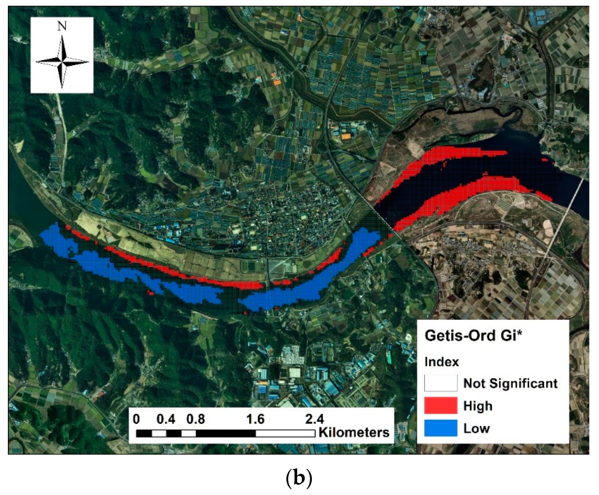
Figure 7b demonstrates the hot-spot analysis using the Getis-Ord G* method, as a second approach, which was, to various degrees, analogous to that of the K-means clustering method shown in
Figure 7a. In comparison with the K-means clustering, the Getis-Ord G* method showed two major differing outcomes. First, the Getis-Ord G* method additionally allocated a black-colored area that is not subject to any high or low category that appeared in the K-means clustering method. In the meantime, the characteristics of this area can be susceptible to both hot and cold regions, suggesting that the algal bloom initiated in the red-colored hot-spot region, such that it more likely pertains to evolution toward this black-colored middle region rather than a cold spot with a blue color. For example, the region immediately downstream of a main bridge (see Nakdong bridge in
Figure 1) was mostly classified as a cold region with blue color, except for a very thin margin of the section of the hot-spot; there was no remarkable difference before and after Nakdong bridge. However, Getis-Ord G* distinctively divided these areas into cold spots before Nakdong bridge, with higher velocity and deeper bathymetry, as well as a black-colored middle region that will be relatively more vulnerable with additional algal blooms, although it is not yet a hot-spot. This result is consistent with the physical characteristics of this area, i.e., streamlining of the locations that accelerated the flow before Nakdong bridge because the meander and narrowed channel width would still maintain the momentum of the stream, particularly in the center of the channel after the bridge. Thus, this centered region is sufficiently mature enough to be characterized as a cold-region, as derived from the K-means clustering method.
Second, in the downstream vicinity of the confluence (significantly upstream of the study area), the Getis-Ord G* method revealed that the right side of the channel can be fully characterized as a cold spot that interacts with the tributary effect. We observed that the texture of the hot-spot in
Figure 7a was not as likely as that shown in
Figure 7b, where the K-means clustering yielded a sporadic and segmented hot-spot along the narrow right side of the channel. This difference may depend on the distance over which the impact of the tributary affected the downstream direction.
3.4. Validation in Conjunction with UAV-Based Photographs
Together with recent advances in UAV monitoring in riverine environments, the monitoring of HABs have become more immediately relevant than other methods, which ensures that the outcomes of this study can be proposed as a comprehensive and quick-and-simple method to ultimately forecast HAB-prone regions. This contemporary type of UAV survey in various riverine environments has become increasingly popular because of its low cost and simple deployment [
47]. Most civil drones are equipped with digital cameras with continuously increasing resolution and positioning accuracy, such that they have become reliable substitutes for conventional expensive aerial photography to visually inspect the spatial trend of HABs over time. The UAV-based monitoring campaign in this study was conducted during August 2016, after HABs had been reported annually in this region every summer, which was a sufficiently long period from the ADCP measurement campaign in June, when algal blooms had not yet proliferated. During the three month interval between the prediction and validation by ADCP and UAV, respectively, there were no distinctive changes in terms of the flow and morphologic regime, except for several rainfall events. Based on these factors, we attempted to validate the results from the hot-spot analysis using ADCP in
Figure 8 in conjunction with the actual HAB occurrence revealed by the UAV campaign for the given time interval.
To address this,
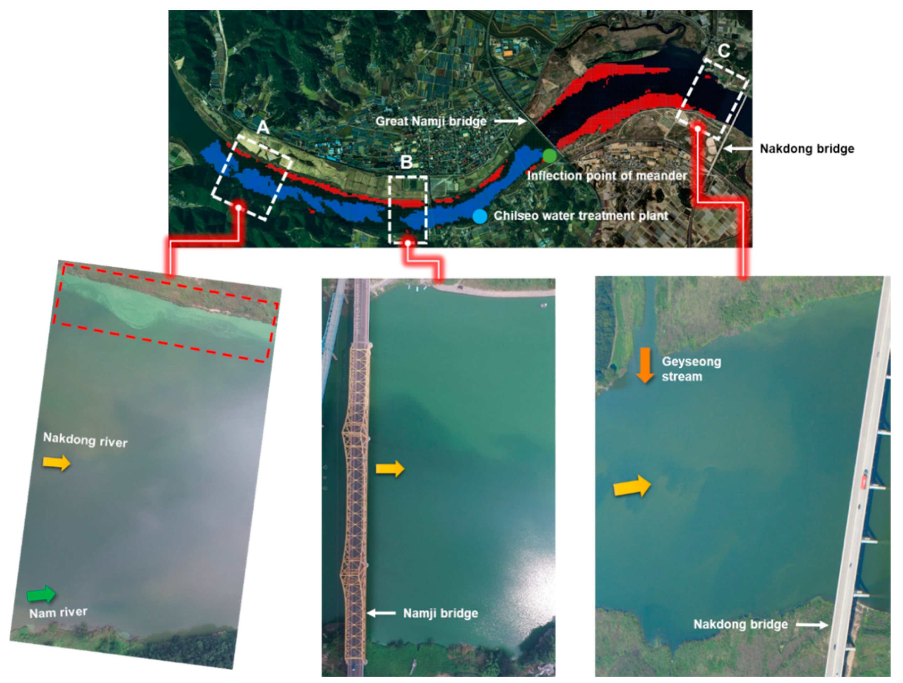
Figure 8 shows the UAV-monitoring results during a period of HAB occurrence based on a series of aerial photographs. We used a commercial drone (Fathom IV, DJI) to acquire the photographs over a period of approximately half of a day. The photographed results ensured that the UAV survey can provide useful information to spatially identify the current status of the algal blooms. This UAV-based survey entailed a low-altitude flight of approximately 100 m with continuous image recordings and spatial resolution at the sub-centimeter scale. To facilitate comparisons and interpretation of the results,
Figure 8 specifies the UAV monitoring areas by selecting three major local areas marked as A, B, and C above the HAB-prone regions based on the hot-spot analysis with Getis-Ord G*. These specified areas, i.e., A, B, and C, were mostly located at the upper, middle, and lower regions of the study area to individually represent the impacts of the confluence, meandering and adjacent water intake, and channel width expansion, respectively.
More specifically, area A is located at the immediate downstream section of the Nam River confluence. The UAV monitoring results showed that HABs appeared only along the left bank in area A, which was highly similar to the hot-spot analysis based on the Getis-Ord G*method. Such a textured pattern was simultaneously maintained downstream, whereas there was no visual indication of an algal bloom along the right side margin of the channel corridor. This result can be attributed to the intrusion of the Nam River. Nevertheless, we suggest that the presence of a very small red spot, as well as a black-colored area on the right margin from the Getis-Ord G* results, should be viewed with caution, although these spots are not as prominent they are from the K-means clustering method results. This indicates that the right side of area A may also be susceptible and of concern for algal blooms when they expand due to worsening conditions, despite the fact that no current and imminent algal blooms were identified on the day of UAV monitoring.
Area B is the downstream section of Namji Bridge, where the Chilseo water treatment plant has been in operation for the last several decades downstream of the photographed section. A visual comparison between the UAV-monitored photograph and hot-spot analysis revealed similar patterns where algae bloomed on the left side of the channel and became more developed toward the center of the channel, as compared with area A. Therefore, the coverage of the bloom expanded downstream on this side. In contrast, there was still an absence of algal blooms on the right side of the channel, which inherited the characteristics of the blooms identified in area A. These results also correspond to the results of the hot-spot analysis, thereby validating that the proposed method based on ADCP data can predict algal blooms as revealed by on our identification of the HAB-prone region in area B.
From this context, these findings can be extended to other practical applications as follows. In the absence of an HAB-prone area, as revealed by either the hot-spot analysis or UAV-monitoring at the beginning of the confluence, as observed in area A, this pattern persisted on the right side of the channel along the downstream region almost until Nakdong Bridge, arriving near the inflection point of the meandering direction, as illustrated in
Figure 8. This confirms that the contribution from the Nam River, in terms of suppressing HABs, persisted to the region where the tributary no longer has an influence, i.e., the completion of mixing. This is an important perspective when evaluating the safety of the drinking water intake located in the vicinity of area B (see
Figure 8), where harmful microcystins residing in the blue-green algae can significantly threaten public drinking water intake systems. Given that the mega-cities surrounding the intake, such as Daegu and Busan, heavily rely on this specific drinking water intake, significant concerns have subsequently emerged after the continual occurrences of annual algal blooms in this river corridor with the completion of the four major river projects in 2012 [
1,
2]. Therefore, whether this water intake is be directly affected by HABs and the type of influence that intrusion from Nam River has on these HABs at this point are critical issues. Based on observations of the location of Chilseo intake, adjacent to area B, we can observe that this location is out of the range of the HAB-prone area. The results from this study indicate that the algal bloom did not initiate in the area near the intake on the right side of the channel, rather it tended to initiate at the opposite side of the channel owing to the influence of Nam River. Collectively, the intake is able to maintain its quality due to Nam River, i.e., its quality is not maintained by Nakdong River with algal blooms; therefore, this station and its drinking water are safe until the outbreak of a significantly large algal bloom. The above results, therefore, also reveal the novelty of this study with the use of ADCPs, which can conveniently delineate whether certain critical areas, such as a water intake station, will be prone to HABs before the algae season. However, we note that once a very large algae outbreak (e.g., more than one million cells per liter) dominated all of the river channels, the intake was affected by harmful algae, as previously reported in the press.
Finally, area C is located in the downstream region of Namji Bridge (
Figure 8), which is characterized by an overall lower bathymetry, as compared with the upstream river corridor, a wide channel width, a slow flow velocity, a high water surface temperature, and a large backscatter. Thus, area C may be highly prone to algal blooms, whereas the area before Namji bridge is deeper and faster. However, due to the meandering feature, the right side of the channel in area C was characterized by a slower and shallow flow regime, as shown in
Figure 8, such that it may be prone to algal blooms. At this point, the positive influence from Nam River has disappeared before this area, which prevailed in areas A and B, enabling the dilution of the main channel river; however, a small tributary, i.e., Gyeseng stream, enters the main channel in area C from the left side of the channel near the apex of the meander (see
Figure 8). This stream can be another source of nutrients or clean water from a small rural watershed, as well as the ability to play a role, to a certain degree, in expanding the channel geometry. Notable generic features are that the HAB-prone area derived from the ADCP data revealed that both the right and left sides of the channel yield hot-spots with red-colored areas (see area C in
Figure 8), whereas the center region was undetermined and more susceptible than the cold spot. Although the reason for the lack of HABs in this region is not clear and a number of factors are open to debate, we can suggest several hypotheses. For instance, the intrusion from Geyseong stream on the left side apex of the channel results in the temporary disappearance of the algal bloom. Overall, the algae emerged and proliferated in area C as a consequence of the aforementioned conditions, which were similarly confirmed by the UAV-based photograph. In terms of a visual inspection of the aerial photograph, however, the textured features of the algal bloom were more complex than predicted and, strictly speaking, the area in the photograph appeared slightly different in detail from that obtained with the hot-spot analysis. In reality, the algal bloom had already, to a certain extent, expanded from both banks toward the center of the channel, despite the fact that the spatial concentration of algal blooms was characterized by a lower degree. Although not clearly identified, the intrusion from Geyseong stream appears to have disturbed the spatial pattern and added a certain degree of complexity.
3.5. Challenges and Lessons Learned
This study predicted HAB hotspots using the temperature, depth, flow velocity, and backscatter data measured using an ADCP. Considering that most current studies on fluvial monitoring for algal blooms are locally limited, not cost-effective, laborious, and had to rely on remote sensing data, this method is consistent with remote sensing results, despite possible applicability constraints that do not include water quality data. ADCP has emerged throughout the last several decades and hydrometric communities and agencies around the world have accumulated ADCP measurements intended for various riverine applications, such as developing stage-discharge rating curves in diverse stages and flow regimes. Based on the availability of large ADCP datasets, this study proposed a practical technique to evaluate HAB-prone regions with legacy ADCP data without further supplementary data collection, such as water quality. The comparative results with actual algal blooms revealed that the ADCP is feasible for the forecasting of HAB-prone regions with minimum preparedness and expense. In other words, we expect that this method will improve our capabilities of ultimately gaining a measure to forecast HAB-prone regions based solely on ground-based monitoring.
However, there are certain issues that occurred during the development and validation of this procedure. Therefore, we provide a brief overview of the main challenges and lessons posed by environmental restrictions, tools, and data.
First, the proposed idea and methods for deriving undesirable HAB-prone areas was scrutinized using a case study of in situ ADCP measurements. For this reason, the present analysis and conclusions herein are based on a limited dataset; thus, the findings and validations remain preliminary. From this perspective, our outcomes should be regarded as indicative rather than confirmative. Further studies are therefore required to more precisely validate the proposed method. In contrast, the validation of the derived HAB-prone regions was conducted at a specified moment associated with the actual presence of HABs. Considering that the degree of severity of HABs can be interpreted differently over time and the analysis results in the synthetic plots reported in this study provide a specific case in which ADCP measurements preceded three months of subsequent development, current outcomes cannot separately account for different phases of algal blooms. As a consequence, we recommend more thorough studies for other temporal situations associated with algal blooms. Based on this study, however, we can stress that it is important to delineate areas susceptible to the initiation and development of algal blooms, which, for example, can occur in areas with the presence of a dead zone along the channel perimeter.
Second, this method can improve the flexibility of forecasting HAB-prone regions, allowing preemptive responses such as aeriation and chemical controls to substantial algal blooms, which enables us to develop elaborate countermeasures to mitigate the further proliferation of HABs by identifying where to begin and the isolation of that area. Hence, we can benefit from simple ADCP measurements with no other additional measurements. In general, seeds of algae locally distributed in a randomly segmented form particularly begin to grow in certain locations with highly suited preferable conditions. Therefore, this initial moment, at which the algae have not significantly bloomed, is the period when various bloom management methods should be performed, such as biomanipulation, soil drop, and physical elimination, enabling us to counteract and deteriorate algal blooms before their full proliferation overwhelms management capacities. This means that the abundance of legacy ADCP measurements, which numerous hydrometric agencies have accumulated over previous decades, can offer an effective preemptive approach to prevent massive algal blooms.
Third, given the acceptable agreement between the forecasted HAB-prone regions based on the ADCP measurements and the regions of actual algal blooms, the ADCP-based approach possibly allows for the precise identification or characterization of algal bloom, as opposed to the paucity of comprehensive datasets, including water quality. HAB-prone regions may form due to multiple reasons. Current methods cannot discern the type of algae due to the fact that different types of algae can prefer similar hydro- and morpho-dynamic riverine conditions. The addition of a water quality dataset, therefore, can place better constraints on the prediction of HAB-prone regions. However, we note that, in general, water quality data are only available at a limited fixed point instead of a large spatial coverage, as is the case for ADCPs. In the absence of such spatially distributed water quality data, the central theme of this study is the ability to fully utilize the valid benefits of ADCPs. Despite a decrease in the degree of accuracy and identification capacity type, ADCPs remain highly practical for forecasting HAB-prone regions.
Fourth, the majority of existing solutions for understanding the life cycles of algal growth have relied on sophisticated physically-based numerical simulations and calibrated point-based sporadic observations of agal blooms. In parallel, rapid advances in remote sensing technologies have shown significant potential for solving various research issues related to algal blooms, allowing the coverage of a riverine space with unprecedented efficacy. In contrast, this method relies on conventional ground-based direct measurements and subsequent data-driven modeling, such that this approach can be limited with respect to the accommodation of a broad range of flow environments and applications. Therefore, we suggest that the proposed method should be incorporated into a hybrid form with numerical models and remote sensing techniques.
4. Conclusions
The novelty of this study is the utilization of ADCP data to conjunctively identify HAB-prone regions. The proposed method aimed to develop a practical and rapid countermeasure, enabling a preemptive response to massive algal blooms, through which we can identify HAB-prone regions based on estimations of where harmful algae initiate and develop significant prior to the algal bloom season. We anticipate that this method can be used to mitigate ongoing environmental threats posed by unprecedented HABs, as well as for understanding algal blooms in freshwater systems. Considering relatively few studies have documented the performance and accuracy of using ADCP data to derive HAB-prone areas, this study highlights the usability of conventional acoustic methods and datasets, which have, to date, been massively accumulated by hydrometric communities. With a strategic combination of various ADCP measurement data to forecast HAB-prone regions, on the other hand, the method can be extended to encompass other emerging measurement techniques subsequently corroborated with measurements of water quality, which can provide a full description of the algal bloom process and their evolution. UAV surveys can offer useful complementary information on the monitoring of algal blooms, combined with emerging trends that will shape the best management practices to control HABs. We discussed the benefits and disadvantages of the proposed method, concluding that there is a need for further investigations to validate the feasibility of the proposed method by determining and optimizing all the available parameters. Tentatively, the Getis-Ord G* method yielded a better performance through comparative visual inspection, as compared with the photographs generated by UAV-based algal monitoring. Collectively, this method shows potential for forecasting HAB-prone regions, allowing preemptive responses before massive algal blooms, enabling the development of elaborate countermeasures to mitigate the further proliferation of HABs by identifying areas for isolation. We anticipate that this method can be used to mitigate ongoing environmental threats posed by unprecedented harmful algal blooms, as well as for understanding the formation and evolution of algal blooms in freshwater systems. These tools were assembled with the intent to aid and facilitate the forecasting HABs, followed by the application of measures to mitigate HABs and assess their degree. This approach can be readily applied by engineering or field operators.


