Geophysical Assessment of Seawater Intrusion into Coastal Aquifers of Bela Plain, Pakistan

Abstract

Seawater intrusion is a major challenge in many coastal areas all around the world, mainly caused by over-exploitation of freshwater resources, climate change, and sea-level rise. Consequently, seawater intrusion reaches several kilometers inland, thus making the freshwater resources polluted and unsuitable for human use. Conventionally, the fresh-saline water interface is delineated by the number of laboratory tests obtained from boreholes. However, such tests suffer from efficiency in terms of data coverage, time, and cost. Hence, this work introduces Dar-Zarrouk (D-Z) parameters, namely transverse resistance (T_r), longitudinal conductance (S_c), and longitudinal resistivity (ρ_L) computed from non-invasive vertical electrical sounding (VES). Two-dimensional (2D) imaging of D-Z parameters provides a clear distinction of fresh-saline aquifers. Such techniques remove ambiguities in the resistivity interpretation caused by overlapping of fresh and saline aquifers during the process of suppression and equivalence. This study was carried out by 45 VES along five profiles in the coastal area of Bela Plain, Pakistan. D-Z parameters delineate fresh, brackish, and saline aquifers with a wide range of values such as freshwater with T_r > 2000 Ωm², S_c < 3 mho, and ρ_L > 20 Ωm; saline water with T_r < 1000 Ωm², S_c > 25 mho, and ρ_L < 5 Ωm; and brackish water with T_r between 1000–2000 Ωm², S_c from 3 to 25 mho, and ρ_L between 5–20 Ωm. The D-Z results were validated by the physicochemical analysis using 13 water samples and local hydrogeological setting. The obtained results propose that D-Z parameters can be used as a powerful tool to demarcate the fresh-saline aquifer interface with more confidence than other traditional techniques. This geophysical approach can reduce the expensive number of borehole tests, and hence contributes to the future planning and development of freshwater resources in the coastal areas.

1. Introduction

In Pakistan, groundwater is an essential resource for sustaining the population and economy [1]. Recently, groundwater utilization in the coastal areas has increased to meet water demand for industrial, agricultural, domestic, and tourist uses [2]. Consequently, improper management, excessive development, and over-exploitation of freshwater have deteriorated both the quantity and quality of groundwater reserves [3]. The main concern is seawater intrusion, which has resulted in groundwater contamination and well reduction [4,5]. Seawater intrusion is a natural occurrence caused by the density difference between seawater and freshwater. Seawater intrusion occurs when, due to the over-extraction of groundwater resources, outflow exceeds the aquifer recharge which is dynamically connected to the sea [6,7]. Generally, problems arise, when the seawater enters the aquifer system due to excessive pumping beyond the natural recharge rate, or when the potentiometric surface lowered by the extreme pumping at local individual wells causes the upcoming of the natural boundary between saline water and freshwater [8,9]. In addition, coastal aquifers are sensitive to the sea level rise due to global warming, and the melting snowcaps add to the level of seawater encroachment and ease the accessibility of freshwater reserves [10]. Therefore, demarcation of the fresh-saline groundwater boundary is very important for extraction and management of freshwater reserves in the coastal areas.

Delineation of the saltwater intrusion has become a global issue within the last century. In the last two decades, many studies around the world were conducted to assess the fresh/saline aquifers [1,2,10,11,12,13,14]. Classically, seawater intrusion is monitored using the physicochemical analysis of groundwater samples and piezometry through the measurements of water-level fluctuations [15,16]. For successful monitoring of saltwater encroachment, observation wells are required to be dispersed over the entire investigated area. However, the economic reason mainly causes the sparse density of test wells, and thus the distributed wells do not characterize the total area sufficiently [17]. With the intent to ease the lack of information and improve the monitoring of the aquifer system, an efficient technique is necessary. The surface geophysical methods such as vertical electrical sounding (VES) are known as one of the most proficient techniques to assess groundwater resources quantitatively and qualitatively [18,19,20,21]. Electrical resistivity is extensively used to delineate seawater intrusion into coastal aquifers. A clear difference in resistivity values of freshwater and saltwater is useful to assess the fresh-saline water interface in the coastal areas [22,23]. Low resistivity values show saltwater, whereas high values suggest freshwater. Subsurface resistivity depends on many factors such as water content, saturation degree, porosity, rock type, soil type, salinity, and mineralization of groundwater, etc. [12]. Conversely, some geophysical similarities cause uncertainty in the resolution. Sometimes, the interpretation shows an intermixing of resistivity values for fresh and saline groundwater [24]. Dar-Zarrouk (D-Z) parameters can remove the overlapping of fresh/saline aquifers, and provide a more certain, practical, and reliable solution to the interpretation [11,25]. Applications of the D-Z parameters, namely transverse resistance, longitudinal conductance, and longitudinal resistivity computed from VES measurements mark a clear boundary between saline and fresh groundwater. Many studies have used D-Z parameters for delineation of the fresh-saline aquifer interface [1,11,12,17,25]. However, these studies provide only a 1D (one-dimensional) delineation of fresh-saline aquifer. Mostly, ERT is used to delineate the 2D demarcation of fresh-saline groundwater, however, ERT cannot cover a large area. In order to get a clear insight into the fresh-saline aquifer, the 2D delineation of the aquifer system is essential. This work provides a new innovative approach for the 2D demarcation of fresh-saline aquifer using the D-Z parameters. Based on local geological settings and groundwater conditions, D-Z parameters were acquired for each distinct layer of fresh or saline water with various arrangements of resistivity and thickness. These parameters delineated saline and fresh aquifers with a wide range of specific values depending on local hydrogeological conditions and wells information. Freshwater was delineated by high values of transverse resistance and longitudinal resistivity but low values of longitudinal conductance, whereas saltwater was assessed with high values of longitudinal conductance but low values of the two other parameters.

During the last two decades, the coastal aquifers of Bela Plain have become polluted due to the over-extraction of groundwater resources mainly for agriculture demand. Groundwater, with seawater intrusion of more than 50 km from the Sonmiani Bay of Arabian Sea towards the inlands of the study area, has become unsuitable for drinking and agriculture purposes. The number of boreholes near the coast is discarded due to seawater intrusion. The main aim of the present investigation is to emphasize the application of D-Z parameters derived from VES data for 2D mapping of seawater intrusion into coastal areas of Bela Plain, Pakistan, and to display how this non-invasive geophysical technique can be used to reduce the number of expensive well samples of hydrogeochemical information. In addition, the monitoring boreholes data of physicochemical parameters were integrated with a geophysical interpretation to improve and validate the results of the D-Z parameters for the assessment of saline and fresh aquifers.

2. Study Area and Hydrology

Bela Plain is located in Lasbela District covering an area of 3100 km². The study area is situated south of the Baluchistan Province between latitiude 25–26.55° N and longitude 66–67° E. Bela Plain is surrounded by hills of sedimentary rocks from three sides in the east, west, and north and Sonmiani Bay (Arabian Sea) in the south (Figure 1). The study area is located in the arid region having an average annual precipitation of 80–130 mm, high evaporation, and low recharge to groundwater. Agriculture is the main source of earning for people in the study area, which mainly relies on tubewells, streamflow, and rainfall. The investigated area has intermittent streams mostly, and the only perennial one is the Porali River in the southeast. The alluvial cover of unconsolidated deposits was formed during the quaternary age, and the errosion processes shaped the topographic relief of the study area.

The stream runoff and rainfall are the main sources of water in foothills and piedmont areas of Bela Plain. In northern areas, groundwater is mainly recharged by streamflows of Porali River through permeable beds. Whereas, rainafll is mainly the source of groundwater recharge for the rest of the areas in Bela Plain. In northern Mor and Par Ranges, Porali River at the Sinchi Bent guaging station, is the major source of water with an irrigation land of 4039 km². The surface water hydrology, WASID (water and soil investigation division) is responsible for meausring the discharge rate of rivers and streams in the study area [26]. The mean annual flow is 120 million m³, which is mostly used in agriculture [27]. About 14–18 km downstream from the Sinchi Bent guaging station, Kud River joins the Porali River. At Mai Gondrani, the mean annual flow is 102 million m³ [27]. Windar Nai with a drainage area of 1733 km² is a non-perennial stream, which direcly flows into the Arabian Sea in the south. Khantra Nai is another main non-perennial stream in the study area.

Gravel, sand, clay, and silt are the main lithologies in the investigated area as revealed by the drilling tests. However, gravel forms the most extensive and permeable aquifer, which lies in the unconsolidated deposits under the alluvial fans and piedmonts places. Generally, the study area has the unconfined aquifer system. However, the semi-permeable beds of silt and clay are dominant in the south and southwest parts where they make the confined aquifer sytem with saltwater. The water table varies between 0–15 m in the investigated area. The shape of the water table depth is of concave type in the southwest and middle of the investigated area along Porali River and Khantra Nai. The groundwater recharge rate is mainly controlled by the seasonal conditions of discharge from the surfacewater into the groundwater. The general flow direction of surface water in Bela Plain is from the northeast to the southwest towards the Arabian Sea. This investigation was conducted by the Water And Power Development Authority, Pakistan (WAPDA) under a project in order to assess seawater intrusion into the coastal area of Bela Plain for the development and management of freshwater resources. All the 45 VES were performed in the same time period/season (April/May, 2017) as the groundwater samples were collected from the 13 wells. The location of VES and wells inluding the hydrogeological setting of the investigated area is given in Figure 1a. Figure 1b shows a schematic diagram of seawater intrusion into the coatsal aquifer.

3. Materials and Methods

3.1. VES Survey

Seawater intrusion into coastal aquifers is delineated by many techniques. It is never easy to directly interpret the measurements of apparent electrical conductivity quantitatively, since it depends on several properties, such as clay containing high concentrations of cations and dissolved electrolytes, temperature, porosity, etc. [28]. In addition, a high electrical conductivity shows saltwater, whereas its low values suggest freshwater [11]. This difference between the electrical conductivity of freshwater and saltwater is highly significant, and therefore, the VES method is more suitable to assess the fresh-saline groundwater interface in the coastal regions [29]. Geophysical methods such as vertical electrical sounding (VES) are widely used in environmental and hydrogeological studies given their ability to incorporate with other methods, such as hydrochemical and geological methods, through a comprehensive interpretation. A useful correlation is found between hydraulic and electrical properties of the saturated geological formations, which make the geoelectrical methods even more effective in such studies [30,31,32,33]. An integrated approach of the VES and geochemical method in combination with hydrogeological data has been used to evaluate the characteristics of groundwater and delineate the expansion of seawater intrusion into the coastal aquifer.

In this research, a VES survey was performed to compute the subsurface resistivity. Electrical resistivity depends on the characteristics of subsurface materials, such as rock texture, nature of mineralization, and electrical conductivity [34]. It varies from formation to formation. Coarse grains show high values of resistivity, whereas an increase in the clay content or salinity gives low values. In the VES survey, an electric current is injected into the subsurface through two electrodes known as current electrodes, and two other electrodes namely potential electrodes are used to measure the electrical potential. The measured voltage is converted into the resistance value using the resistivity meter. The anomalies are observed by plotting the resistance values on a log-log paper in the field. With each resistivity measurement, spacing between the current electrodes is increased to acquire the large depth of investigation. The signal to noise ratio is enhanced by increasing spacing between the inner potential electrodes. In this survey, 45 VES measurements (Figure 1a) were acquired by a resistivity meter (Syscal R1 Plusmodel, Iris) using the Schlumberger array. The VES data points were divided into five profiles, i.e., A, B, C, D, and E as shown in Figure 1a. The spacing of current electrodes (AB) and potential electrodes (MN) was adjusted at all depths according to a relationship, i.e., 2(AB/2) > 5 MN [35]. The minimum and maximum half-current electrodes spacing (AB/2) was used as 1 and 200 m, respectively, whereas the potential electrodes spacing (MN) varied between 0.25–20 m. The resistivity measured directly from the VES data is apparent resistivity. This resistivity needs to be inverted, as it does not represent the true values of subsurface layers [36]. The apparent resistivity data were inverted by the IPI2WIN software version 3.1.2c, developed by Moscow State University [37]. The software program compared the theoretical curve with the inverted (true) resistivity and the calibrated field curve (Figure 2a). The shape of the modeled VES curves shows variations in different layers with different resistivities [35]. The VES models divide the subsurface formation into distinct layers with a specific value of thickness and resistivity. The correct interpretation of VES models is performed using the local information acquired from boreholes data and hydrogeological setting.

3.2. Dar-Zarrouk Parameters

Occasionally, the VES interpretation causes ambiguity in the resolution and resistivity values, which shows the overlapping of demarcation of saline and fresh groundwater [24]. D-Z parameters remove any such uncertainty in the resistivity interpretation, and provides a clear interface between the freshwater and saltwater. They present a more practical, definite, and reliable solution to the interpretation [11,25]. D-Z parameters mark a clear interface between saline and fresh groundwater with a wide range of their values without overlapping of values or aquifers. D-Z parameters, namely transverse resistance (T_r), longitudinal resistivity (ρ_L), and longitudinal conductance (S_c) were first introduced by Mailet in 1947. These parameters offer sufficient resolutions to subsurface resistivity for the delineation of seawater intrusion [11]. They efficiently mark a distinct boundary between saline and fresh groundwater with a specific range of their values [12]. These parameters are estimated through different arrangements of thickness and resistivity acquired from the VES models (Figure 2b), and thus they give a better understanding of the subsurface discrete layers for the evaluation of a boundary between saline and fresh groundwater [11,38,39]. Any geoelectrical layer in a VES model is defined by two fundamental properties, namely resistivity (ρ) and thickness (h) [40]. Various arrangements of resistivity (ρ) and thickness (h) for each lithologic unit of VES model describe the D-Z parameters [11,41]. Transverse resistance was estimated by the following arrangement of h and ρ [11,41]:

$$\mathrm{Tr} =\left(h\right)\left(\rho \right)$$

(1)

where h and ρ are the aquifer thickness and resistivity of each layer in the VES model. T_r is the transverse resistance measured in units of Ωm². Longitudinal conductance was calculated by the following formula [11,41]:

$${\mathrm{S}}_{\mathrm{c}} =(\frac{h}{\rho } )$$

(2)

where S_c is the longitudinal conductance of each saturated layer, and it is measured in Siemens (mho). The longitudinal resistivity is acquired using the following equation [11,41]:

$${\rho }_{\mathrm{L}}=(\frac{h}{{\mathrm{S}}_{\mathrm{c}}})$$

(3)

where ρ_L is the longitudinal resistivity of each layer, and is estimated in Ωm. Equations (1)–(3) were used to estimate the D-Z parameters of each distinct layer of the VES model (Figure 2b). D-Z parameters were estimated for all 45 VES models to get the 2D mapping of discrete saline and fresh groundwater in Bela Plain. Specific values ranges of T_r, S_c, and ρ_L for saline, brackish, and fresh aquifers were obtained based on the hydrogeological setting and wells information of the investigated site. To obtain specific values ranges of the D-Z parameters, the lithological logs data of the 13 wells were integrated with the D-Z parameters of the selected 13 VES nearby the wells. An example of such integration between the selected VES 9 and the lithological well log 3 is shown in Figure 2a. However, these values ranges of D-Z parameters are not unique and may vary from area to area based on the local hydrogeological setting.

3.3. Geochemical Method

The physicochemical analysis was conducted for 13 groundwater samples obtained from the pumping wells with an average depth range of 60–110 m. The laboratory analysis of groundwater samples was conducted using the ion chromatography technique by the Pakistan Council of Research in Water Resource (PCRWR). The physicochemical study was performed by the recommended limits of the World Health Organization [43] for main anions such as chloride (Cl⁻), sulphates (SO₄²⁻), nitrate (NO₃⁻), and bicarbonates (HCO₃⁻), as well as main cations including magnesium (Mg²⁺), sodium (Na⁺), potassium (K⁺), calcium (Ca²⁺), and other geochemical parameters such as electrical conductivity (EC), pH, and total dissolved solids (TDS) [44]. The standard procedures method was used to determine the concentrations of calcium, bicarbonate, sodium, sulphate, potassium, chloride, and magnesium [44]. Bicarbonates and chlorides ions were obtained by the volumetric method. The UV–visible spectrophotometer was applied for the analysis of sulphates. The atomic absorption spectrometry was performed to analyze the main cations. The concentration of cations and anions was measured in milligrams per liter (mg/L). The concentration of the electrical conductivity in microsiemens per centimeter (μS/cm) was determined at 25 °C. The consistency of the groundwater quality parameters was confirmed using the ionic balance of water, and the acceptable reliability was found between +5% and −5%.

4. Results

4.1. Interpretation of Resistivity Data

Resistivity measured in the field is not a true representative of subsurface geologic units, and therefore, apparent resistivity is inverted to true resistivity through an inversion procedure of the software [1]. Resistivity varies even with a minor change in lithology. The resistivity of sand is lower than the resistivity of gravel, similarly, the resistivity of silt/clay is lower than that of sand. Moreover, freshwater shows a high resistivity, while saline water indicates a low resistivity. Mostly, gravel/sand reveal freshwater, whereas clay delineates saltwater [12]. However, with a homogeneous and anisotropic subsurface, uncertainties can be expected in VES methods for the characterization of subsurface lithologies [36]. Therefore, the VES models and local hydrogeological information obtained from wells are correlated to constrain the subsurface into discrete lithologic layers. In this study, the non-predictive bias evaluation of the subsurface was obtained by correlating 45 VES models with lithological logs of 13 boreholes (

Table 1. Overlapping in resistivity values and lithologies obtained after calibration between the local boreholes information and subsurface resistivity in Bela Plain.

Subsurface Resistivity (Ωm)	Lithology Type	Overlapping
		Resistivity	Lithology	Aquifer
>35 (above water table)	Topsoil cover (dry strata)	-	-	-
<7 (below water table)	Clay (saline water)	4–7	Clay and Clay-sand	Saline-brackish
4–24 (below water table)	Clay-sand (brackish water)
		18–24	Clay-sand and sand	Brackish-fresh
18–42 (below water table)	Sand (freshwater)
		34–42	Sand and gravel-sand	-
34–60 (below water table)	Gravel-sand (freshwater)
		50–60	Gravel-sand and gravel	-
>50 (below water table)	Gravel (freshwater)

). A comparison between the interpreted VES 9 and lithological well log 3 is shown in Figure 2a. Similarly, the calibration (comparison) between the 45 VES models and 13 lithological well logs was performed to obtain a resistivity values range for each layer containing fresh-saline or brackish aquifer with specific lithology. This calibration delineated the subsurface into several lithological units, such as dry strata/topsoil cover (above water table) having resistivity >35 Ωm, clay (below water table) with saline water having resistivity <7 Ωm, clay-sand (below water table) with brackish water and resistivity between 4–24 Ωm, sand (below water table) having a freshwater and resistivity range of 18–42 Ωm, gravel-sand (below water table) with freshwater and resistivity from 34 to 60 Ωm, and gravel (below water table) having freshwater and resistivity >50 Ωm (Table 1).

The calibration shows that the interpreted layers have very narrow resistivity ranges with an overlapping nature. The clay of saline water having resistivity <7 Ωm intermixes with the clay-sand of brackish water with resistivity between 4–24, and thus causes an overlapping of saline-brackish aquifer with resistivity between 4–7 Ωm. Similarly, the clay-sand of brackish water having a resistivity range of 4–24 Ωm interferes with the sand of freshwater with resistivity from 18 to 42 Ωm, and hence creates an overlapping of brackish-fresh aquifer with a resistivity range of 18–24 Ωm. In addition, Table 1 shows the intermixing of sand with gravel-sand for resistivity overlapping of 34–42 Ωm, and gravel with gravel-sand for resistivity overlapping of 50–60 Ωm. Therefore, such overlapping causes an ambiguity in resolution for the separation between saline and fresh groundwater. This implies that the VES technique cannot interpret the subsurface with a high resolution, especially when the lithological units have some similarities, such as clay-sand and clay or sand and clay-sand. However, D-Z parameters estimated from the VES models can remove any such ambiguity, and thus provide a more confident resolution to the interpretation of fresh-saline aquifers. These parameters have a wide range of values to mark a clear interface between freshwater and saline water.

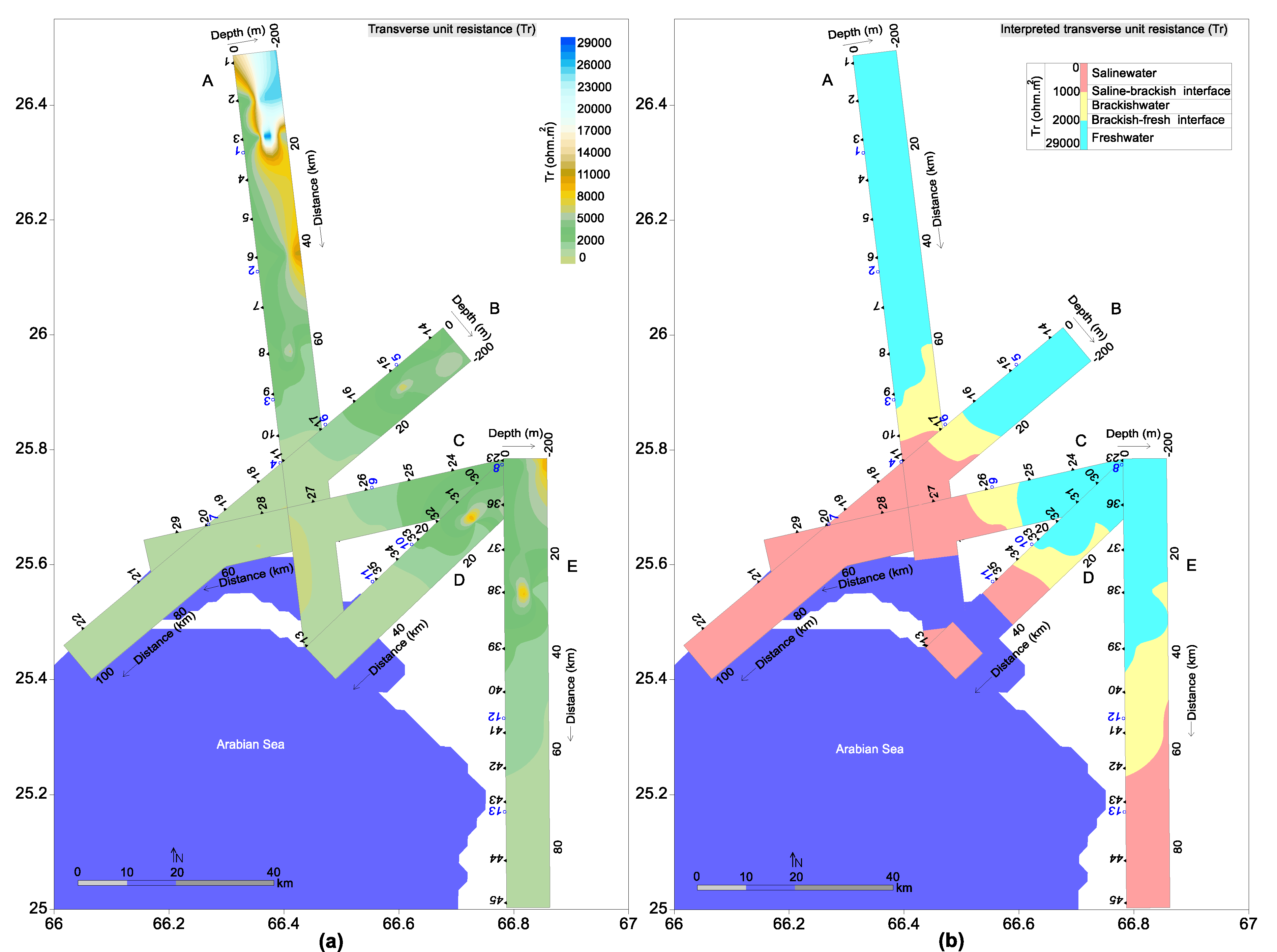
4.2. Transverse Resistance

An important parameter of the D-Z parameters, namely transverse unit resistance (T_r), was estimated for each layer of the 45 VES models along profiles A-E through the arrangement (Equation (1)) of aquifer thickness and resistivity of the layer. Transverse unit resistance was used to demarcate fresh, brackish, and saline water with a wide range of T_r values based on the wells information and hydrogeological setting of the investigated area. High values of T_r suggest that freshwater has sand or gravel as the main lithology, while its low values indicate saline water has clay as the main lithology. In this study, transverse unit resistance delineated saline water with T_r < 1000 Ωm² containing clay, brackish water with T_r between 1000–2000 Ωm² having clay-sand, and freshwater with T_r > 2000 Ωm² having sand, gravel-sand, and gravel (

Table 2. Study of Dar-Zarrouk (D-Z) parameters for the demarcation of saline, brackish, and fresh aquifers in Bela Plain.

D-Z Parameters	Range	Type of Aquifer	Overlapping
Transverse unit resistance (Tr)	>2000 Ωm2	Fresh	None
	1000–2000 Ωm2	Brackish
			None
	<1000 Ωm2	Saline
Longitudinal unit conductance (SC)	<3 mho	Fresh	None
	3–24 mho	Brackish
			None
	>24 mho	Saline
Longitudinal resistivity (ρL)	>20 Ωm	Fresh	None
	5–20 Ωm	Brackish
			None
	<5 Ωm	Saline

). The values range of T_r for fresh, brackish, and saline water shows no intermixing, which suggests that the aquifers delineated by T_r have no intermixing of saline-brackish or brackish-fresh aquifers.

The distribution of transverse unit resistance values over 45 VES in Figure 3a suggests that T_r increases from the sea (in the south) towards the inland (in the north). Based on the interpretation of T_r, Figure 3b provides the demarcation of saline, brackish, and fresh aquifers at different depths (50, 100, 150, and 200 m). At a 50 m depth, T_r varies between 50–4100 Ωm² with a T_r range of 50–574 Ωm² for saline water, 1280–1705 Ωm² for brackish water, and 2520–4100 Ωm² for freshwater. At a 100 m depth, the T_r values range is 10.9–36,400 Ωm² with T_r between 10.9–574 Ωm² for saline aquifer, 1280–1705 Ωm² for brackish aquifer, and 3000–36,400 Ωm² for fresh aquifer. At 150 and 200 m depths, T_r changes from 10.9 to 36,400 Ωm² having T_r of 10.9–92.8 Ωm² for saline aquifer, 1280–1705 Ωm² for brackish aquifer, and 2730–36,400 Ωm² for fresh aquifer. Generally, T_r (from 2520 to 36,400 Ωm²) for freshwater increases with depth, whereas T_r (from 574 to 10.9 Ωm²) for saltwater decreases with depth, which suggests seawater intrusion with an increasing depth (Figure 3b).

The 2D transverse unit resistance was obtained and interpreted for saline, brackish, and fresh groundwater along five profiles (A–E) (Figure 4a,b). Transverse unit resistance values vary along profile A to E with T_r between 11.3–28080, 8.8–6750, 11.5–9951, 11.3–9951, and 10.5–9951 Ωm², respectively (Figure 4a). Along profile A, the saline aquifer was delineated with T_r between 11.3–384 Ωm² for VES 11–13, brackish aquifer was revealed by T_r from 1386 to 1650 Ωm² for VES 8–10, and fresh aquifer was interpreted with a T_r range of 2700–28,080 Ωm² for VES 1–9 (Figure 4b). Seawater intrusion for profile A was observed about 45 km towards the inland along VES 8–13. Along profile B, freshwater was revealed by a T_r range of 2788–6750 Ωm² for VES 14–16, brackish water was interpreted with T_r of 1376 Ωm² for VES 16 and 17, and saline water was assessed with T_r between 8.8–384 Ωm² for VES 11 and 17–22 (Figure 4b). Seawater intrusion of about 75 km was found along this profile for VES 11 and 16–22. Along profile C, saline water was evaluated with T_r between 11.5–180 Ωm² for VES 20 and 26–29, brackish water was interpreted by T_r of 1440 Ωm² for VES 26, and freshwater was delineated with T_r between 3330–9951 Ωm² for VES 23–25 (Figure 4b). Seawater intrusion of 50 km was delineated along profile C with VES 20 and 26–29. Along profile D, freshwater was revealed by a T_r range of 2275–9951 Ωm² for VES 23 and 30–33, brackish water was interpreted with T_r between 1512–1705 Ωm² for VES 31–34, and saline water was delineated with T_r between 11.3–390 Ωm² for VES 13, 34, and 35 (Figure 4b). This profile reveals seawater intrusion of about 27 km along VES 13 and 31–35. Along profile E, saline aquifer was revealed by T_r between 10.5–560 Ωm² for VES 40–45, brackish aquifer was interpreted with T_r 1650–1700 Ωm² for VES 38–42, and fresh aquifer was delineated with T_r 2520–9951 Ωm² for VES 23 and 36–39 (Figure 4b). Seawater intrusion of about 65 km was revealed along profile E with VES 38–45. Figure 5a shows the integrated 2D maps of transverse unit resistance, and Figure 5b provides the demarcation of saline, brackish, and fresh groundwater for the integrated 2D T_r maps. Generally, seawater intrusion of about 27–75 km is delineated from the Arabian Sea in the southwest towards the inland of Bela Plain in the northeast (Figure 5b).

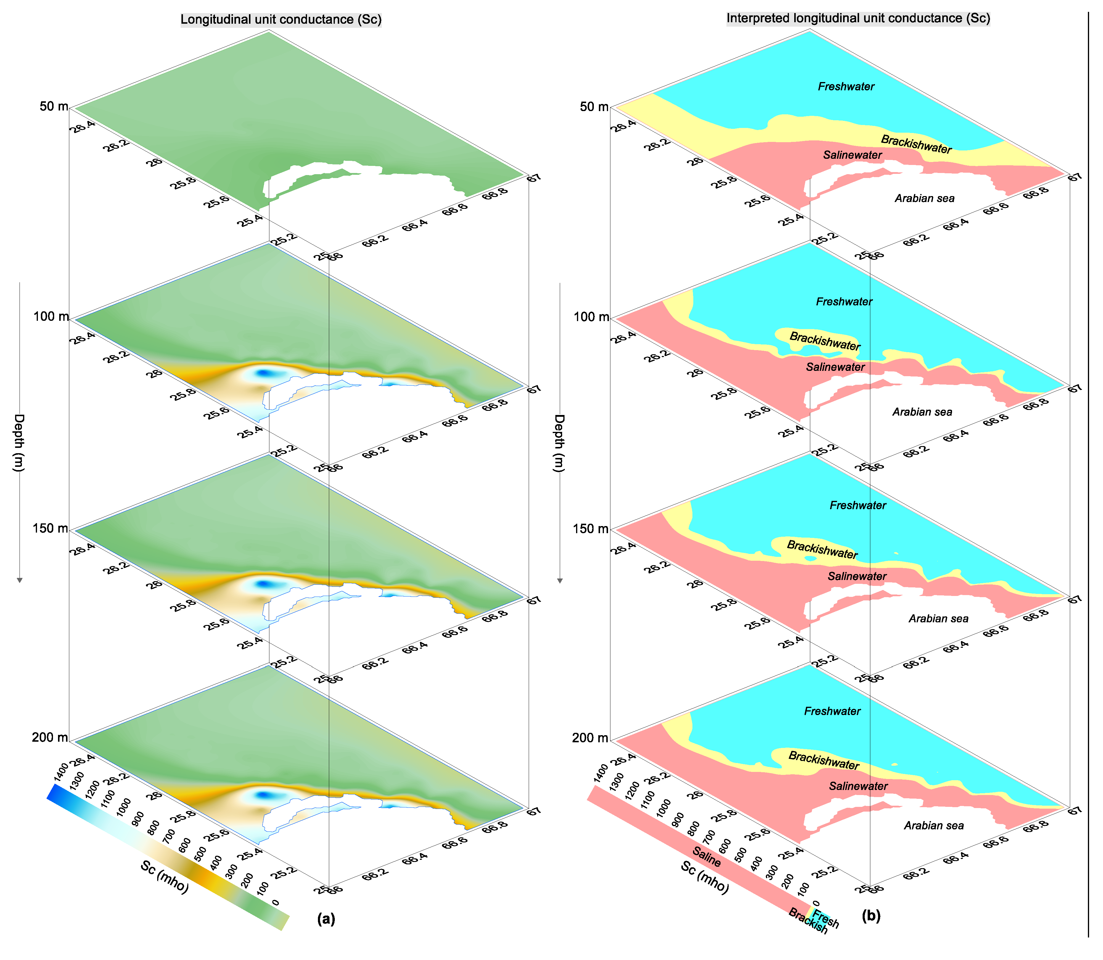
4.3. Longitudinal Conductance

Longitudinal unit conductance (S_c) was estimated using a combination (Equation (2)) of aquifer thickness and resistivity obtained from 45 VES models along profiles A-E. Based on the wells information and hydrogeological setting of the study area, a specific values range of longitudinal unit conductance was obtained to delineate fresh, brackish, and saline aquifers with a clear interface. Low values of S_c reveal freshwater with gravel-sand, whereas high values delineate saline water mainly with clay. Saline aquifer was delineated with S_c > 24 mho having clay, fresh aquifer was demarcated by S_c < 3 mho with sand, gravel-sand, and gravel, and brackish aquifer was interpreted with S_c between 3–24 mho containing clay-sand (Table 2). Figure 6a shows mapping of the longitudinal unit conductance, whereas the demarcation of saline, brackish, and fresh groundwater at different depths (i.e., 50, 100, 150, and 200 m) is given in Figure 6b. At a 50 m depth, longitudinal unit conductance varies from 0.7 to 80 mho with S_c between 34.1–80 mho delineating saline aquifer, 14–21.5 mho demarcating brackish aquifer, and 0.7–2.4 mho revealing fresh aquifer. At a 100 m depth, S_c ranges from 0.15 to 1460 mho having S_c between 34.1–1460 mho for saline aquifer, 13.6–21.5 mho for brackish aquifer, and 0.15–2.4 mho for fresh aquifer. At a 150 m depth, S_c varies between 0.23–1460 mho with a S_c range of 80–1460 mho revealing saline aquifer, 4.1–21.5 mho delineating brackish aquifer, and 0.23–2.2 mho interpreting fresh aquifer. At a 200 m depth, S_c ranges from 0.07 to 1460 mho with S_c between 42–1460 mho for saline aquifer, 4.1–20 mho for brackish aquifer, and 0.07–2.2 mho for fresh aquifer. Longitudinal unit conductance values for saline water increase with depth from 34.1 to 1460 mho and decrease for freshwater with depth from 2.4 to 0.07 mho, and thus suggest an increase in seawater intrusion with depth (Figure 6b).

The 2D mapping of longitudinal unit conductance and the interpreted zones of fresh, brackish, and saline water along profiles A–E are shown in Figure 7a,b. The longitudinal unit conductance varies along profile A to E with S_c between 0.15–1130, 0.07–1090, 0.1–1150, 0.1–1130, and 0.1–128 mho, respectively (Figure 7a). The fresh-saline aquifers interpreted by S_c are given in Figure 7b. Along profile A, saline aquifer was demarcated by S_c from 37.5 to 1130 mho for VES 10–13, brackish aquifer was delineated with S_c between 4.28–16.5 mho for VES 4–11, and fresh aquifer was revealed with S_c ranging from 0.15 to 2.28 mho for VES 1–10. Seawater intrusion of about 80 km was delineated along profile A for VES 4–13. Along profile B, fresh aquifer was assessed by S_c ranging from 0.07 to 2.4 mho for VES 14–16, brackish aquifer was revealed with S_c of 21.5 mho for VES 15–17, and saline aquifer was demarcated with S_c between 37.5–1090 mho for VES 11 and 16–22. This profile delineated seawater intrusion of about 90 km along VES 11 and 15–22. Along profile C, saline water was interpreted by S_c from 45 to 1150 mho for VES 20 and 24-29, brackish water was delineated with S_c of 17.8 mho for VES 24–26, and freshwater was evaluated with S_c between 0.1–2.43 mho for VES 23–25. Seawater intrusion of 60 km was revealed along profile C with VES 20 and 24–29. Along profile D, freshwater was identified with S_c between 0.9–2.4 mho for VES 23 and 30–34, brackish water was interpreted by a S_c range of 4.67–14.1 mho for VES 30–34, and saline water was demarcated with S_c from 35.76 to 1130 mho for VES 13, 34, and 35. This profile reveals seawater intrusion of about 35 km along VES 13 and 30–35. Along profile E, saline aquifer was delineated with a S_c range of 35–128 mho for VES 40–45, brackish aquifer was interpreted by S_c from 5 to 17 mho for VES 37–42, and fresh aquifer was assessed by S_c ranging from 0.1 to 2.43 mho for VES 23 and 36–39. Seawater intrusion of about 75 km was delineated along this profile with VES 37–45. Figure 8a provides the integration of 2D S_c maps. The fresh, brackish, and saline aquifers delineated by the integrated 2D S_c maps over the entire study area are given in Figure 8b. The integration of 2D S_c maps delineates seawater intrusion of about 35–90 km from the seaside in the southwest towards the investigated area in the northeast (Figure 8b).

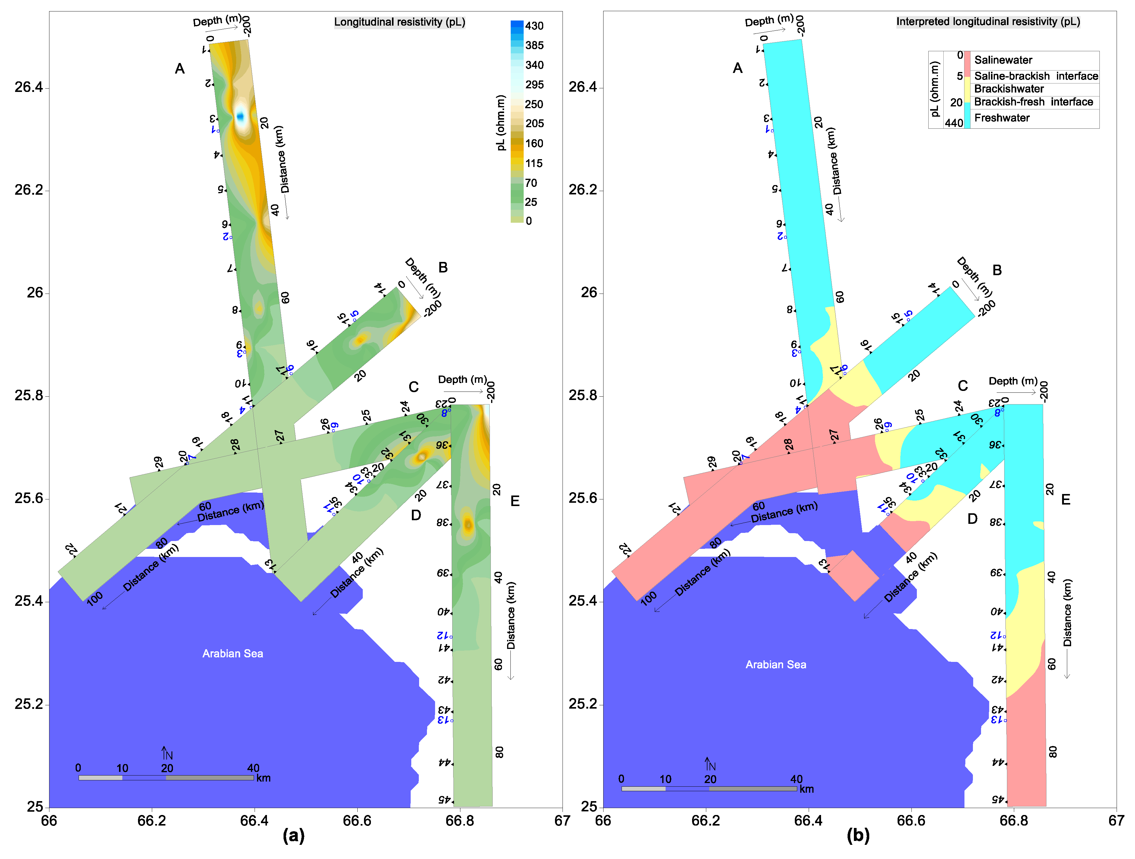
4.4. Longitudinal Resistivity

Longitudinal resistivity (ρ_L) was estimated for 45 VES models along profile A–E from a relation (Equation (3)) obtained by the arrangement of aquifer thickness and longitudinal conductance. Longitudinal resistivity revealed saline, brackish, and fresh aquifers with a wide range of values based on local hydrogeological setting and wells information. Generally, a high ρ_L suggests freshwater mainly with gravel-sand, while a low ρ_L reveals saline water with clay as the dominant lithology. In this investigation, longitudinal resistivity delineated the saline aquifer with ρ_L < 5 Ωm having clay, the brackish aquifer with ρ_L from 5 to 20 Ωm containing clay-sand, and freshwater with ρ_L > 20 Ωm having sand, gravel-sand, and gravel (Table 2). Mapping of the longitudinal resistivity over 45 VES is given in Figure 9a. The demarcation of fresh, brackish, and saline aquifers at different depths (50, 100, 150, and 200 m) is shown in Figure 9b. At a 50 m depth, ρ_L values vary between 1–60 Ωm with ρ_L range of 1–4.1 Ωm for saline aquifer, 8–11 Ωm for brackish aquifer, and 34–60 Ωm for fresh aquifer. At a 100 m depth, ρ_L ranges between 0.1–432 Ωm with ρ_L between 0.1–4.1 Ωm for saline aquifer, 8–11 Ωm for brackish aquifer, and 37–4320 Ωm for fresh aquifer. At 150 and 200 m depths, ρ_L varies between 0.1–350 Ωm having ρ_L of 0.1–0.9 Ωm for saline aquifer, 8–18 Ωm for brackish aquifer, and 35–350 Ωm for fresh aquifer. Figure 9 suggests that longitudinal resistivity increases (from 34 to 432 Ωm) with depth within the fresh aquifer and decreases (from 4.1 to 0.1 Ωm) with depth within the saline aquifer, which shows seawater intrusion from the seaside with the increasing depth (Figure 9b).

2D longitudinal resistivity maps were obtained and interpreted for saline, brackish, and fresh groundwater zones along profiles A–E (Figure 10a,b). Longitudinal resistivity varies along profile A to E with ρ_L between 0.1–432, 0.1–256, 0.1–321, 0.1–321, and 0.5–321 Ωm, respectively (Figure 10a). The fresh, brackish, and saline aquifers revealed by the longitudinal resistivity are given in Figure 10b. Along profile A, saline aquifer was assessed with ρ_L ranging from 0.1 to 3.2 Ωm for VES 11–13, brackish aquifer was revealed with ρ_L from 10 to 18 Ωm for VES 8–11, and fresh aquifer was interpreted by ρ_L between 35–432 Ωm for VES 1–10. Seawater intrusion along profile A was delineated about 45 km inside the study area along VES 8–13. Along profile B, fresh aquifer was delineated by ρ_L between 34–256 Ωm for VES 14–16, brackish aquifer was demarcated with ρ_L 8 Ωm for VES 17, and saline aquifer was assessed with ρ_L from 0.1 to 3.2 Ωm for VES 11 and 17–22. Seawater intrusion of about 75 km was revealed along profile B for VES 11 and 17–22. Along profile C, saline aquifer was evaluated by ρ_L between 0.1–2 Ωm for VES 20 and 26–29, brackish aquifer was evaluated with ρ_L 9 Ωm for VES 26, and fresh aquifer was delineated by ρ_L 37–321 Ωm for VES 23–25. Seawater intrusion of 50 km was delineated along this profile with VES 20 and 26–29. Along profile D, freshwater was revealed with ρ_L ranging from 37 to 321 Ωm for VES 23 and 30–34, brackish aquifer was assessed with ρ_L between 11–18 Ωm for VES 31 and 33–35, and saline aquifer was delineated by ρ_L between 0.1–3.3 Ωm for VES 13 and 35. Profile D reveals seawater intrusion of about 25 km along VES 13, 31, and 33–35. Along profile E, saline aquifer was demarcated by ρ_L between 0.5–4 Ωm for VES 41–45, brackish aquifer was delineated with ρ_L 10–17 Ωm for VES 38–42, and fresh aquifer was revealed with ρ_L 37–321 Ωm for VES 23 and 36–40. This profile reveals seawater intrusion of about 55 km with VES 38–45. Figure 11a provides the integration of 2D longitudinal resistivity maps, whereas the separation of saline, brackish, and fresh groundwater zones in the integrated 2D ρ_L maps is given in Figure 11b. The longitudinal resistivity delineated seawater intrusion of about 25–75 km from the Arabian Sea in the southwest towards the study area in the northeast (Figure 11b).

Saline, brackish, and fresh groundwater revealed by transverse unit resistance, longitudinal resistivity, and longitudinal unit conductance shows good matching. D-Z parameters delineate seawater intrusion of about 25–90 km from the sea towards the inland. Hence, D-Z parameters demarcate three different aquifers of fresh, brackish, and saline water without an overlapping character. The study of D-Z parameters suggest that the overlapping of saline, brackish, and fresh aquifers caused by intermixing of similar lithologies (clay-sand and clay or sand and clay-sand, etc.) in VES models can be successfully removed by the use of D-Z parameters in any aquifer system. Hence, D-Z parameters provide more confident solutions for the delineation of fresh-saline aquifers.

4.5. Physicochemical Analysis

D-Z parameters computed from the resistivity measurements delineated saline, brackish, and fresh groundwater zones in the studied area. The demarcation of these aquifers was confirmed by the physicochemical analysis. Such analysis was conducted for 13 groundwater samples collected from the wells located in different parts of the investigated site. The location of groundwater samples is shown in Figure 1a. The statistical analysis of physicochemical parameters was performed for main cations namely calcium (Ca²⁺), magnesium (Mg²⁺), sodium (Na⁺), and potassium (K⁺), as well as the main anions such as chloride (Cl⁻), nitrate (NO₃⁻), bicarbonates (HCO₃⁻), and sulphates (SO₄²⁻), and the parameters including total dissolved solids (TDS), pH, and electrical conductivity (EC) (

Table 3. Study of physicochemical analysis for the demarcation of saline, brackish, and fresh groundwater using the suggested limits of WHO.

Physicochemical Parameters		Units	Minimum	Maximum	Mean	Median	SD	WHO Range for Aquifers
								Fresh	Brackish	Saline
Cations	Na+	(mg/L)	28	3654	1056.3	283	1406.9	<200	200–400	>400
	K+	(mg/L)	15	235	89.3	61	76.4	<55	55–70	>70
	Ca2+	(mg/L)	30	650	294.1	245	211.9	<200	200–300	>300
	Mg2+	(mg/L)	21	495	206	120	184.2	<100	100–200	>200
Anions	Cl−	(mg/L)	110	8122	2401	760	3078.8	<250	250–1000	>1000
	SO42−	(mg/L)	114	1144	443.9	365	329.6	<200	200–500	>500
	HCO3−	(mg/L)	95	756	479.9	520	194.2	<500	500–600	>600
	NO3−	(mg/L)	1	14	8.1	8	3.9	<7	7–10	>10
Other Parameters	EC	(μS/cm)	450	19232	5882.3	2232	7124.7	<1500	1500–3000	>3000
	TDS	(mg/L)	311	13271	4058	1540	4915.5	<1000	1000–2000	>2000
	pH	-	7.1	9.5	8.4	8.6	0.8	<8.5	8.5–9	>9

). The suggested guideline of the World Health Organization (WHO) was used to assess the groundwater quality [42,43]. Here, we assessed the saline, brackish, and fresh groundwater by the suggested range of WHO for main cations, anions, and pH, as well as TDS and EC (Table 3). The parameters which exceeded the suggested limit of WHO were interpreted as brackish-saline aquifers and those which did not exceed the permissible range were evaluated as freshwater.

The interpretation of the physicochemical study reveals that four samples (1, 2, 5, and 8) lie in the fresh aquifer zone, five samples (3, 6, 9, 10, and 12) delineate the brackish aquifer, and the remaining four groundwater samples (4, 7, 11, and 13) reveal the saline aquifer (Figure 12). Fresh groundwater samples (Figure 12) lie in the zone of the fresh aquifer delineated by D-Z parameters (Figure 3, Figure 4, Figure 5, Figure 6, Figure 7, Figure 8, Figure 9, Figure 10 and Figure 11). Similarly, locations of five brackish-groundwater samples match with the brackish aquifer revealed by D-Z parameters (Figure 3, Figure 4, Figure 5, Figure 6, Figure 7, Figure 8, Figure 9, Figure 10 and Figure 11). Moreover, saline groundwater samples are located in the zone of the saline aquifer as demarcated by D-Z parameters (Figure 3, Figure 4, Figure 5, Figure 6, Figure 7, Figure 8, Figure 9, Figure 10 and Figure 11). The results suggest a strong correlation for saline, brackish, and fresh groundwater revealed by physicochemical and D-Z parameters. Hence, saline, brackish, and fresh groundwater zones revealed by D-Z parameters of the VES method are validated by the physicochemical analysis, which suggests that this approach can be successfully used as an alternate to the expensive laboratory tests analysis in order to assess seawater intrusion into fresh aquifers for coverage of large areas.

5. Discussion

This research was conducted for the demarcation of saline, brackish, and fresh groundwater in a coastal area (Bela Plain) of Pakistan. Due to the over-exploitation of freshwater resources, especially for agriculture purposes, the study area is facing a problem of seawater intrusion, and thus, it is a big challenge for the proper management of freshwater resources in Bela Plain. Seawater intrusion is a universal problem, especially in the coastal areas. Conventionally, seawater intrusion into coastal aquifers is delineated by laboratory tests using the groundwater samples. However, such tests are expensive, and still cannot assess large areas. Geophysical methods especially VES techniques have been widely used for an evaluation of contaminated aquifers. The use of such methods is inexpensive, non-invasive, and user friendly. However, in some cases, the subsurface lithologies show similarities such as clay-sand and clay or sand and clay-sand, which cause the intermixing of resistivity values. Such intermixing in resistivity values of subsurface layers produce an overlapping of lithologies, and hence cause an overlapping of fresh-saline aquifers associated with these lithologies. In this work, we have used Dar-Zarrouk parameters to solve this problem. D-Z parameters namely longitudinal resistivity (ρ_L), longitudinal conductance (S_c), and transverse unit resistance (T_r) estimated from resistivity models delineate the fresh-saline aquifer interface without causing any intermixing of saline, brackish, and fresh groundwater. Several studies have used such parameters for the delineation of fresh-saline aquifers, however, none of these studies provides 2D mapping of the fresh-saline interface. In addition, the 2D ERT cannot cover large areas. Therefore, this work is the first ever investigation, which provides 2D delineation of fresh-saline aquifers using the D-Z parameters computed from VES.

The results of T_r, S_c, and ρ_L in Figure 3, Figure 4, Figure 5, Figure 6, Figure 7, Figure 8, Figure 9, Figure 10 and Figure 11 are highly agreeable to each other, especially the fresh-saline aquifers delineated by T_r and ρ_L show good matching. However, there are still some minor discrepancies. For instance, the S_c results do not show perfect matching with those of the other two D-Z parameters. The brackish-fresh interface of S_c is delineated further inland (north/northeast) as compared to that of T_r and ρ_L, while the saline-brackish interface of T_r and ρ_L is demarcated more towards the sea (south/southwest) as compared to that of S_c. This inconsistency is due to the nature of these parameters. High values of T_r and ρ_L with a wide range (i.e., 2000–29000 Ωm² and 20–440 Ωm, respectively) delineate freshwater, while low values of these parameters with a small range (i.e., <2000 Ωm² and <20 Ωm, respectively) reveal brackish-saline water. Conversely, low values of S_c with a low range (i.e., <3 mho) delineate freshwater, whereas its high values with a wide range (i.e., 3–1200 mho) demarcate the brackish-saline aquifer. The comparison of saline-brackish and brackish-fresh interface revealed by the three D-Z parameters and the resultant interface of these parameters including the topography of the investigated area is shown in Figure 13. The resultant fresh, brackish, and saline aquifers of the D-Z parameters (Figure 13) are in good agreement with those of the hydrogeological map of the investigated area (Figure 1a).

This innovative geophysical approach is applicable in any aquifer system under any hydrogeological setting. This investigation clearly marks the fresh-saline boundary (i.e., intermixing of fresh and saline aquifers), and proposes that the inland areas in the north and northeast of the nearby brackish-fresh boundary are the most sensitive areas, which can be easily intruded by seawater in the future. A 2D/3D ERT survey is suggested to be conducted in the sensitive areas near the brackish-freshwater interface for future management of freshwater resources in Bela Plain.

6. Conclusions

In this study, the calibration between the formation resistivity computed from 45 VES models and lithological logs constructed from 13 boreholes constrained subsurface units into six layers, such as clay having resistivity <7 Ωm with saline aquifer, clay-sand having a resistivity range of 4–24 Ωm with brackish aquifer, sand having resistivity between 18–42 Ωm with fresh aquifer, gravel-sand with resistivity between 34–60 Ωm containing fresh aquifer, and gravel with resistivity greater than 50 Ωm having fresh aquifer. This calibration shows the intermixing of resistivity values for subsurface layers, which cause an overlapping of fresh-brackish and brackish-saline groundwater zones. Based on the local wells information and hydrogeological conditions, D-Z parameters delineated saline, brackish, and fresh groundwater with a wide range of values. The saline aquifer was delineated by T_r < 1000 Ωm², ρ_L < 5 Ωm, and S_c > 24 mho, brackish groundwater was revealed for T_r between 1000–2000 Ωm², ρ_L range of 5–20 Ωm, and S_c between 3–24 mho, and fresh aquifer was demarcated by T_r > 2000 Ωm², ρ_L > 20 Ωm, and S_c < 3 mho. These parameters delineate seawater intrusion of about 25–90 km from the Sonmiani Bay towards Bela Plain. Saline, brackish, and fresh groundwater demarcated by 2D mapping of D-Z parameters was confirmed by the physicochemical analysis of 13 groundwater samples and the hydrogeological map of the investigated area. The results confirm that the qualitative analysis of D-Z parameters is consistent with the regional geology of the study area. Hence, D-Z parameters can delineate seawater intrusion into fresh aquifer through clear demarcation of 2D/3D mapping of fresh-saline aquifers, and thus reduce the number of expensive laboratory tests. This economical approach is effective in both homogeneous and heterogeneous aquifers.

References

1. Hasan, M.; Shang, Y.; Akhter, G.; Jin, W. Application of VES and ERT for delineation of fresh-saline interface in alluvial aquifers of Lower Bari Doab, Pakistan. J. Appl. Geophys. 2019, 164, 200–213. [Google Scholar] [CrossRef]
2. El Baba, M.; Kayastha, P.; Huysmans, M.; De Smedt, F. Evaluation of the Groundwater Quality Using the Water Quality Index and Geostatistical Analysis in the Dier al-Balah Governorate, Gaza Strip, Palestine. Water 2020, 12, 262. [Google Scholar] [CrossRef] [Green Version]
3. Carol, E.; Kruse, E.; Mas-Pla, J. Hydrochemical and isotopical evidence of ground water salinization processes on the coastal plain of Samborombón Bay, Argentina. J. Hydrol. 2009, 365, 335–345. [Google Scholar] [CrossRef]
4. Najib, S.; Fadili, A.; Mehdi, K.; Riss, J.; Makan, A. Contribution of hydrochemical and geoelectrical approaches to investigate salinization process and seawater intrusion in the coastal aquifers of Chaouia. Morocco. J. Contam. Hydrol. 2017, 198, 24–36. [Google Scholar] [CrossRef]
5. Adepelumi, A.A.; Ako, B.D.; Ajayi, T.R.; Afolabi, O.; Omotoso, E.J. Delineation of saltwater intrusion into the freshwater aquifer of Lekki Peninsula, Lagos, Nigeria. Environ. Geol. 2009, 56, 927–933. [Google Scholar] [CrossRef]
6. Shammas, M.I.; Jacks, G. Seawater intrusion in the Salalah plain aquifer, Oman. Environ. Geol. 2007, 53, 575–587. [Google Scholar] [CrossRef]
7. Cimino, A.; Cosentino, C.; Oieni, A.; Tranchina, L. A geophysical and geochemical approach for seawater intrusion assessment in the Acquedolci coastal aquifer (Northern Sicily). Environ. Geol. 2008, 55, 1473–1482. [Google Scholar] [CrossRef]
8. Alfarrah, N.; Walraevens, K. Groundwater overexploitation and seawater intrusion in coastal areas of arid and semi-arid regions. Water 2018, 10, 143. [Google Scholar] [CrossRef] [Green Version]
9. Vann, S.; Puttiwongrak, A.; Suteerasak, T.; Koedsin, W. Delineation of Seawater Intrusion Using Geo-Electrical Survey in a Coastal Aquifer of Kamala Beach, Phuket, Thailand. Water 2020, 12, 506. [Google Scholar] [CrossRef] [Green Version]
10. Barlow, P.M.; Reichard, E.G. Saltwater intrusion in coastal regions of North America. Hydrogeol. J. 2010, 18, 247–260. [Google Scholar] [CrossRef]
11. Hasan, M.; Shang, Y.; Akhter, G.; Khan, M. Geophysical Investigation of Fresh-Saline Water Interface: A Case Study from South Punjab, Pakistan. Groundwater 2017, 55, 841–856. [Google Scholar] [CrossRef] [PubMed]
12. Hasan, M.; Shang, Y.; Akhter, G.; Jin, W. Delineation of Saline-Water Intrusion Using Surface Geoelectrical Method in Jahanian Area, Pakistan. Water 2018, 10, 1548. [Google Scholar] [CrossRef] [Green Version]
13. Costall, A.; Harris, B.; Pigois, J.P. Electrical Resistivity Imaging and the Saline Water Interface in High-Quality Coastal Aquifers. Surv. Geophys. 2018, 39, 753–816. [Google Scholar] [CrossRef] [Green Version]
14. Goebel, M.; Pidlisecky, A.; Knight, R. Resistivity imaging reveals complex pattern of saltwater intrusion along Monterey coast. J. Hydrol. 2017, 551, 746–755. [Google Scholar] [CrossRef]
15. Khublaryan, M.G.; Frolov, A.P.; Yushmanov, I.O. Seawater intrusion into coastal aquifers. Water Resour. 2008, 35, 274–286. [Google Scholar] [CrossRef]
16. Kouzana, L.; Benassi, R.; Ben Mammou, A.; Sfar Felfoul, M. Geophysical and hydrochemical study of the seawater intrusion in Mediterranean semiarid zones. Case of the Korba coastal aquifer (Cap-Bon, Tunisia). J. Afr. Earth Sci. 2010, 58, 242–254. [Google Scholar] [CrossRef]
17. Hasan, M.; Shang, Y.; Akhter, G.; Jin, W.J. Geophysical Assessment of Groundwater Potential: A Case Study from Mian Channu Area, Pakistan. Groundwater 2017, 56, 783–796. [Google Scholar] [CrossRef]
18. Hasan, M.; Shang, Y.; Metwaly, M.; Jin, W.J.; Khan, M.; Gao, Q. Assessment of Groundwater Resources in Coastal Areas of Pakistan for Sustainable Water Quality Management using Joint Geophysical and Geochemical Approach: A Case Study. Sustainability 2020, 12, 9730. [Google Scholar] [CrossRef]
19. Al Farajat, M. Characterization of a coastal aquifer basin using gravity and resistivity methods: A case study from Aqaba in Jordan. Acta Geophys. 2009, 57, 454–475. [Google Scholar] [CrossRef]
20. Abdalla, O.A.E.; Ali, M.; Al-Higgi, K.; Al-Zidi, H.; El-Hussain, I.; Al-Hinai, S. Rate of seawater intrusion estimated by geophysical methods in an arid area: Al Khabourah, Oman. Hydrogeol. J. 2010, 18, 1437–1445. [Google Scholar] [CrossRef]
21. Akpan, A.E.; Ugbaja, A.N.; George, N.J. Integrated geophysical, geochemical and hydrogeological investigation of shallow groundwater resources in parts of the Ikom-Mamfe Embayment and the adjoining areas in Cross River State, Nigeria. Environ. Earth Sci. 2013, 70, 1435–1456. [Google Scholar] [CrossRef]
22. Niculescu, B.M.; Andrei, G. Using Vertical Electrical Soundings to Characterize Seawater Intrusions in the Southern Area of Romanian Black Sea Coastline. Acta Geophys. 2019, 67, 1845–1863. [Google Scholar] [CrossRef]
23. Gurunadha Rao, V.V.S.; Tamma Rao, G.; Surinaidu, L.; Rajesh, R.; Mahesh, J. Geophysical and geochemical approach for seawater intrusion assessment in the Godavari Delta basin, A.P., India. Water Air Soil Pollut. 2011, 217, 503–514. [Google Scholar] [CrossRef] [PubMed] [Green Version]
24. George, N.J.; Obianwu, V.I.; Obot, I.B. Estimation of groundwater reserve in unconfined frequently exploited depth of aquifer using a combined surficial geophysical and laboratory techniques in The Niger Delta, South–South, Nigeria. Pelagia Research Library (USA) AASRFC. Adv. Appl. Sci. Res. 2011, 2, 163–177. [Google Scholar]
25. Singh, U.K.; Das, R.K.; Hodlur, G.K. Significance of Dar-Zarrouk parameters in the exploration of quality affected coastal aquifer systems. Environ. Geol. 2004, 45, 696–702. [Google Scholar] [CrossRef]
26. Water and Power Development Authority, Pakistan (WAPDA). Annual report of river and climatological data of Pakistan, river discharge, sediment and quality data. In Prepared by Surface Water Hydrology Project, WASID; WAPDA: Lahore, Pakistan, 1973. [Google Scholar]
27. Water and Power Development Authority, Pakistan (WAPDA). Annual Reports 1988–89; WAPDA: Lahore, Pakistan, 1989; pp. 21–98.
28. McNeill, J.D. Electromagnetic Terrain Conductivity Measurements at Low Induction Numbers; Technical Note TN-6; Geonics, Ltd.: Misissauga, ON, Canada, 1980. [Google Scholar]
29. Sherif, M.; El Mahmoudi, A.; Garamoon, H.; Kacimov, A.; Akram, S.; Ebraheem, A.; Shetty, A. Geoelectrical and hydrogeochemical studies for delineating seawater intrusion in the outlet of Wadi Ham, UAE. Environ. Geol. 2006, 49, 536–551. [Google Scholar] [CrossRef]
30. Khalil, M.I.; Didar-Ul Islam, S.M.; Uddin, M.J.; Majumder, R.K. Coastal Groundwater Aquifer Characterization from Geoelectrical Measurements—A Case Study at Kalapara, Patuakhali, Bangladesh. J. Appl. Geol. 2020, 5, 1–12. [Google Scholar] [CrossRef]
31. Himia, M.; Tapias, J.; Benabdelouahab, S.; Salhi, A.; Rivero, L.; Elgettafi, M.; Mandour, A.E.; Stitou, J.; Casas, A. Geophysical characterization of saltwater intrusion in a coastal aquifer: The case of Martil-Alila plain (North Morocco). J. Afr. Earth Sci. 2017, 126, 136–147. [Google Scholar] [CrossRef]
32. Eissa, M.S.; Mahmoud, H.H.; Orfan, S.S. Geophysical and geochemical studies to delineate seawater intrusion in Bagoush Area, Northwestern coast, Egypt. Afr. Earth Sci. 2016, 121, 365–381. [Google Scholar] [CrossRef]
33. Zarroca, M.; Bach, J.; Linares, R.; Pellicer, X.M. Electrical methods (VES and ERT) for identifying, mapping and monitoring different saline domains in a coastal plain region (Alt Empord_a, Northern Spain). J. Hydrol. 2011, 409, 407–422. [Google Scholar] [CrossRef]
34. Gao, Q.; Shang, Y.; Hasan, M.; Jin, W.; Yang, P. Evaluation of a Weathered Rock Aquifer Using ERT Method in South Guangdong, China. Water 2018, 10, 293. [Google Scholar] [CrossRef] [Green Version]
35. Telford, W.M.; Geldart, L.P.; Sheriff, R.E. Applied Geophysics; Cambridge University Press: Cambridge, UK, 1990; p. 770. [Google Scholar]
36. Loke, M.H.; Acworth, I.; Dahlin, T. A comparison of smooth and blocky inversion method in 2D electrical tomography surveys. Explor. Geophys. 2003, 34, 182–187. [Google Scholar] [CrossRef]
37. IpI2Winv.2.1Usersguide. In Computer Software User Guide Catalog; Moscow State University, Geological Faculty, Department of Geophysics and GEOSCAN-M Ltd.: Moscow, Russia, 2001; p. 25.
38. Batayneh, A.T. The estimation and significance of Dar-Zarrouk parameters in the exploration of quality affecting the Gulf of Aqaba coastal aquifer systems. J. Coast. Conserv. 2013, 17, 623. [Google Scholar] [CrossRef]
39. Hasan, M.; Shang, Y.; Akhter, G.; Jin, W.J. Delineation of contaminated aquifers using integrated geophysical methods in Northeast Punjab, Pakistan. Environ. Monit. Assess. 2019, 192, 12. [Google Scholar] [CrossRef]
40. Ehirim, C.N.; Nwankwo, C.N. Evaluation of aquifer characteristics and groundwater quality using geoelectric method in Choba, Port Harcourt. Arch. Appl. Sci. Res. 2010, 2, 396–403. [Google Scholar]
41. Henriet, J.P. Direct application of the Dar-Zarrouk parameters in ground water surveys. Geophys. Prospect. 1976, 24, 344–353. [Google Scholar] [CrossRef]
42. Kelly, W.E.; Reiter, P.F. Influence of anisotropy on relation between electrical and hydraulic properties. J. Hydrol. 1984, 74, 311–321. [Google Scholar] [CrossRef]
43. WHO (World Health Organization). Guidelines for Drinking-Water Quality. Recommendations Incorporating 1ST and 2nd Addenda, 3rd ed.; World Health Organization: Geneva, Switzerland, 2008; Volume 1. [Google Scholar]
44. APHA (American Public Health Association). Standard Methods for the Examination of Water and Wastewater; American Public Health Association: Washington, DC, USA, 2000. [Google Scholar]
Figure 1. (a) Location of vertical electrical sounding (VES)/wells measurements including the hydrogeological setting of the investigated area (modified after [27]); (b) a schematic diagram of seawater intrusion into the coatsal aquifer (modified after [18]).
Water 12 03408 g001aWater 12 03408 g001b
Figure 2. (a) A four-layered VES model generated by the IPI2WIN software, and the comparison (calibration) between the lithological well log 3 and the interpreted VES 9; (b) subsurface layered model of longitudinal conductance (Sc) and transverse resistance (Tr) [42].
Water 12 03408 g002
Figure 3. (a) Distribution of transverse unit resistance in Bela Plain at depths of 50, 100, 150, and 200 m; (b) delineation of saline, brackish, and freshwater for (a) based on the correlation between (b) and local hydrogeological information.
Water 12 03408 g003
Figure 4. (a) Two-dimensional (2D) mapping of transverse unit resistance along profiles A–E in Bela Plain; (b) 2D interpreted maps of (a) for the delineation of saline, brackish, and freshwater based on the correlation between (b) and local hydrogeological information.
Water 12 03408 g004
Figure 5. (a) Integrating 2D maps of transverse unit resistance along profiles A-E in Bela Plain; (b) interpreting (a) for the delineation of saline, brackish, and freshwater based on the correlation between (b) and local hydrogeological information.
Water 12 03408 g005
Figure 6. (a) Distribution of longitudinal unit conductance in Bela Plain at depths of 50, 100, 150, and 200 m; (b) delineation of saline, brackish, and freshwater for (a) based on the correlation between (b) and local hydrogeological information.
Water 12 03408 g006
Figure 7. (a) 2D mapping of longitudinal unit conductance along profiles A–E in Bela Plain; (b) 2D interpreted maps of (a) for the delineation of saline, brackish, and freshwater based on the correlation between (b) and local hydrogeological information.
Water 12 03408 g007
Figure 8. (a) Integrating 2D maps of longitudinal unit conductance along profiles A-E in Bela Plain; (b) interpreting (a) for the delineation of saline, brackish, and freshwater based on the correlation between (b) and local hydrogeological information.
Water 12 03408 g008
Figure 9. (a) Distribution of longitudinal resistivity in Bela Plain at depths of 50, 100, 150, and 200 m; (b) delineation of saline, brackish, and freshwater for (a) based on the correlation between (b) and local hydrogeological information.
Water 12 03408 g009
Figure 10. (a) 2D mapping of longitudinal resistivity along profiles A-E in Bela Plain; (b) 2D interpreted maps of (a) for the delineation of saline, brackish, and freshwater based on the correlation between (b) and local hydrogeological information.
Water 12 03408 g010
Figure 11. (a) Integrating 2D maps of longitudinal resistivity along profiles A-E in Bela Plain; (b) interpreting (a) for the delineation of saline, brackish, and freshwater based on the correlation between (b) and local hydrogeological information.
Water 12 03408 g011
Figure 12. Graphical analysis of physicochemical parameters for the demarcation of saline, brackish, and fresh groundwater in Bela Plain.
Water 12 03408 g012
Figure 13. Delineation of fresh, brackish, and saline aquifers using the resultant of D-Z parameters on the topographic map of the investigated area.
Water 12 03408 g013