Article

Development of a Multiple Linear Regression Model for Meteorological Drought Index Estimation Based on Landsat Satellite Imagery

1
Department of Civil Engineering, Keimyung University, 1095, Dalgubeol-daero, Dalseo-gu, Daegu 42601, Korea
2
School of Civil, Environmental and Architectural Engineering, Korea University, 145, Anam-ro, Seongbuk-gu, Seoul 02841, Korea
3
Geospatial Research Center, GEO C&I Co., Ltd., 435, Hwarang-ro, Dong-gu, Daegu 41165, Korea
*
Authors to whom correspondence should be addressed.
Water 2020, 12(12), 3393; https://doi.org/10.3390/w12123393
Submission received: 23 October 2020 / Revised: 24 November 2020 / Accepted: 26 November 2020 / Published: 2 December 2020
(This article belongs to the Section Urban Water Management)

Abstract

:
Climate polarization due to global warming has increased the intensity of drought in some regions, and the need for drought estimation studies to help minimize damage is increasing. In this study, we constructed remote sensing and climate data for Boryeong, Chungcheongnam-do, Korea, and developed a model for drought index estimation by classifying data characteristics and applying multiple linear regression analysis. The drought indices estimated in this study include four types of standardized precipitation indices (SPI1, SPI3, SPI6, and SPI9) used as meteorological drought indices and calculated through cumulative precipitation. We then applied statistical analysis to the developed model and assessed its ability as a drought index estimation tool using remote sensing data. Our results showed that its adj.R2 value, achieved using cumulative precipitation for one month, was very low (approximately 0.003), while for the SPI3, SPI6, and SPI9 models, the adj.R2 values were significantly higher than the other models at 0.67, 0.64, and 0.56, respectively, when the same data were used.

1. Introduction

Climate change due to global warming has been noted worldwide and reported as causing new temperature and precipitation patterns [1], affecting agricultural water availability [2] and changing the effectiveness of irrigation systems [3]. Asia is also experiencing climate change due to global warming [4], and it has been predicted that precipitation patterns in China will include more frequent and severe precipitation patterns than those predicted in RCP8.5, a widely used climate change scenario model. Abnormal patterns have also been reported from Kazakhstan [5], where it was found that the increase in temperature due to global warming was a factor in the occurrence of flood damage. In addition, Weili et al. (2015) [6] analyzed changes in precipitation in Japan, from 1901 to 2012, and found that precipitation has decreased considerably in recent decades, while Mohammad et al. (2020) [7] reviewed annual climate change and evaluated associated trends in Iran from 1961 to 2010. Consequently, seasonal and regional variations in temperature and precipitation patterns appear to have increased, and the scale and frequency of damage due to droughts have also increased in some areas [8]. Drought occurs over a long period of time over a large area and is thus difficult to estimate. Drought is one of the most expensive natural disasters from which to temporally recover and is a potential risk to agriculture, water quality, and the economy. Additionally, the intensity of drought is increasing due to global warming and global development speed [9]. To minimize drought damage, the signs of drought must be recognized in advance, and countermeasures must be taken. Research is of great help in preparing for future water shortages [10]. Recently, an artificial satellite capable of observing global weather, land, and hydrological conditions was launched, and research on disasters is being conducted through regional observations. Accordingly, as droughts have a wider range of damage compared to other disasters, drought studies actively use satellite imagery data to analyze the shortage of water resources in a wider area, compared to observational data that can only detect droughts within a small area [11].
Drought-related studies using satellite imagery have generally resulted in the development of drought indices, which are established after calculating and monitoring the normalized difference vegetation index (NDVI) and normalized difference moisture index (NDMI). NDVI and NDMI are often used as drought-related indicators using Landsat satellite imagery sourced from the United States Geological Survey (USGS), TERRA/AQUA, or Sentinel managed by the National Aeronautics and Space Administration (NASA). Ji and Peters (2003) [12] analyzed the correlation between NDVI and the standardized precipitation index (SPI) for agricultural land and grassland in the north-central region of the United States and confirmed that the highest correlation exists between NDVI and SPI3. Thomas et al. (2017) [13] constructed a groundwater drought index using NASA’s GRACE satellite data, and Mu et al. (2013) [14] developed and evaluated the Moderate Resolution Imaging Spectroradiometer (MODIS) Drought Severity Index (MODIS DSI) for worldwide drought monitoring.
Studies on drought estimation primarily use climate data measured using weather observation stations. Jianzhu et al. (2015) [15] evaluated the possibility of change in the spatial extent, duration, and number of occurrences of four drought indices (SPI, standardized runoff index (SRI), standardized precipitation evapotranspiration index (SPEI), and supply demand drought index (SDDI)) using data from 15 global climate models of CMIP5. Rong et al. (2019) [16] analyzed hydrological drought propagation by applying the SPI and SRI to log-linear regression analyses, whereas Keon et al. (2015) [17] developed a model for estimating drought using a historical drought index and meteorological data acquired from 32 observation stations in Shaanxi Province, China.
However, satellite data are sensitive to weather conditions and long imaging cycles [18], making it difficult to establish continuous and consistent data quality, thus, drought estimation studies using these data are rare. Climate data are primarily observed on the ground and are not significantly affected by weather conditions. There are many areas in which data have not been captured [19]. In this study, we developed 24 multiple linear regression (MLR) models to estimate the SPI using Landsat remote sensing data and climate data from existing drought index estimation studies, and classified them according to their characteristics. Next, by evaluating each model statistically to review its drought index estimation ability, we also explored the benefits of conducting drought index estimation studies using remote sensing data.

2. Materials and Methods

2.1. Study Area

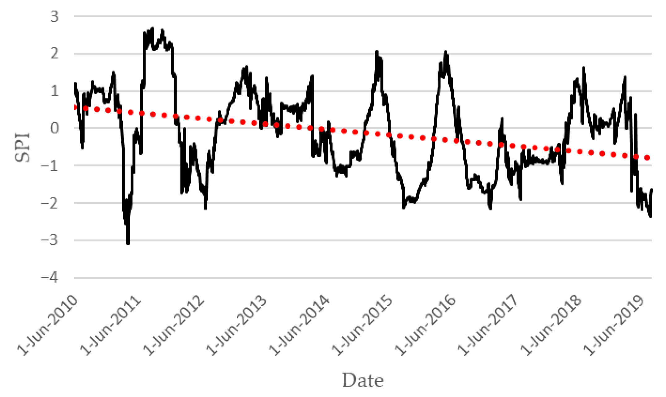
This study used data from Boryeong, Chungcheongnam-do, South Korea, which has experienced frequent meteorological droughts over the past 10 years. Boryeong is a coastal city located in the mid-west of South Korea, and Boryeong Dam supplies water to Chungcheongnam-do. Since 2012, a countermeasure committee has been established at the central government level due to drought. In particular, the annual rainfall decreased to 1010 and 785 mm during 2014–2015 due to severe drought. The subject area and precipitation measuring points can be observed in Figure 1, while the trend line for SPI6, which was the standard index consulted for drought warnings in Korea during the study period, is shown in Figure 2.

2.2. MLR

2.2.1. Developing the MLR Model

MLR is a statistical technique that expresses the relationship between several independent variables and a dependent variable, representing the linear relationship as a single functional formula. The principle is the same as that of the simple linear regression, which reveals the relationship between one independent variable and a dependent variable; however, the dependent variable is generally affected by more than two independent variables in terms of explaining the most natural phenomena. MLR was applied because the accuracy of the regression model could be improved by selecting several independent variables [20]. The MLR model, using one dependent variable ( y ) and several independent variables ( x i ), uses the form shown in Equation (1) as follows:
y = C + β 1 x 1 +   β 2 x 2 + β 3 x 3 β k x k ,
where β i ( i = 1 , 2 , k ) represents a regression coefficient for the independent variable x i ( i = 1 , 2 , k ) , y refers to the dependent variable, and C is the constant of the regression equation. The ordinary least squares method, which is commonly used when estimating regression coefficients, was used, and all independent variables used in the analysis were included in the regression equation by applying the simultaneous input method.

2.2.2. Model Assessment and Selection

The models developed by applying MLR analysis were evaluated in two ways. The first method measured the error of the SPI derived using each model in comparison with the actual SPI, while the second method compared the coefficient of determination of the derived regression equation. For the error evaluation index, the root mean squared error (RMSE) and mean absolute error (MAE) were calculated and compared. It has the characteristic of returning the error in a unit similar to that of the actual value. Regarding the RMSE, the square mean of the residuals of the estimated and actual values was calculated and square-rooted. RMSE is the most commonly used error evaluation index (Equation (2)). Compared to MAE, it has the characteristic of being sensitive to models with larger error values. MAE is the mean of the difference between actual and estimated values converted to an absolute value. It has an advantage over the RMSE when analyzing data with several outliers (Equation (3)).
R M S E = 1 m i = 1 m ( y i y ^ i ) 2
M A E = 1 m i = 1 m | y i y ^ i | ,
where m indicates the number of dataset days used for testing, and y i stands for the estimated value of the drought index for the applicable date obtained from the developed regression model. y ^ i denotes the actual drought index for that date. The coefficient of determination, which evaluates the performance of the derived regression model, and confirms its reliability, verifies the R2 and calculates adj.R2 (Equation (4)) values.
a d j . R 2 = 1 [ ( S S E ) ( n 1 ) n k 1 ( S S T ) ]
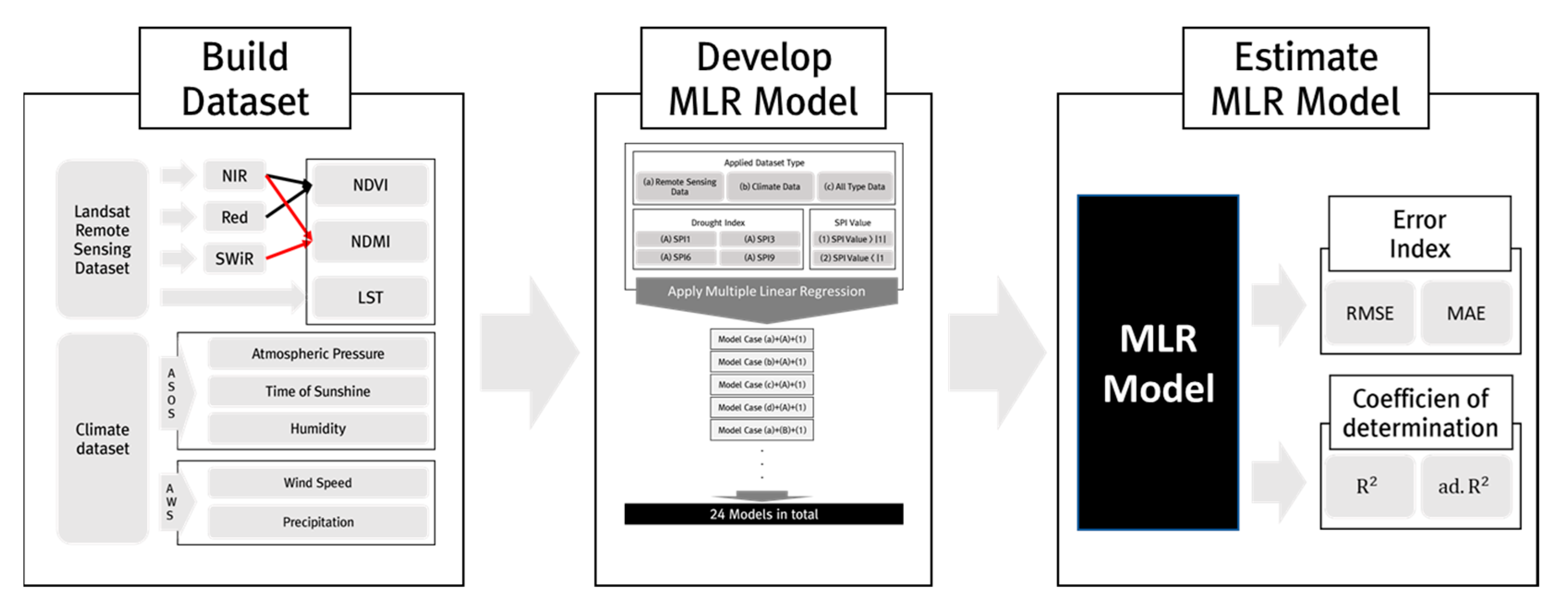
Here, SSE and SST are the sum of squares of error and total sum of squares of each model, n is the number of data, and k is the number of independent variable types R2 is an index that measures the degree to which the estimated linear model is suitable for the given data. It is generally interpreted as the explanatory power of the model, but increases as independent variables are added [21]; thus, when using MLR, R2 and adj.R2 were confirmed together. The 24 developed regression models were classified based on the SPI used as the dependent variable, and the performance of the models was compared. Figure 3 illustrates an overall schematic diagram of the research method.

2.3. Data

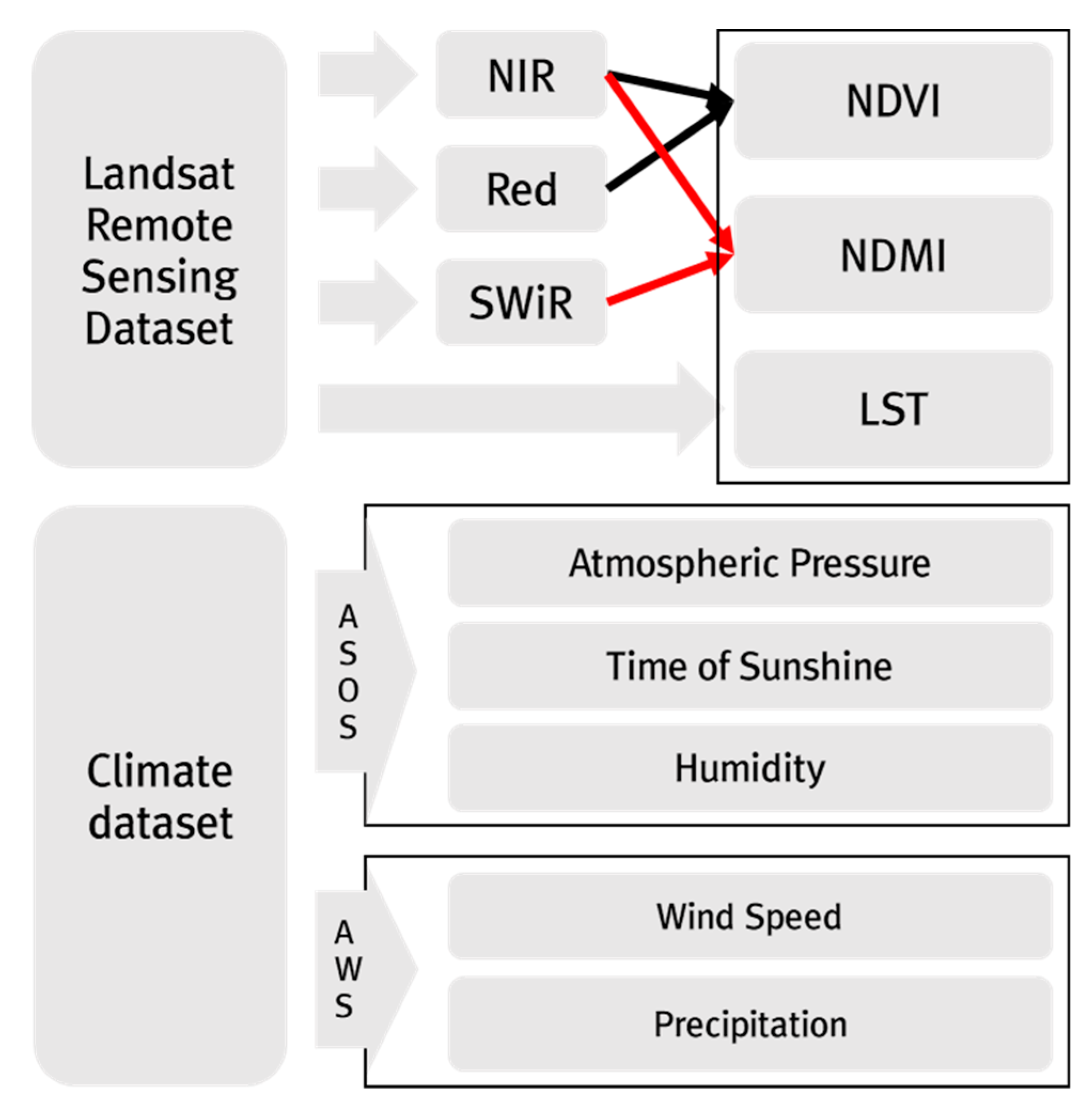
Drought index, satellite image data, and meteorological data were collected from reliable institutions to build a dataset to be used for the development of a MLR model. Drought index and meteorological data were collected from the Korea Meteorological Administration; satellite image data, i.e., Landsat 5 and Landsat 8 satellite images, were collected from the USGS. Subsequently, through QGIS, mean values for the three indices (NDVI, NDMI, and land surface temperature (LST)) used in determining drought were calculated. The raw data collated for this study have been itemized in Table 1.
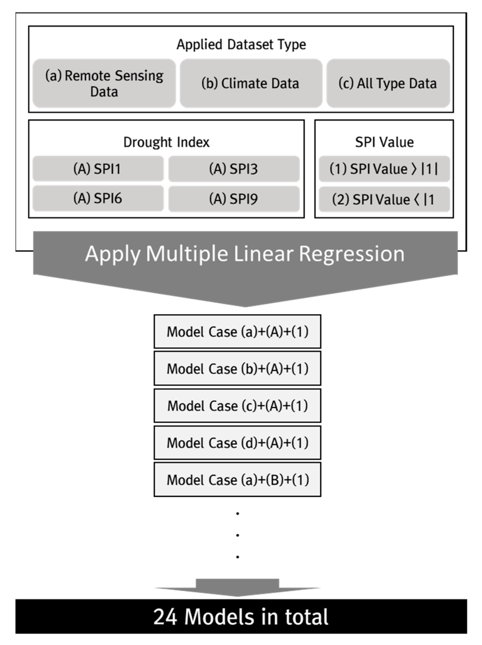
The study period was from June 2010 to September 2019, when droughts occurred frequently in Boryeong, and data were classified for a total of 76 days, facilitating their securement and development. We developed 24 models for this study by applying MLR analysis to each dataset and classifying them in groups of three, as shown in Figure 4. The SPI was used as the first classification criterion and was assigned as a dependent variable. Since four SPI types were used in this study (SPI1, SPI3, SPI6, and SPI9), there was a total of four cases.
The second classification criterion involved using the characteristics of the dataset, and this was applied as an independent variable. In this study, climate data, remote sensing data, or both were used as independent variables (all-type data). The study was conducted by dividing it into three data types, with the final classification being based on absolute SPI values, with cases divided into those with an absolute SPI value > 1 and those where it was < 1. We applied this distinction as the number of days when the SPI did not exceed 1 involved more than half of the built datasets. Moreover, in the evaluation stage, the performance of the regression model developed using undifferentiated data was rated as poor, owing to the data from dates with absolute SPI values > 1.
From data constructed in such a manner that the performance of the model could be evaluated more objectively, a model was developed by subjecting approximately 80% of the target period data to MLR analysis. For the rest, the performance was assessed by using values estimated through the model and comparing them with actual values. The number of days used for training each data classification and the testing dataset days are listed in Table 2.

2.3.1. Drought Indices

A drought index can express drought damage severity quantitatively, and several types have been developed to date. We used the drought index SPI as a dependent variable for regression model development. This drought index was developed using the idea that drought starts from a lack of precipitation [22]. It is the drought index most widely used to indicate drought severity. SPEI is a drought index that uses precipitation and evapotranspiration [23]; the method is similar to that of SPI, but is calculated by excluding cumulative evaporation from cumulative precipitation. Palmer expressed the depth of drought as a function of water shortage and the water shortage period via the Palmer Drought Severity Index (PDSI) [24]. Onyutha developed standardized non-parametric indices of precipitation and evaporation (SNIPE) The weakness of the drought index was compensated [25]. The drought index used as the dependent variable for regression model development is the Standardized Precipitation Index (SPI). In this study, four SPI types (SPI1, SPI3, SPI6, and SPI9) were collected, with the index number denoting the number of months (30 days per month) of cumulative precipitation used in its development. South Korea prepares its four weather drought warning stages using SPI6: mild drought (SPI6 < −1.0), moderate drought (<−1.5), severe drought (<−2.0), and extreme drought (<−2.0, lasting for >20 days). SPI is an index that expresses the optimal fit of precipitation to a probability distribution, and is one of the most widely used drought indices in modern times as suggested by Mckee et al. SPI is calculated using a standardized value of cumulative precipitation over a given period based on a 30 y precipitation record [26]. Because it has a variety of time scales, SPI is also used for drought monitoring, early warning, and drought severity estimation. Hydrological drought monitoring is possible with the use of a long-term SPI [27].

2.3.2. Climate Data

The data used as independent variables in this study were divided into two categories. The first type, point data measured at weather stations on the ground, were collected from two measuring platforms: automatic weather systems (AWSs) and automated synoptic observing systems (ASOSs). A total of 77 datasets was secured from June 2010 to June 2019 based on the date on which remote sensing data were collected. Average wind speed and daily precipitation data were collected from the AWS, which is an observation system involved in preventing natural disasters caused by weather phenomena such as typhoons, floods, and droughts. Based on the location of the AWS, a Thiessen polygon was created and replaced with the area data. ASOS is a ground observation system that is carried out simultaneously at all stations to determine the atmospheric conditions at a set time. It was used to collect certain weather elements that were not observed by the AWS, and the ASOS within Boryeong was selected. The ASOS data collected in this study were the local atmospheric pressure, average relative humidity, and average time of sunshine.

2.3.3. Remote Sensing Data

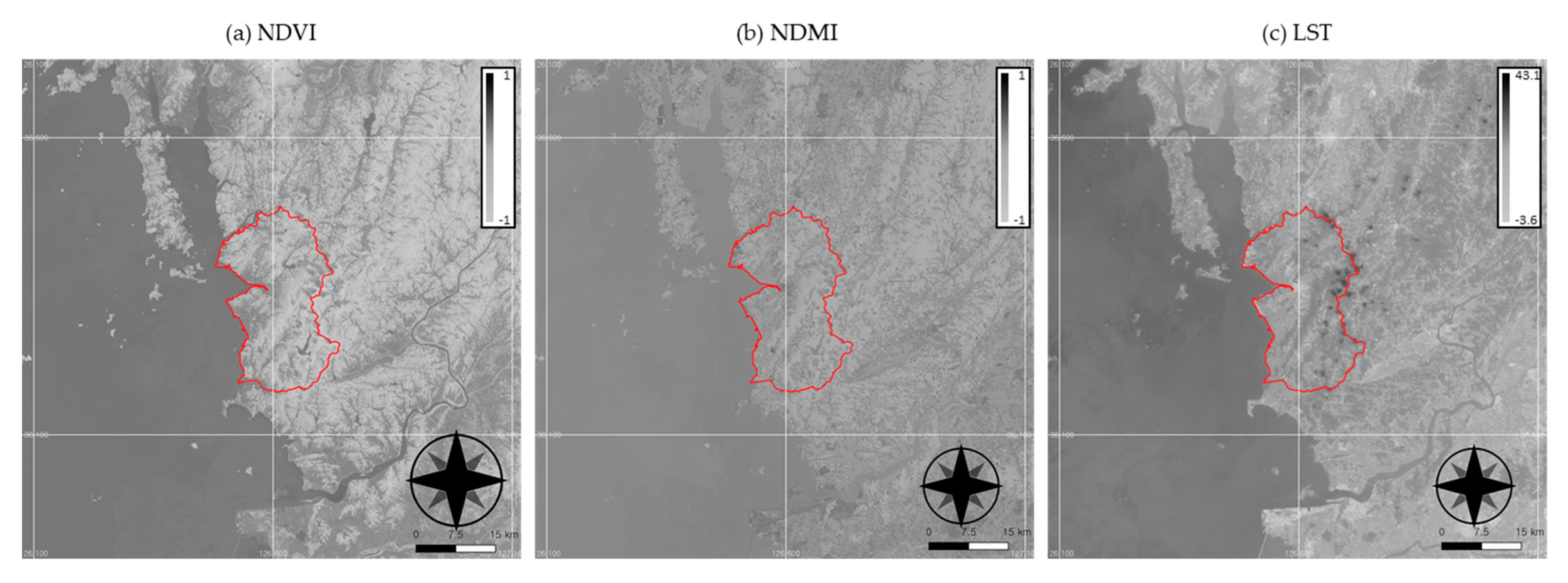
Remote sensing data refer to data collected remotely through satellites, and in this study, Landsat satellite imagery was used. The Landsat series of satellites supply photographic imagery covering the entire earth. These satellites were jointly developed by NASA and USGS, and eight satellites (Landsat 1 (1972) to Landsat 8 (2013)) have been launched in this series so far. Landsat satellite data are characterized by high quality and easy acquisition. They provide data in bands covering various wavelengths (see Table 3) and the required index can be calculated using this. For the collected satellite images, data on the days without cloud cover over Boryeong City were used from June 2010 to June 2019. The band types provided by each satellite can be verified through Table 3. The index used as an independent variable can be calculated using the Landsat bands required for NDVI, NDMI, and LST. Figure 5 shows the remote sensing data of Boryeong on 13 June 2019, which were obtained from Landsat satellite images. In this study, the three area-averaged indicators—NDVI, NDMI, and LST—were computed using Landsat 5 and Landsat 8 satellite imagery.
NDVI analyzes the difference between the reflectance at the near-infrared (NIR) and red wavelengths and is the most widely used vegetation-related index. In a healthy vegetation area, the red wavelength is absorbed and the near-infrared wavelength has a high reflectance. Conversely, in the case of soil without vegetation, the reflectance in the red region is high, but that in the near-infrared region is low [28]. To emphasize this characteristic, the NDVI—which ranges from 1 to −1, with a higher value indicating healthy vegetation—is denoted as shown in Equation (5) below:
NDVI = N e a r   i n f r a r e d R e d N e a r   i n f r a r e d + R e d ( = B a n d 5 B a n d 4 B a n d 5 + B a n d 4 i n   L a n d s a t   8 , B a n d 4 B a n d 3 B a n d 4 + B a n d 3 i n   L a n d s a t   5 )
NDMI is used to determine vegetation moisture content. It focuses on removing changes due to the leaf’s internal structure and dry matter content in the vegetated area and explores vegetation moisture content by highlighting the difference between NIR and short-wavelength infrared (SWIR) measurements. The reflectance of SWIR is inversely proportional to the moisture content of the leaf, and the NDMI is represented as shown in Equation (6) below:
NDMI = N e a r   i n f r a r e d s h o r t   w a v e   i n f r a r e d N e a r   i n f r a r e d + s h o r t   w a v e   i n f r a r e d ( = B a n d 5 B a n d 6 B a n d 5 + B a n d 6 i n   L a n d s a t   8 ,   B a n d 4 B a n d 5 B a n d 4 + B a n d 5 i n   L a n d s a t   5 )
Landsat provides the amount of energy observed for each channel, which is used to calculate LST data for that digit number (DN). For LST calculation, the data were converted into the actual amount of radiation through an equation provided by the USGS [29]. Landsat 5’s LST was calculated by substituting Equation (7) for Band 6, and for Landsat 8, LST was calculated by substituting Equation (8) for Bands 10 and 11.
L λ = [ L M a x λ L M i n λ Q c a l m a x Q C a l m i n ] × [ Q c a l Q c a l m i n ] + L m i n λ ,
where L λ is the spectral radiation amount reaching the sensor, Q c a l shows the DN of the pixel unit analyzed in the image data, L M i n λ represents the spectral radiation amount when Q c a l is zero, and L M a x λ denotes the spectral radiation amount when Q c a l = Q c a l m a x . Q c a l m a x and Q C a l m i n are the values expressed in DN units after quantifying the minimum and maximum radiation amounts, respectively.
L λ = M L × Q c a l + A L
where L λ represents the amount of spectral radiation reaching the sensor, and M L is the radiance multiplicative scaling factor for the band. Q c a l represents the DN value of the pixel, and A L denotes the radiance additive scaling factor for the band. The radiation calculation was used to determine the “brightness” temperature, as shown in Equation (9) below:
T = K 2 ln ( K 1 L λ + 1 ) ,
where T indicates the brightness temperature (K), and coefficients K 1 and K 2 (as Watts / ( m 2 · srad · μ m )) represent correction factors provided by the USGS, as shown in Table 4. In this study, Landsat 8 Band 10 data were used for LST calculations.
We also needed to calculate the emission rate ( ε ), which was determined as shown in Table 5 using the NDVI range. The USGS recommends not relying on values calculated using Landsat 8 Band 11 for LST calculation due to its higher levels of uncertainty; therefore, in this study, LST was calculated using data from Band 10 only [30].
Finally, LST values were calculated using a plugin provided by QGIS, which applied Equation (10) provided below (unit: K):
LST =   ε 1 4 T
The construction process applied to create each dataset has been illustrated in the schematic shown in Figure 6.

3. Results

3.1. MLR Model Development

3.1.1. Coefficient of Determination

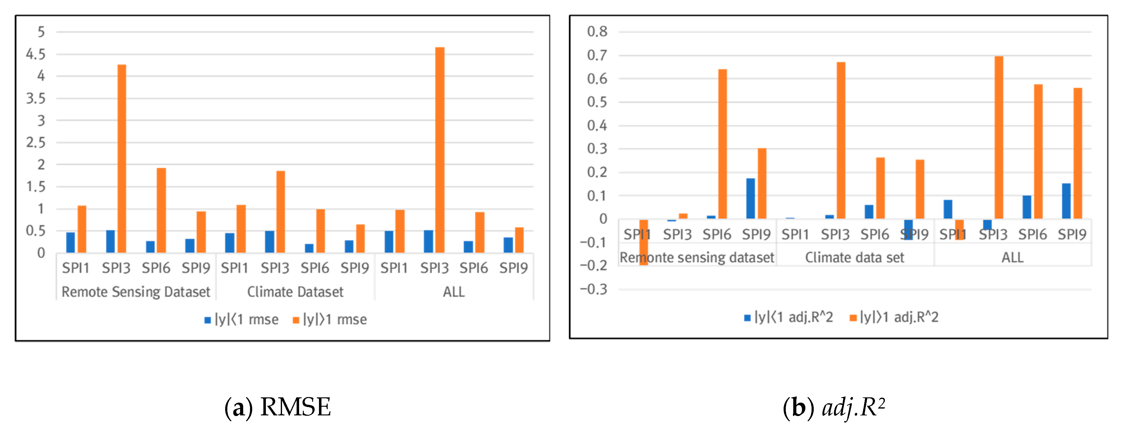
The SPI value was estimated using each of the constructed MLR models. Table 6 presents the coefficients of the regression model developed by applying the previously suggested method to the all-type dataset. The t-value indicates the significance of each coefficient; the larger the absolute value, the greater the significance. The overall model summary, where R2 and adj.R2 values were verified, is presented in Table 7 and Each case with the highest coefficient of determination of the drought index was shaded. The F-value indicates the significance of the regression equation, and the larger the value, the greater the significance. The models with | y ^ | > 1 exhibited higher adj.R2 values than those with | y ^ | < 1 in general, and datasets with more variables had more significance.
However, there were exceptions. First, SPI1 did not markedly vary across most models. The adj.R2 value of the | y ^ | > 1 ( = −0.00062) model was low at −0.19763. Moreover, SPI6 of the | y ^ | > 1 model (the remote sensing dataset), which used the least independent variables, had the highest adj.R2 value at 0.64204. In the | y ^ | > 1 model, the adj.R2 value for SPI3, which used all the variables, was the highest at 0.695654. The | y ^ | > 1 for the same drought index and climate dataset model had the second-highest value at 0.672715; however, the adj.R2 value for the | y ^ | < 1 model was low, and this poor performance indicated that it was not reasonable to use a regression model that achieved such results.

3.1.2. RMSE and MAE

RMSEs and MAEs were calculated and compared to evaluate the drought index estimation ability of the models developed in this study. As the R2 and adj.R2 values of |SPI| < 1 were not satisfactory, a model with different criteria needed to be selected to present the regression equation in this case. The RMSE and MAE, which are used as error indicators, were applied to calculate the comparative residuals between the estimated and actual SPI values calculated using the developed model. Table 8 shows the RMSE and MAE of each model, and the error evaluation indicators with the best performance were shaded. All the error indicators had values lower than the | y ^ | < 1 dataset, which indicated that using | y ^ | < 1 would result in better estimations.
The | y ^ | < 1 climate dataset demonstrated better estimation ability than other dataset types, and SPI6 had the lowest RMSE and MAE of all the indices. Furthermore, the | y ^ | < 1 dataset performed better in the SPI6 and SPI9 models, which have been used to determine drought using relatively long-term rainfall data, than it did in the SPI1 and SPI3 models, which use short-term precipitation data. In fact, SPI9 had the highest estimation ability of the indices using the | y ^ | < 1 climate dataset, followed by SPI1, SPI6, and SPI3. However, notably, the R2 and adj.R2 values of the SPI1 model were unsatisfactory.

3.1.3. Best Model Selection

The size of adj.R2 was selected as a criterion, based on the results shown in Table 8, for the | y ^ | > 1 models, while for the | y ^ | < 1 models, RMSEs were compared, with low values being preferred. A graph comparing the adj.R2 and RMSE values calculated for each model is shown in Figure 7, with the regression model for each SPI considered in this study presented in Table 9 and notable results were shaded.
These results showed that all | y ^ | < 1 models had their lowest RMSE when only the climate dataset was used and that the remote sensing data did not significantly influence their SPI estimate results. With respect to the | y ^ | > 1 models selected using adj.R2 values, all models that used the remote sensing data performed satisfactorily, except for SPI1. Thus, models that used only the remote sensing data were selected for SPI6. Our results showed that the SPI3 and SPI6 models had high adj.R2 values compared to other models. However, their RMSEs were lower than those of the other models, and the RMSE calculated for the SPI3 | y ^ | > 1 model being the highest at 4.65. SPI9 had the best performance when estimation ability of the model was assessed using RMSEs. In addition, unlike other models with a value >1, the SPI9 | y ^ | > 1 model had high adj.R2 and low RMSE values. However, the fact that the adj.R2 value of the SPI9 | y ^ |>1 model was the lowest among the selected models had to be taken into account.

4. Discussion

This study developed an MLR model and evaluated the possibility of using Landsat remote sensing data to compensate for the weakness of the existing research that estimates only a very small range of drought. To evaluate the applicability of remote sensing data for drought estimation, we extracted data to be used in drought indices from Landsat satellite imagery covering Boryeong, and developed a model for the application of MLR analyses. Most of the | y ^ | > 1 model results, excluding SPI1, yielded a higher adj.R2 than the models using remote sensing and climate data. Thus, remote sensing data are expected to be effective when estimating the lack of accumulated precipitation for 3–6 months. However, the results of this study revealed limitations. First, among the models using remote sensing data, the models with SPI1 as the dependent variable showed poor overall performance. NDVI and NDMI included in the remote sensing dataset type are affected by vegetation and soil moisture, respectively, and these indices are also affected by long-term meteorological phenomena [31]. We found that the differences between the coefficients of determination and error indices were large and related to the range of | y ^ |. For the constructed datasets, Landsat satellite imagery data were collected for cloudless days over Boryeong, rather than at regular intervals. This approach—in addition to the fact that a Landsat satellite only observes the same area for approximately 16 days [32]—made building data using regular intervals difficult. [33] Consequently, accounting for the weather between dates established using only the SPI and remote sensing data was difficult. The use of TERRA/AQUA MODIS data—which are updated on a daily basis—or GEO-KOMPSAT satellite imagery—which continually observes only Korea—would have achieved satisfactory performance regardless of the | y ^ | range. Based on this research methodology, a more diverse model should be developed and applied to other regions of similar size. It will then be possible to expand the research results by applying a more versatile model to national (and continental) scale units. Notably, SPI is calculated using cumulative precipitation, although NDVI and NDMI are more related to soil moisture, suggesting the need for a follow-up study that examines a drought index other than the SPI as an independent variable. This follow-up study may apply indices selected based on their ability to estimate agricultural or hydrological drought, moving beyond simple meteorological drought estimation. Lastly, the results of this study suggest that the application of deep learning (rather than machine learning) techniques, such as MLR analysis, can improve performance and nonlinear expressiveness, resulting in the development of more accurate and reliable models. [34]. Based on this research methodology, a more diverse model should be developed and applied to other regions of a similar size to expand the research results by developing a highly versatile model through application to entire countries and continents.

5. Conclusions

Water shortages can be addressed and drought-related damage minimized by estimating drought and establishing countermeasures in advance. An important task in water resource management is preparing for extreme drought in the near future by exploring satellite remote sensing data that are suitable for drought estimation research, and creating methodology that can develop better models based on research results.

Author Contributions

Data curation, S.W.K.; methodology, S.W.K. and Y.-J.C.; project administration, D.J. and Y.-J.C.; supervision, D.J. and Y.-J.C.; writing—original draft, S.W.K.; writing—review and editing, D.J. and Y.-J.C. All authors have read and agreed to the published version of the manuscript.

Funding

This research was supported by a grant (2019-MOIS31-010) from the Fundamental Technology Development Program for Extreme Disaster Response, funded by the Korean Ministry of Interior and Safety (MOIS).

Conflicts of Interest

The funders had no role in the design of the study; in the collection, analyses, or interpretation of data; in the writing of the manuscript, or in the decision to publish the results.

References

  1. Hong, M.; Kim, J.; Jung, G.; Jeong, S. Rainfall Threshold (ID Curve) for Landslide Initiation and Prediction Considering Antecedent Rainfall. Korean Geotech. Soc. 2016, 32, 15–27. [Google Scholar] [CrossRef] [Green Version]
  2. Mohammad, V. How Do Different Factors Impact Agricultural Water Management? Open Agric. 2016, 1, 89–111. [Google Scholar]
  3. Mohammad, V. Global Experience on Irrigation Management Under Different Scenarios. J. Water Land Dev. 2017, 32, 95–102. [Google Scholar]
  4. Weili, D.; Naota, H.; Hideo, S.; Yaning, C.; Shan, Z.; Daniel, N.; Botao, Z.; Yi, W. Evaluation and Future Projection of Chinese Precipitation Extremes Using Large Ensemble High-Resolution Climate Simulations. J. Clim. 2019, 32, 2169–2183. [Google Scholar]
  5. Shan, Z.; Jilili, A.; Jianli, D.; Weili, D.; Philippe, M.D.; Tim, D.V.V. Description and Attribution Analysis of the 2017 Spring Anomalous High Temperature Causing Floods in Kazakhstan. J. Meteorol. Soc. Jpn. 2020, 2, 70. [Google Scholar] [CrossRef]
  6. Weili, D.; Bin, H.; Kaoru, T.; Pingping, L.; Maochuan, H.; Nor, E.A.; Daniel, N. Changes of Precipitation Amounts and Extremes Over Japan Between 1901 and 2012 and Their Connection to Climate Indices. Clim. Dyn. 2015, 45, 2273–2292. [Google Scholar]
  7. Mohammad, V.; Sayed, M.B.; Mohammad, A.G.S.; Mahmoud, R.S.; Vijay, P.S. Complexity of Forces Driving Trend of Reference Evapotranspiration and Signals of Climate Change. Atmosphere 2020, 11, 1081. [Google Scholar]
  8. Eom, J.; Park, S.; Ko, B.; Lee, C. Monitoring of Lake Area Change and Drought Using Landsat Images and the Artificial Neural Network Method in Lake Soyang, Chuncheon, Korea. J. Korean Earth Sci. Soc. 2020, 41, 129–136. [Google Scholar] [CrossRef]
  9. Ye, Z.; Yi, L.; Xieyao, M.; Liliang, R.; Vijay, P.S. Drought Analysis in the Yellow River Basin Based on a Short-Scalar Palmer Drought Severity. Water 2018, 10, 1526. [Google Scholar]
  10. Alex, A.; Rolando, C.; Abel, S.; Javier, P. Probabilistic prediction of drought events using Markov Chain and Bayesian network-based models: A case study of the Andean regulatory river basin. Water 2016, 8, 37. [Google Scholar]
  11. Ji, L.; Peters, A.J. Assessing Vegetation Response to Drought in the Northern Great Plains Using Vegetation and Drought Indices. Remote Sens. Environ. 2003, 87, 85–98. [Google Scholar] [CrossRef]
  12. Thomas, B.F.; Famiglietti, J.S.; Landerer, F.W.; Wiese, D.N.; Molotch, N.P.; Argus, D.F. Grace Groundwater Drought Index: Evaluation of California Central Valley Groundwater Drought. Remote Sens. Environ. 2017, 198, 384–392. [Google Scholar] [CrossRef]
  13. Mu, Q.; Zhao, M.; Kimball, J.S.; McDowell, N.G.; Running, S.W. A Remotely Sensed Global Terrestrial Drought Severity Index. Bull. Am. Meteorol. Soc. 2013, 94, 83–98. [Google Scholar] [CrossRef] [Green Version]
  14. Een-Sook, K.; Bora, L.; Jong-Hwan, L. Forest Damage Detection Using Daily Normal Vegetation Index Based on Time Series LANDSAT Images. Korean J. Rem. Sens. 2019, 35, 1133–1148. [Google Scholar]
  15. Jianzhu, L.; Shuhan, Z.; Ro’ng, H. Hydrological Drought Class Transition Using SPI and SRI Time Series by Loglinear Regression. Water Resour. Manag. 2015, 30, 669–684. [Google Scholar]
  16. Zhang, R.; Chen, Z.Y.; Xu, L.J.; Ou, C.Q. Meteorological Drought Forecasting Based on a Statistical Model With Machine Learning Techniques in Shaanxi Province, China. Sci. Total Env. 2019, 665, 338–346. [Google Scholar] [CrossRef]
  17. Kang, K.; Jeung, S.J.; Lee, S.; Kim, B. Evaluation of long-term runoff model in unmeasured watershed using satellite data; Focusing on the Imjin River basin. In Proceedings of the 2015 Korea Water Resources Association Annual Conference, Goseong, Korea, 28–29 May 2015. [Google Scholar]
  18. Peng, F.; Qihao, W. Consistent land surface temperature data generation from irregularly spaced Landsat imagery. Remote Sen. Environ. 2016, 184, 175–187. [Google Scholar] [CrossRef]
  19. Mun, Y.; Nam, S.W.; Kim, H.; Hong, T.E.; Sur, M.C. Evaluation and comparison of meteorological drought index using multi-satellite based precipitation products in East Asia. J. Kor. Soc. Agric. Eng. 2020, 62, 83–93. [Google Scholar]
  20. Yun, H.; Um, M.; Cho, W.; Heo, J.H. Orographic Orographic Precipitation Analysis with Regional Frequency Analysis and Multiple Linear Regression. J. Korea Water Resour. Assoc. 2009, 42, 465–480. [Google Scholar] [CrossRef] [Green Version]
  21. Choi, S.; Han, Y.K.; Kim, Y.B. Comparison of Different Multiple Linear Regression Models for Real-Time Flood Stage Forecasting. J. Korean Soc. Civ. Eng. 2012, 32, 9–20. [Google Scholar]
  22. McKee, T.B.; Doesken, N.J.; Kleist, J. The Relationship of Drought Frequency and Duration of Time Scales. In Proceedings of the 8th Conference on Applied Climatology, Anaheim, CA, USA, 17–23 January 1993; pp. 179–186. [Google Scholar]
  23. Sergio, M.V.S.; Santiago, B.; Juan, I.L.M. A Multiscalar Drought Index Sensitive to Global Warming: The Standardized Precipitation Evapotranspiration Index. J. Clim. 2010, 23, 1696–1718. [Google Scholar]
  24. Palmer, W.C. Meteorological Drought; Department of Commerce Weather Bureau Research: Washington, DC, USA, 1965; Volume 30. [Google Scholar]
  25. Onyutha, C. On Rigorous Drought Assessment Using Daily Time Scale: Non-Stationary Frequency Analyses, Revisited Concepts, and a New Method to Yield Non-Parametric Indices. Hydrology 2017, 4, 48. [Google Scholar] [CrossRef] [Green Version]
  26. Tommaso, C.; Simone, V.; Paola, C.; Francesco, F. Drought Analysis in Europe and in the Mediterranean Basin Using the Standardized Precipitation Index. Water 2018, 10, 1043. [Google Scholar]
  27. Lang, X.; Fen, Z.; Kebiao, M.; Zijin, Y.; Zhiyuan, Z.; Tongren, X. SPI-Based Analyses of Drought Changes over the Past 60 Years in China’s Major Crop-Growing Areas. Remote Sens. 2018, 10, 171. [Google Scholar]
  28. Rouse, J.W.; Haas, R.H.; Schell, J.A.; Deering, D.W. Monitoring Vegetation Systems in the Great Plains With ERTS. In Proceedings of the 3rd Earth Resource Technology Satellite-1 Symposium, Washington, DC, USA, 10–14 December 1974; Volume 1, pp. 48–62. [Google Scholar]
  29. Landsat Project Science Office Landsat 8 Science Data User’s Handbook. Available online: http://www.gsfc.nasa.gov/IAS/handbook/handbook_toc.html (accessed on 5 December 2019).
  30. Kim, G.H.; Hong, S.O.; Kim, D.H.; Park, H.S.; Lee, Y.G.; Kim, B.C. Calculation of Surface Temperature Using Landsat 8 Satellite Data and Analysis of Urban. Greening Effect; Meteorological Application Research Laboratory National Institute of Meteorological Sciences: Jeju, Korea, 2016. [Google Scholar]
  31. Sekertekin, A.; Bonafoni, S. Land Surface Temperature Retrieval from Landsat 5, 7, and 8 over Rural Areas: Assessment of Different Retrieval Algorithms and Emissivity Models and Toolbox Implementation. Remote Sens. 2020, 12, 294. [Google Scholar] [CrossRef] [Green Version]
  32. Peterson, K.T.; Sagan, V.S.; Sidike, P.; Cox, A.L.; Martinez, M. Suspended Sediment Concentration Estimation from Landsat Imagery along the Lower Missouri and Middle Mississippi Rivers Using an Extreme Learning Machine. Remote Sens. 2018, 10, 1503. [Google Scholar] [CrossRef] [Green Version]
  33. Hao, P.; Löw, F.; Biradar, C. Annual Cropland Mapping Using Reference Landsat Time Series—A Case Study in Central Asia. Remote Sens. 2018, 10, 2057. [Google Scholar] [CrossRef] [Green Version]
  34. Huang, X.; Gao, L.; Crosbie, R.S.; Zhang, N.; Fu, G.; Dobble, R. Groundwater Recharge Prediction Using Linear Regression, Multi-Layer Perception Network, and Deep Learning. Water 2019, 11, 1879. [Google Scholar] [CrossRef] [Green Version]
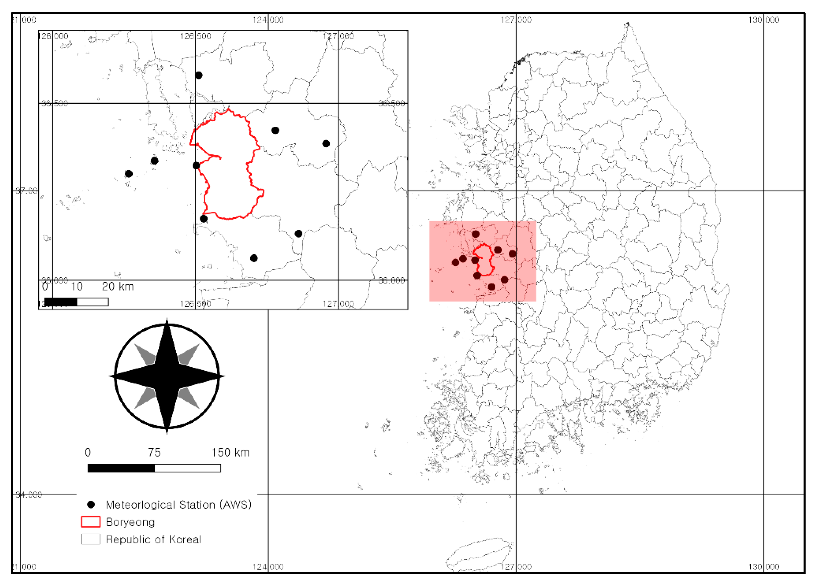
Figure 1. Location within the Republic of Korea and automatic weather system sites around Boryeong.
Water 12 03393 g001
Figure 2. Boryeong SPI6 time-series, with fitted linear regression.
Water 12 03393 g002
Figure 3. Model development process.
Water 12 03393 g003
Figure 4. Model development process.
Water 12 03393 g004
Figure 5. Remote sensing data for Boryeong on 13 July 2019.
Water 12 03393 g005
Figure 6. Dataset building process.
Water 12 03393 g006
Figure 7. Evaluation results achieved by each model.
Water 12 03393 g007
Table 1. Raw data summary.
Data TypeNameSource
Drought indexSPI1Korea Meteorological Administration
SPI3
SPI6
SPI9
Climate dataAtmospheric pressure
Hours of sunshine
Humidity
Wind speed
Precipitation
Remote sensing dataLandsat 5United States Geological Survey
Landsat 8
Table 2. Dataset days used for developing each model.
Drought Indexabs(x) < 1abs(x) > 1Data Used
Training
(Days)
Testing
(Days)
Total
(Days)
Training
(Days)
Testing
(Days)
Total
(Days)
SPI1371047 (61.8%)23629 (38.2%)76
(100%)
SPI3441155 (72.3%)17421 (27.7%)
SPI6411051 (67.1%)20525 (32.9%)
SPI9391049 (64.5%)21627 (35.5%)
Table 3. Bands provided by Landsat 5 and Landsat 8.
SpectralWavelengthResolutionLandsat 5Landsat 8
Coastal/aerosol0.43–0.4530 mXBand 1
Band 2—Blue0.45–0.5130 mBand 1Band 2
Band 3—Green0.53–0.5930 mBand 2Band 3
Band 4—Red0.64–0.6730 mBand 3Band 4
Band 5—Near infrared0.85–0.8830 mBand 4Band 5
Band 6—Shortwave infrared (1)1.57–1.6530 mBand 5Band 6
Band 7—Shortwave infrared (2)2.11–2.2930 mBand 7Band 7
Band 8—Panchromatic0.5–0.6815 mXBand 8
Band 9—Cirrus1.36–1.3830 mXBand 9
Band 10—Thermal wave infrared (1)10.6–11.1930 mBand 6Band 10
Band 11—Thermal wave infrared (2)11.5–12.5130 mBand 11
Table 4. K coefficients.
K 1 K 2
Band 6 in Landsat 5607.761260.56
Band 10 in Landsat 8774.891321.08
Band 11 in Landsat 8480.891201.14
Table 5. Emissivity according to the normalized difference vegetation index (NDVI).
NDVI Ranges Emissivity   ( ε )
NDVI < −0.1850.995
−0.185 < NDVI < 0.1570.970
0.157 < NDVI < 0.7271.0994 + 0.047 ln (NDVI)
0.727 < NDVI0.990
Table 6. Multiple linear regression (MLR) regression coefficients achieved using the all-type dataset as input.
Drought Index | y ^ | < 1 | y ^ | > 1
NameBtNameβt
SPI1 C 30.935781.869993 C 3.2014590.040555
NDVI−0.72796−0.57769NDVI10.36281.290699
NDMI−0.53576−0.42926NDMI−0.8802−0.15897
LST−0.02705−1.24816LST−0.1316−1.13698
Humidity0.0011360.132262Humidity−0.02991−0.51526
Atmospheric pressure−0.03019−1.89291Atmospheric pressure−0.00544−0.07237
Hours of sunshine0.0125330.552531Hours of sunshine0.0668980.586851
Precipitation−0.02082−1.3711Precipitation0.8306781.816239
Wind speed0.0092830.258267Wind speed1.1608232.029992
SPI3 C 12.909110.836061 C 188.10640.896862
NDVI0.9506190.641093NDVI11.734261.403033
NDMI−0.71064−0.4874NDMI−9.47014−1.83521
LST−0.01654−0.81279LST−0.2059−1.37255
Humidity0.0024490.299923Humidity−0.04421−0.36255
Atmospheric pressure−0.01319−0.88639Atmospheric pressure−0.18753−0.94184
Hours of sunshine0.0296071.413231Hours of sunshine0.3009783.479056
Precipitation0.0085840.56126Precipitation1.4001662.694312
Wind speed−0.01367−0.4086Wind speed−0.12401−0.13981
SPI6 C −17.8702−0.94269 C −22.093−0.3271
NDVI1.8858111.142978NDVI1.2108220.362712
NDMI−1.66831−1.25147NDMI−16.4954−2.84382
LST−0.05058−2.05796LST0.2060922.408501
Humidity0.0100771.062627Humidity−0.02773−0.9022
Atmospheric pressure0.016830.923181Atmospheric pressure0.0226460.348437
Hours of sunshine0.0299991.324477Hours of sunshine0.0604880.867988
Precipitation−0.01364−0.79141Precipitation0.0412490.197038
Wind speed0.0799581.983995Wind speed0.0432330.174417
SPI9 C 20.355911.187025 C 150.9162.859393
NDVI−2.10529−1.19325NDVI10.677313.764342
NDMI2.7558882.25374NDMI−9.92022−2.10782
LST−0.0162−0.63835LST−0.17683−2.56174
Humidity−0.01264−1.39552Humidity−0.01482−0.60831
Atmospheric pressure−0.01872−1.13645Atmospheric pressure−0.14861−2.88596
Hours of sunshine−0.01061−0.53462Hours of sunshine−0.00033−0.0061
Precipitation0.006950.453522Precipitation0.1599751.010333
Wind speed−0.06159−0.9094Wind speed0.2134452.516916
Table 7. Coefficients of determination.
MLR Model Type | y ^ | < 1 | y ^ | > 1
R2adj.R2FR2adj.R2F
Remote sensing datasetSPI10.083−0.0010.9930.042−0.1980.175
SPI30.060−0.0100.8530.3180.0251.086
SPI60.0900.0161.2190.6990.64212.360
SPI90.2400.1753.6870.4030.3034.048
Climate datasetSPI10.1430.0051.0380.3360.0031.010
SPI30.1320.0181.1570.8360.6735.111
SPI60.1790.0621.5280.4580.2652.369
SPI90.054−0.0890.3780.4320.2542.434
ALLSPI10.2860.0821.0380.491−0.0900.993
SPI30.149−0.0461.1570.9390.6963.857
SPI60.2820.1021.5280.7550.5772.369
SPI90.3320.1540.3780.7290.5624.366
Table 8. Root mean squared error (RMSE) and mean absolute error (MAE) for each multi-linear model.
Dataset TypeDrought Index | y ^ | < 1 | y ^ | > 1
RMSEMAERMSEMAE
Remote sensing datasetSPI10.4610630.3701681.0728390.849006
SPI30.5239660.4166564.2674514.104682
SPI60.271080.1882831.9235011.811254
SPI90.329290.2774750.949530.783517
Climate datasetSPI10.4529230.371941.0880431.075702
SPI30.4970070.4164311.8621511.633461
SPI60.2030240.1558760.9925780.972057
SPI90.2883970.2084150.6565230.51566
AllSPI10.4966790.3664670.984490.829243
SPI30.5127420.4208624.6496674.220784
SPI60.2783930.1575710.9283450.907182
SPI90.3521820.2903290.5808240.4903
Table 9. Results used to select the best model (N/V = no value).
| y ^ | < 1 | y ^ | > 1
Badj.R2RMSEβadj.R2RMSE
SPI1 C 12.85730.0053070.45292312.85730.0033381.088043
Humidity0.0012610.001261
Atmospheric pressure−0.01282−0.01282
Hours of sunshine0.0212960.021296
Precipitation−0.03012−0.03012
Wind speed−0.01179−0.01179
SPI3 C 13.440630.0179540.497007188.10640.6956544.649667
NDVI(N/V)11.73426
NDMI(N/V)−9.47014
LST(N/V)−0.2059
Humidity0.000101−0.04421
Atmospheric pressure−0.01355−0.18753
Hours of sunshine0.0327140.300978
Precipitation0.0065081.400166
Wind speed−0.03087−0.12401
SPI6 C −20.85310.0619020.203024−0.162860.642041.923501
NDVI(N/V)2.309607
NDMI(N/V)−17.988
LST(N/V)0.160818
Humidity0.003844(N/V)
Atmospheric pressure0.02011(N/V)
Hours of sunshine0.034192(N/V)
Precipitation−0.02157(N/V)
Wind speed0.027265(N/V)
SPI9 C 8.405069−0.089180.288397150.9160.5618340.580824
NDVI(N/V)10.67731
NDMI(N/V)−9.92022
LST(N/V)−0.17683
Humidity−0.0089−0.01482
Atmospheric pressure−0.00744−0.14861
Hours of sunshine−0.01545−0.00033
Precipitation0.0045970.159975
Wind speed−0.036520.213445
Publisher’s Note: MDPI stays neutral with regard to jurisdictional claims in published maps and institutional affiliations.