Wave Interaction and Overwash with a Flexible Plate by Smoothed Particle Hydrodynamics


Abstract
:1. Introduction
2. Wave Generation
3. sph
3.1. Fluid Phase
3.2. Solid Phase
3.3. Free Surface
4. Results
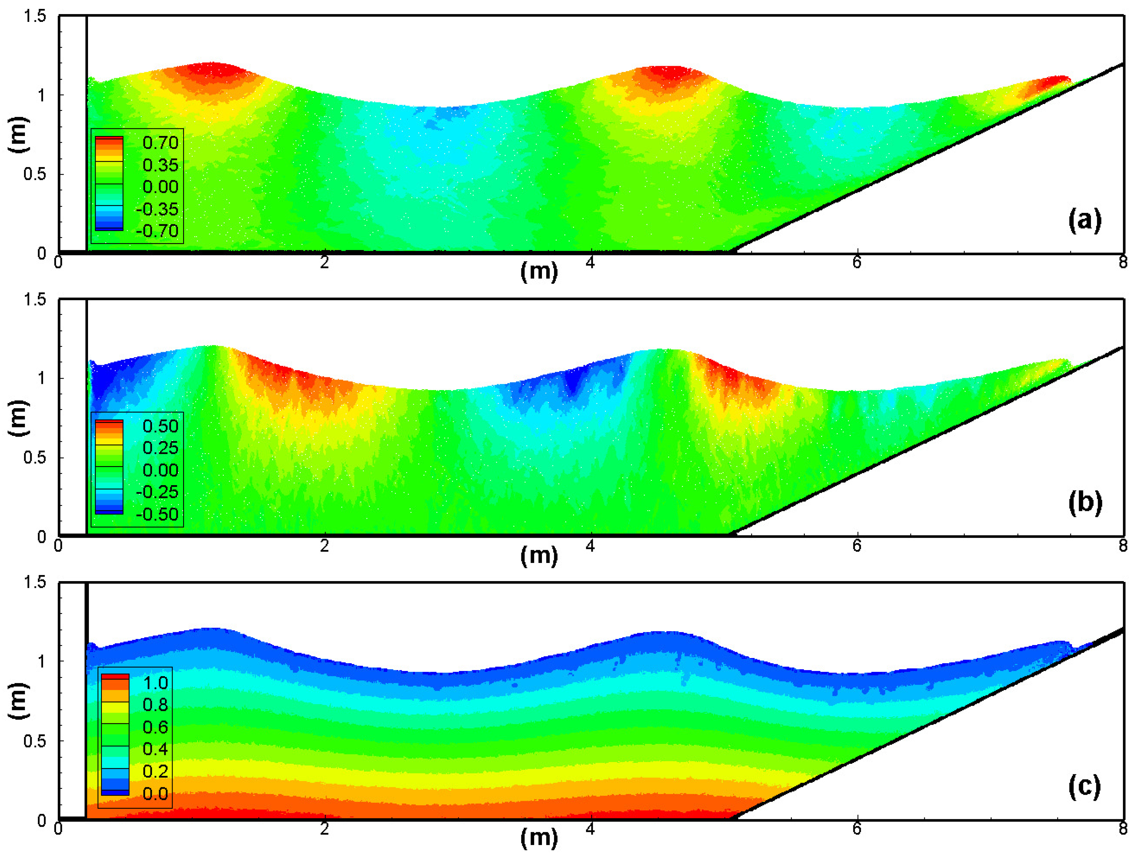
4.1. Waves
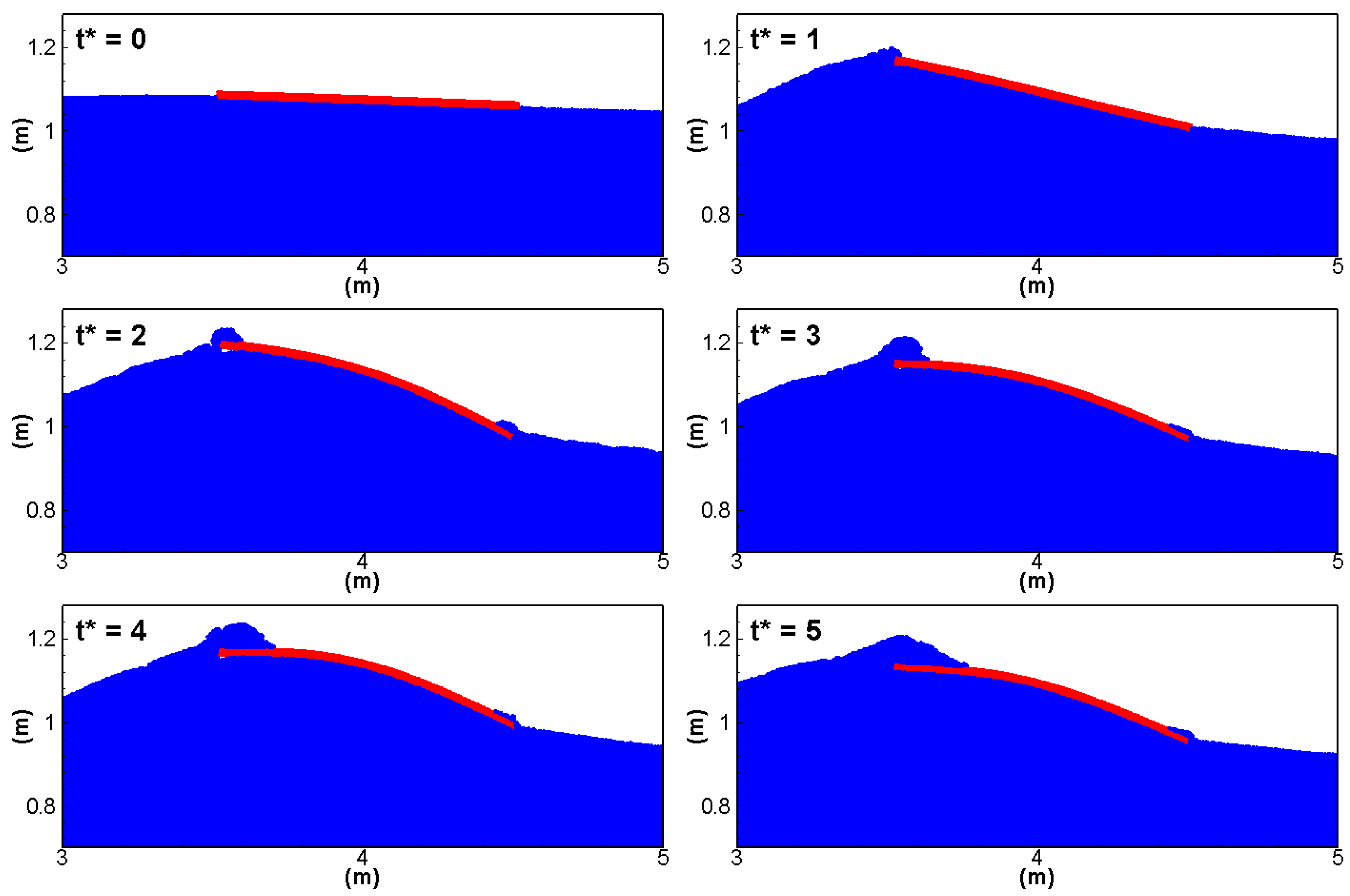
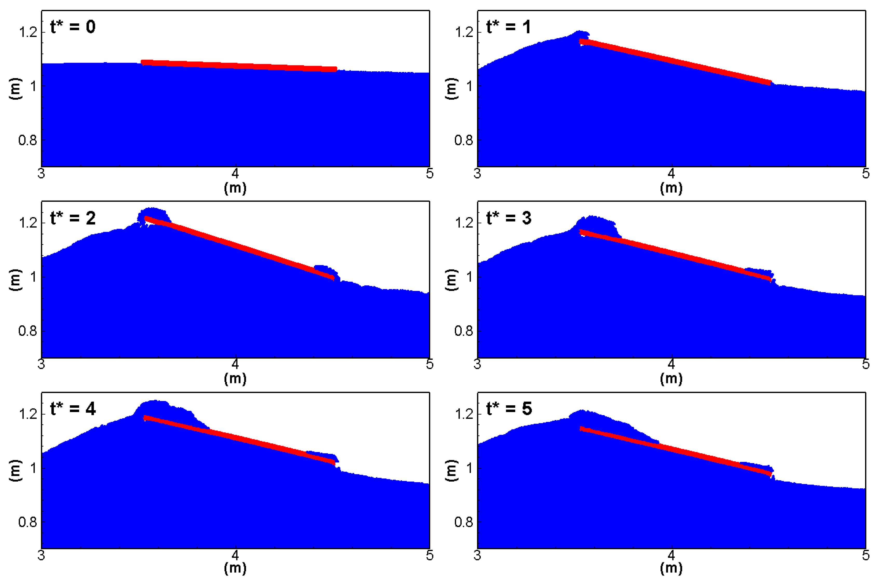
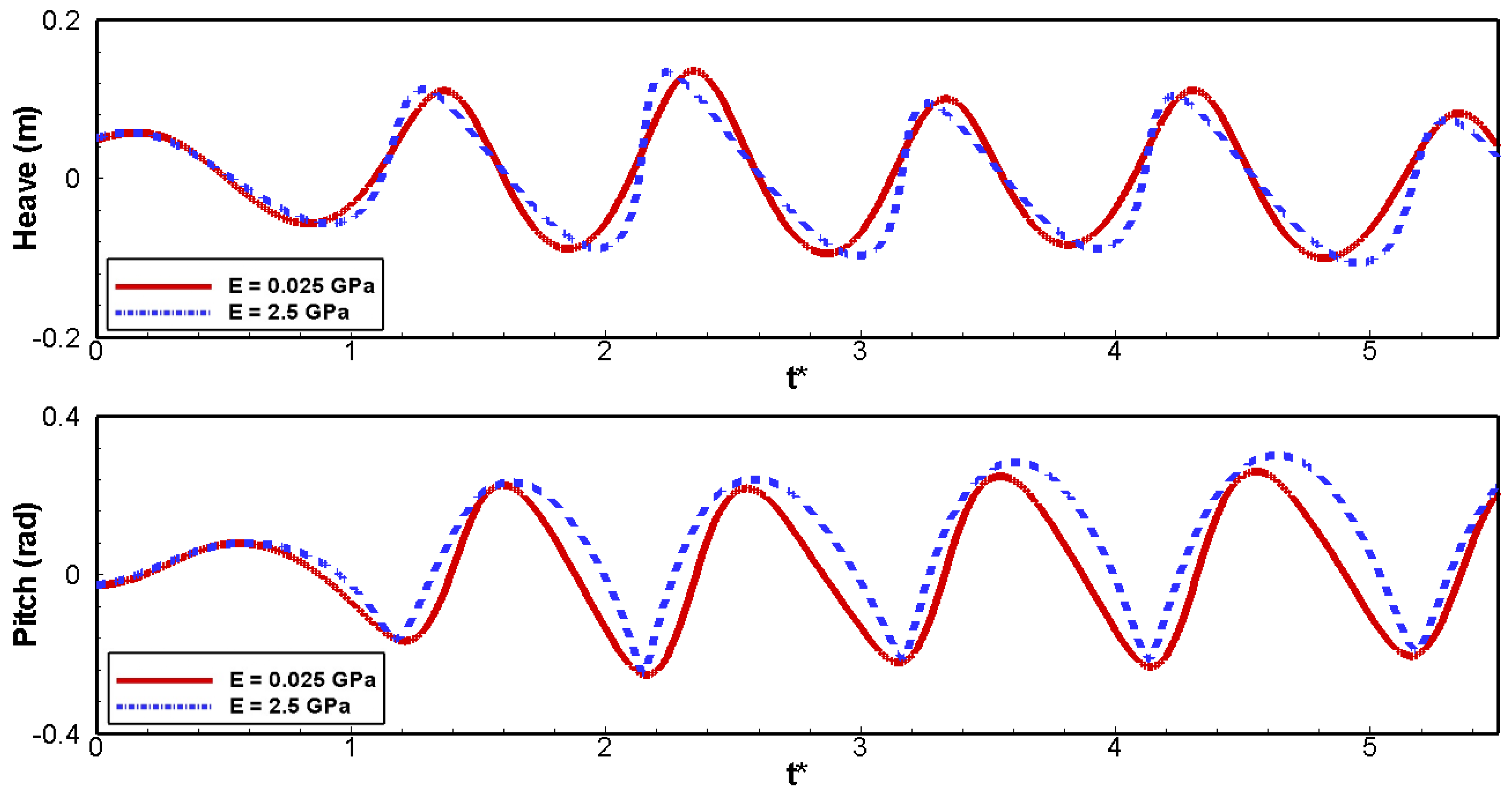
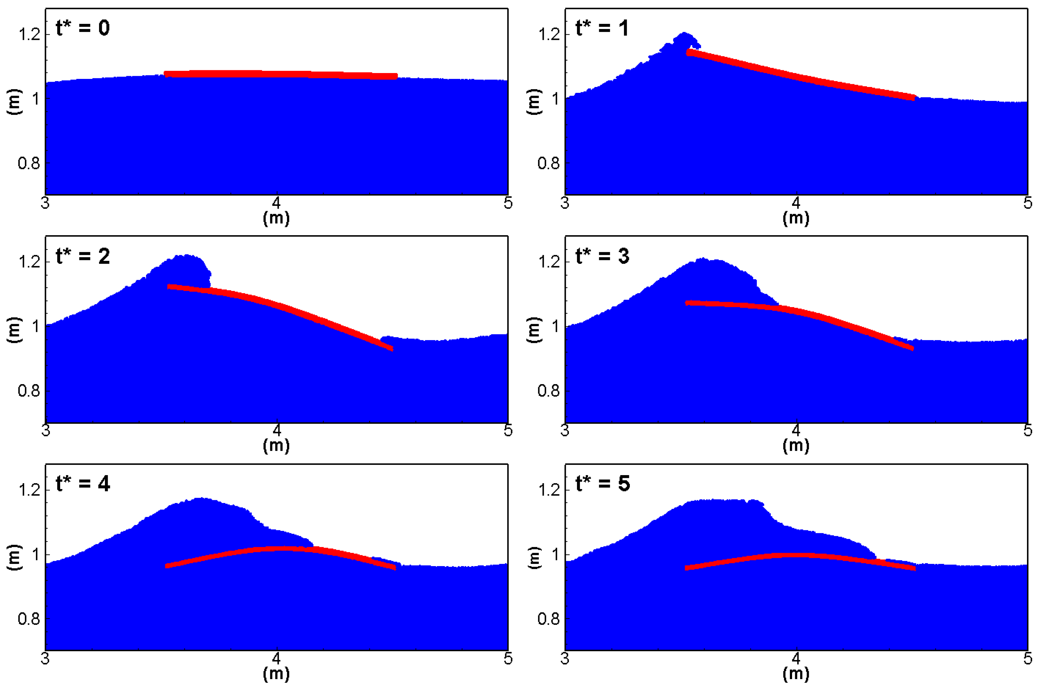
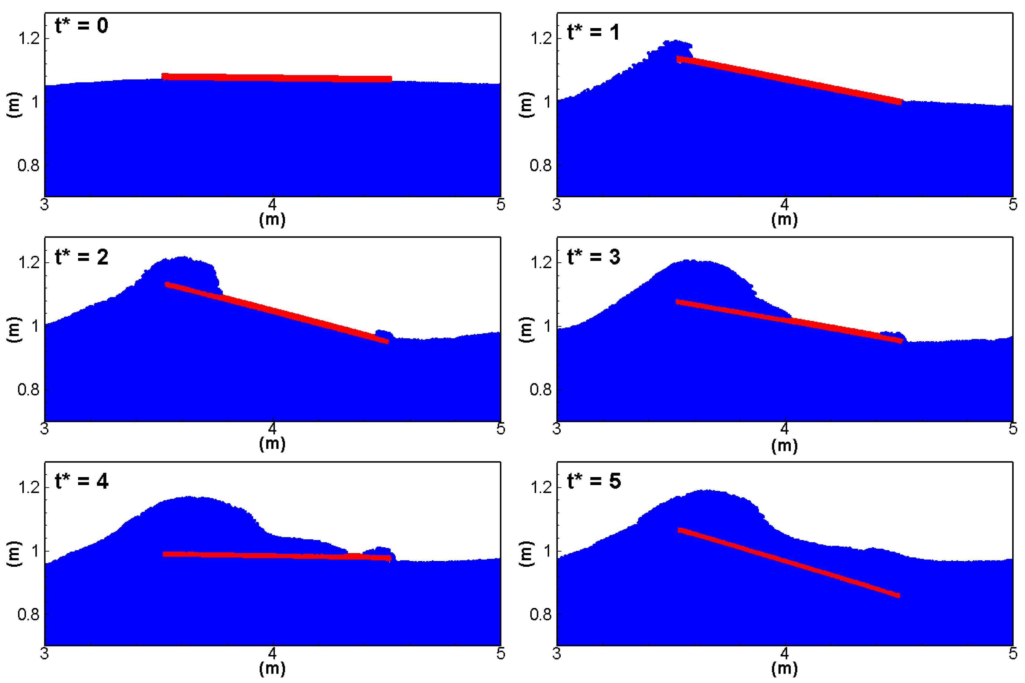
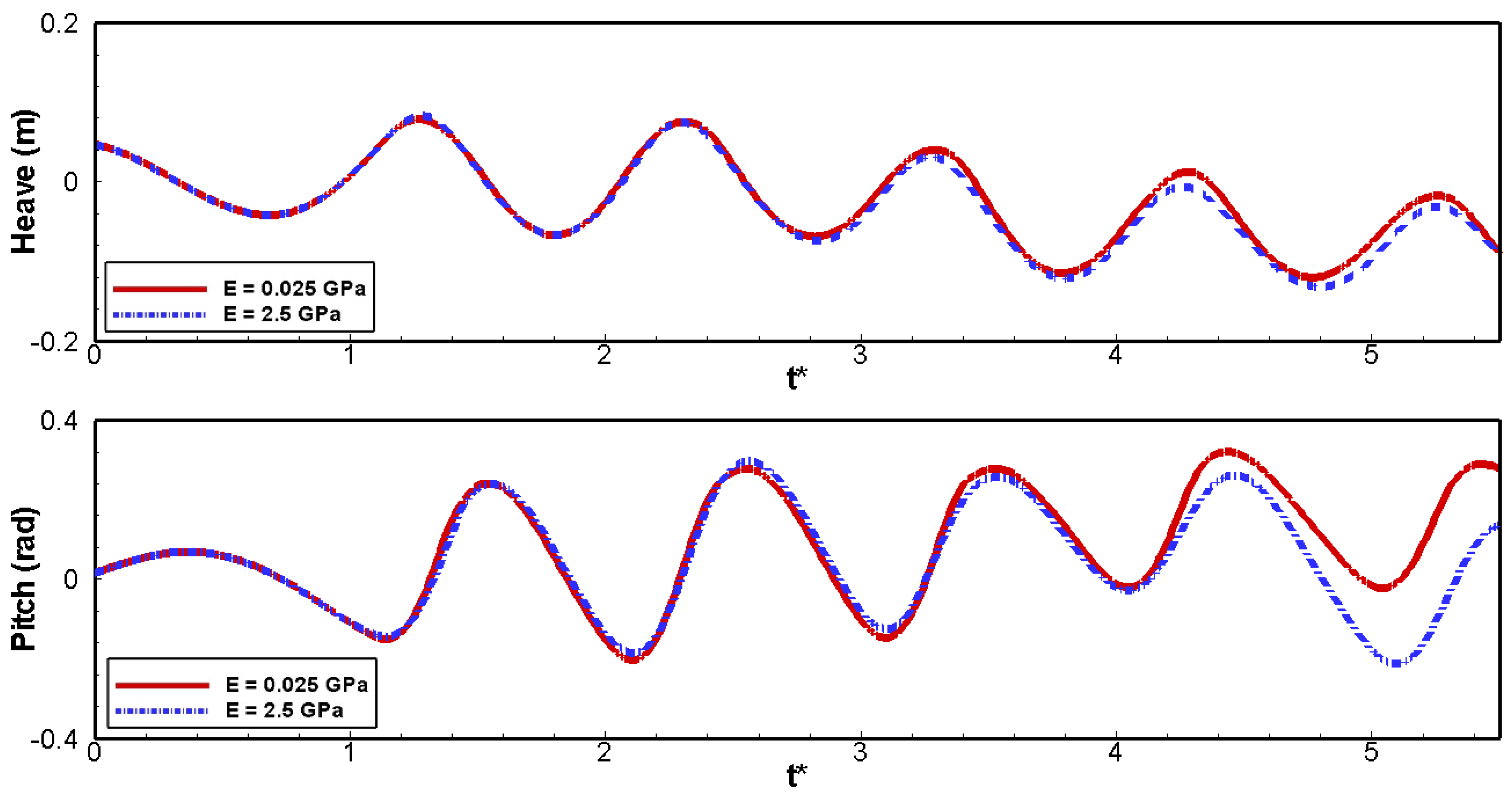
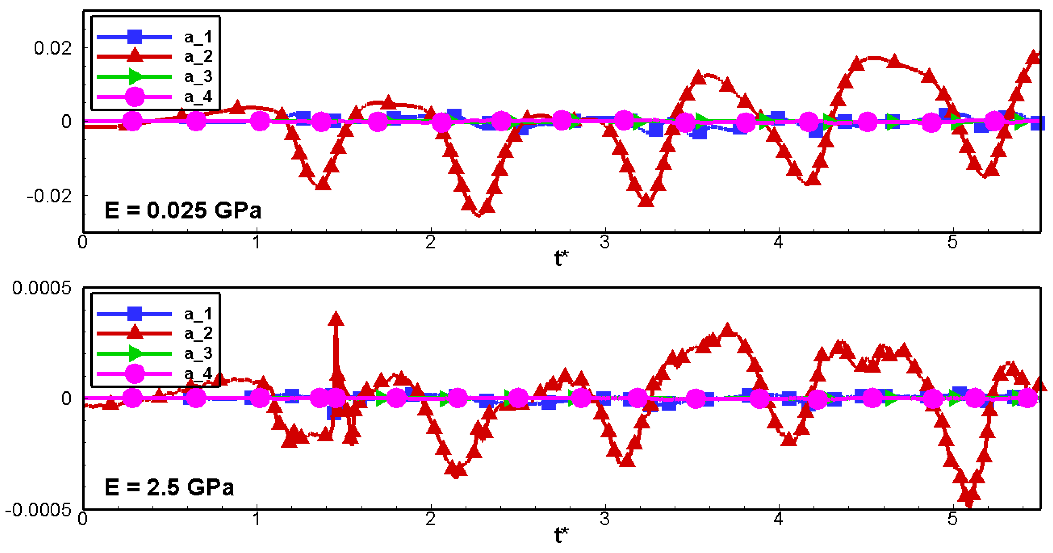
4.2. Dynamics of the Floating Plate
5. Conclusions
Author Contributions
Funding
Conflicts of Interest
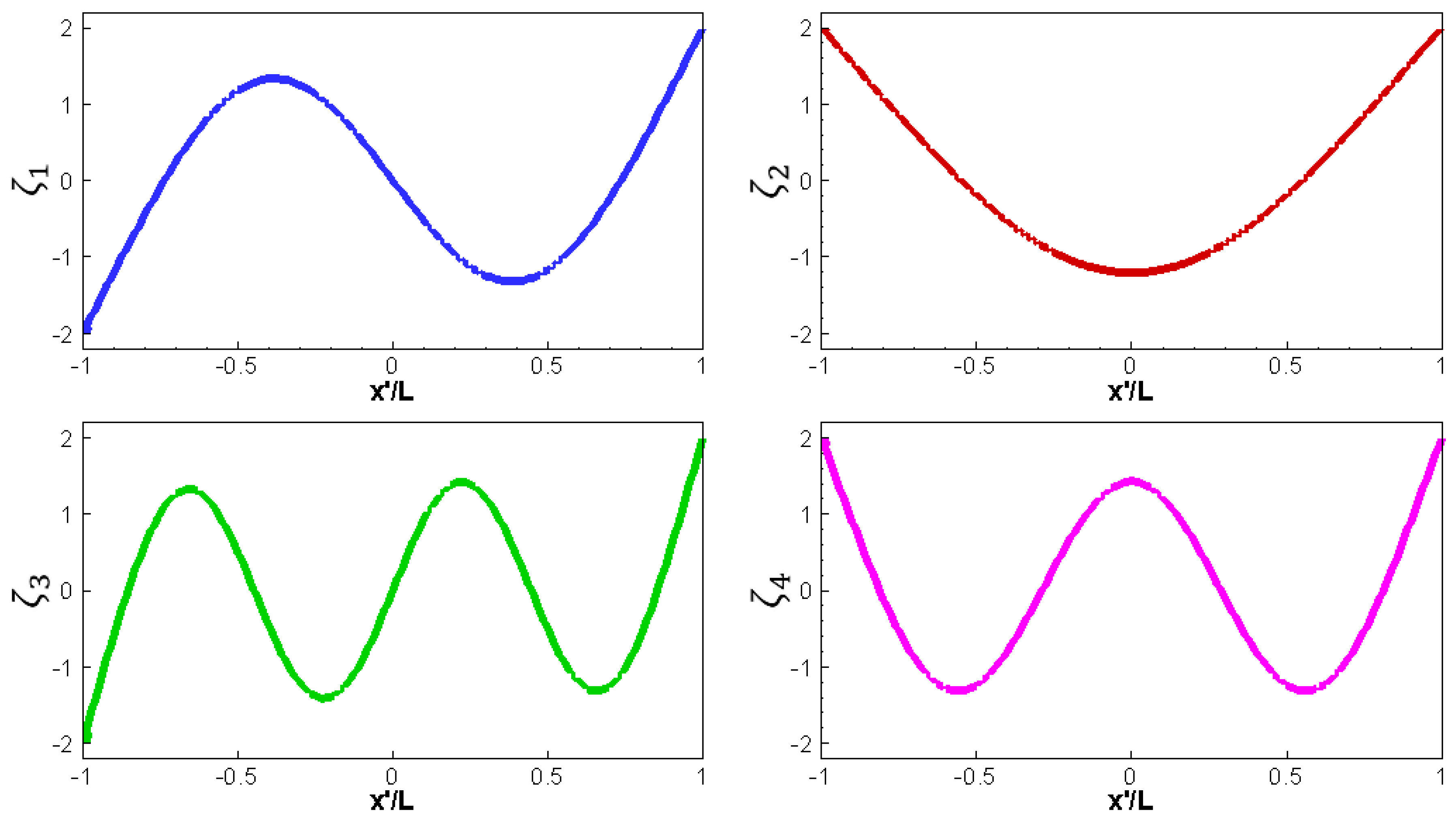
Appendix A. Vibrating Modes of a Thin Plate

| n | 1 | 2 | 3 | 4 | 5 | 6 |
|---|---|---|---|---|---|---|
| 3.926 | 2.365 | 7.068 | 5.497 | 10.210 | 8.639 |

References
- Bishop, R.E.D.; Price, W.G.; Wu, Y. A General Linear Hydroelasticity Theory of Floating Structures Moving in a Seaway. Philos. Trans. R. Soc. 1986, 316, 375–426. [Google Scholar]
- Kashiwagi, M. Research on Hydroelastic Response of VLFS: Recent Progressand Future Work. Int. J. Offshore Polar Eng. 2000, 10, 81–90. [Google Scholar]
- Squire, V.A. Synergies Between VLFS Hydroelasticity and Sea Ice Research. Int. J. Offshore Polar Eng. 2008, 18, 1–13. [Google Scholar]
- Watanabe, E.; Utsunomiya, T.; Wang, C.M. Hydroelastic analysis of pontoon-type VLFS: A literature survey. Eng. Struct. 2004, 26, 245–256. [Google Scholar] [CrossRef]
- Meylan, M.H.; Squire, V.A. The Response of Ice Floes to Ocean Waves. J. Geophys. Res. 1994, 99, 891–900. [Google Scholar] [CrossRef]
- Newman, J.N. Wave effects on deformable bodies. Appl. Ocean Res. 1994, 16, 45–101. [Google Scholar] [CrossRef]
- Meylan, M.H.; Squire, V.A. Response of a Circular Ice Floe to Ocean Waves. J. Geophys. Res. 1996, 101, 8869–8884. [Google Scholar] [CrossRef]
- Peter, M.A.; Meylan, M.H.; Chung, H. Wave scattering by a circular elastic plate in water of finite depth: A closed form solution. Int. J. Offshore Polar 2004, 14, 81–85. [Google Scholar]
- Meylan, M.H. The Wave Response of Ice Floes of Arbitrary Geometry. J. Geophys. Res. 2002, 107. [Google Scholar] [CrossRef]
- Squire, V.A. Ocean wave interactions with sea ice: A reappraisal. Annu. Rev. Fluid Mech. 2020, 52, 37–60. [Google Scholar] [CrossRef] [Green Version]
- Yago, K.; Endo, H. Model Experiment and Numerical Calculation of the Hydroelastic Behavior of Matlike VLFS. In Proceedings of the International Workshop of Very Large Floating Structures, Hayama, Japan, 25–28 November 1996; pp. 209–216. [Google Scholar]
- Kashiwagi, M. A Time-Domain Mode-Expansion Method for Calculating Transient Elastic Responses of a Pontoon-Type VLFS. J. Mar. Sci. Technol. 2000, 5, 89–100. [Google Scholar] [CrossRef]
- Kashiwagi, M. Transient responses of a VLFS during landing and take-off of an airplane. J. Mar. Sci. Technol. 2004, 9, 14–23. [Google Scholar] [CrossRef]
- Williams, T.D.; Bennetts, L.G.; Squire, V.A.; Dumont, D.; Bertino, L. Wave–ice interactions in the marginal ice zone. Part 1: Theoretical foundations. Ocean Model. 2013, 71, 81–91. [Google Scholar] [CrossRef]
- Williams, T.D.; Bennetts, L.G.; Squire, V.A.; Dumont, D.; Bertino, L. Wave–ice interactions in the marginal ice zone. Part 2: Numerical implementation and sensitivity studies along 1D transects of the ocean surface. Ocean Model. 2013, 71, 92–101. [Google Scholar] [CrossRef]
- Kohout, A.L.; Williams, M.J.; Dean, S.; Meylan, M.H. Storm-induced sea ice breakup and the implications for ice extent. Nature 2014, 509, 604–607. [Google Scholar] [CrossRef]
- Meylan, M.; Bennetts, L.; Cavaliere, C.; Alberello, A.; Toffoli, A. Experimental and theoretical models of wave-induced flexure of a sea ice floe. Phys. Fluids 2015, 27, 041704. [Google Scholar] [CrossRef]
- Bennetts, L.; Alberello, A.; Meylan, M.; Cavaliere, C.; Babanin, A.; Toffoli, A. An idealised experimental model of ocean surface wave transmission by an ice floe. Ocean Model. 2015, 96, 85–92. [Google Scholar] [CrossRef] [Green Version]
- Meylan, M.H.; Yiew, L.J.; Bennetts, L.G.; French, B.; Thomas, G.A. Surge motion of an ice floe in waves: Comparison of theoretical and experimental models. Ann. Glaciol. 2015, 56. [Google Scholar] [CrossRef] [Green Version]
- Skene, D.; Bennetts, L.; Meylan, M.; Toffoli, A. Modelling water wave overwash of a thin floating plate. J. Fluid Mech. 2015, 777, R3. [Google Scholar] [CrossRef] [Green Version]
- Toffoli, A.; Bennetts, L.G.; Meylan, M.H.; Cavaliere, C.; Alberello, A.; Elsnab, J.; Monty, J.P. Sea ice floes dissipate the energy of steep ocean waves. Geophys. Res. Lett. 2015, 42, 8547–8554. [Google Scholar] [CrossRef]
- Yiew, L.J.; Bennetts, L.G.; Meylan, M.H.; French, B.J.; Thomas, G.A. Hydrodynamic responses of a thin floating disk to regular waves. Ocean Model. 2016, 97, 52–64. [Google Scholar] [CrossRef] [Green Version]
- Dolatshah, A.; Nelli, F.; Bennetts, L.G.; Alberello, A.; Meylan, M.; Monty, J.; Toffoli, A. Hydroelastic interactions between water waves and floating freshwater ice. Phys. Fluids 2018, 30, 091702. [Google Scholar] [CrossRef] [Green Version]
- Zhang, X.; Draper, S.; Wolgamot, H.; Zhao, W.; Cheng, L. Eliciting features of 2D greenwater overtopping of a fixed box using modified dam break models. Appl. Ocean Res. 2019, 84, 74–91. [Google Scholar] [CrossRef]
- Montiel, F.; Bennetts, L.G.; Squire, V.A.; Bonnefoy, F.; Ferrant, P. Hydroelastic response of floating elastic discs to regular waves. Part 1. Wave basin experiments. J. Fluid Mech. 2013, 723, 604–628. [Google Scholar] [CrossRef] [Green Version]
- Skene, D.; Bennetts, L.; Wright, M.; Meylan, M.; Maki, K. Water wave overwash of a step. J. Fluid Mech 2018, 839, 293–312. [Google Scholar] [CrossRef]
- Huang, L.; Ren, K.; Li, M.; Tuković, Ž.; Cardiff, P.; Thomas, G. Fluid-structure interaction of a large ice sheet in waves. Ocean Eng. 2019, 182, 102–111. [Google Scholar] [CrossRef] [Green Version]
- Nelli, F.; Bennetts, L.G.; Skene, D.M.; Toffoli, A. Water wave transmission and energy dissipation by a floating plate in the presence of overwash. J. Fluid Mech. 2020, 889. [Google Scholar] [CrossRef]
- Capone, T.; Panizzo, A.; Monaghan, J.J. SPH modelling of water waves generated bysubmarine landslides. J. Hydraul. Res. 2010, 48, 80–84. [Google Scholar] [CrossRef]
- Bian, X.; Ellero, M. A splitting integration scheme for the SPH simulation of concentrated particle suspensions. Comput. Phys. Commun. 2014, 185, 53–62. [Google Scholar] [CrossRef]
- Tran-Duc, T.; Ho, T.; Thamwattana, N. A Smoothed Particle Hydrodynamics Study on Effect of Coarse Aggregate on Self-Compacting Concrete Flows. Int. J. Mech. Sci. 2021, 190, 106046. [Google Scholar] [CrossRef]
- Dalrymple, R.A.; Rogers, B. Numerical modeling of water waves with the SPH method. Coast. Eng. 2006, 53, 141–147. [Google Scholar] [CrossRef]
- Crespo, A.J.C.; Altomare, C.; Domínguez, J.M.; González-Cao, J.; Gómez-Gesteira, M. Towards simulating floating offshore oscillating water column converters with Smoothed Particle Hydrodynamics. Coast. Eng. 2017, 126, 11–26. [Google Scholar] [CrossRef]
- Wen, H.; Ren, B.; Dong, P.; Wang, Y. A SPH numerical wave basin for modeling wave-structure interactions. Appl. Ocean Res. 2016, 59, 366–377. [Google Scholar] [CrossRef] [Green Version]
- Zhang, N.; Zheng, X.; Ma, Q. Study on wave-induced kinematic responses and flexures of ice floe by Smoothed Particle Hydrodynamics. Comput. Fluids 2019, 189, 46–59. [Google Scholar] [CrossRef]
- McGovern, D.J.; Bai, W. Experimental Study on Kinematics of Sea Ice Floes in Regular Waves. Cold Reg. Sci. Technol. 2014, 103, 15–30. [Google Scholar] [CrossRef]
- Murray, J.J.; Guy, G.B.; Muggeridge, D.B. Response of Modelled Ice Masses to Regular Waves and Regular Wave Groups. In Proceedings of the OCEANS ’83, San Francisco, CA, USA, 29 August–1 September 1983; pp. 1048–1052. [Google Scholar]
- Lever, J.H.; Attwood, D.; Sen, D. Factors Affecting the Prediction of Wave-Induced Iceberg Motion. Cold Reg. Sci. Technol. 1988, 15, 177–190. [Google Scholar] [CrossRef]
- Mei, C.C. The Applied Dynamics of Ocean Surface Waves; World Scientific: Singapore, 1989. [Google Scholar]
- Ni, X.; Feng, W.; Huang, S.; Zhang, Y.; Feng, X. A SPH numerical wave flume with non-reflective open boundary conditions. Ocean Eng. 2018, 163, 483–501. [Google Scholar] [CrossRef]
- Wen, H.; Ren, B. A non-reflective spectral wave maker for SPH modeling of nonlinear wave motion. Wave Motion 2018, 79, 112–128. [Google Scholar] [CrossRef]
- Cabezón, R.M.; García-Senz, D.; Relaño, A. A One-Parameter Family of Interpolating Kernels for Smoothed Particle Hydrodynamics Studies. J. Comput. Phys. 2008, 227, 8523–8540. [Google Scholar] [CrossRef] [Green Version]
- Cummins, S.J.; Rudman, M. An SPH Projection Method. J. Comp. Phys. 1999, 152, 584–607. [Google Scholar] [CrossRef]
- Nomeritae, N.; Daly, E.; Grimaldi, S.; Bui, H.H. Explicit Incompressible SPH Algorithm for Free-Surface Flow Modelling: A Comparison with Weakly Compressible Schemes. Adv. Water Res. 2016, 97, 156–167. [Google Scholar] [CrossRef]
- Xu, R.; Stansby, P.; Laurence, D. Accuracy and Stability in Incompressible SPH (ISPH) Based on the Projection Method and a New Approach. J. Comp. Phys. 2009, 228, 6703–6725. [Google Scholar] [CrossRef]
- Shao, S.; Lo, E. Incompressible SPH method for simulating Newtonian and non-Newtonian flows with a free surface. Adv. Water Res. 2003, 203, 787–800. [Google Scholar] [CrossRef]
- Akbari, H. An Improved Particle Shifting Technique for Incompressible Smoothed Particle Hydrodynamics Methods. Int. J. Numer. Meth. Fluids 2019, 90, 603–631. [Google Scholar] [CrossRef]
- Lee, E.S.; Moulinec, C.; Xu, R.; Violeau, D.; Laurence, D.; Stansby, P. Comparisons of Weakly Compressible and Truly Incompressible Algorithms for the SPH Mesh Free Particle Method. J. Comput. Phys. 2008, 227, 8417–8436. [Google Scholar] [CrossRef]
- Altomare, C.; Domínguez, J.M.; Crespo, A.; Gonzáles-Cao, J.; Suzuki, T.; Gómez-Gesteira, M.; Troch, P. Long-Crested Wave Generation and Absorption for SPH-Based DualSPHysics Model. Coast. Eng. 2017, 127, 37–54. [Google Scholar] [CrossRef]
- Trimulyono, A.; Hashimoto, H.; Matsuda, A. Experimental Validation of Single- and Two-Phase Smoothed Particle Hydrodynamics on Sloshing in a Prismatic Tank. J. Mar. Sci. Eng. 2019, 7, 247. [Google Scholar] [CrossRef] [Green Version]
- Arunachalam, V.M.; Murray, J.J.; Muggeridge, D.B. Short Term Motion Analysis of Icebergs in Linear Waves. Cold Reg. Sci. Technol. 1987, 13, 247–258. [Google Scholar] [CrossRef]
- Huang, L.; Bennetts, L.; Cardiff, P.; Jasak, H.; Tukovic, Z.; Thomas, G. The implication of elastic deformation in wave-ice interaction. In Proceedings of the 15th OpenFOAM Workshop, Arlington, VA, USA, 22–25 June 2020. [Google Scholar]
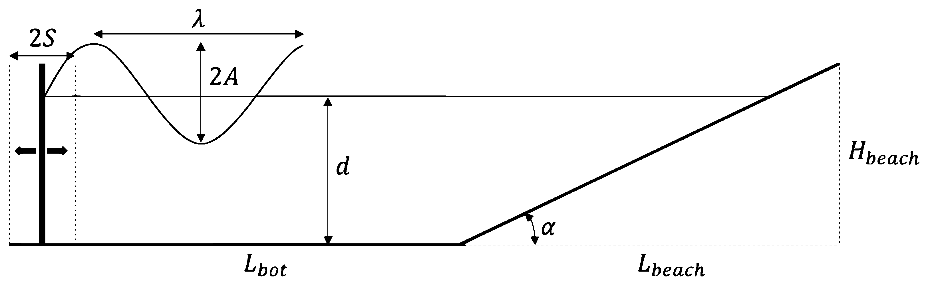


| Parameters | Current Work | Zhang et al. [35] |
|---|---|---|
| Wave | ||
| Period T (s) | 1.2, 1.5 | 0.6, 1.2 |
| Amplitude A (m) | 0.187, 0.159 | 0.0064, 0.016, 0.024 |
| Length (m) | 2.35, 3.38 | 1.0 |
| Steepness | 0.295, 0.5 | 0.04, 0.1, 0.15 |
| Floating plate | ||
| Young modulus E (GPa) | 0.025, 2.5 | 0.5 |
| Thickness (m) | 0.02 | 0.01 |
| Length (m) | 1.0 | 1.0 |
| Density (kg/m) | 500.0 | 500.0 |
| Ratio of wavelength to the plate length | 2.35, 3.38 | 1 |
Publisher’s Note: MDPI stays neutral with regard to jurisdictional claims in published maps and institutional affiliations. |
© 2020 by the authors. Licensee MDPI, Basel, Switzerland. This article is an open access article distributed under the terms and conditions of the Creative Commons Attribution (CC BY) license (http://creativecommons.org/licenses/by/4.0/).
Share and Cite
Tran-Duc, T.; Meylan, M.H.; Thamwattana, N.; Lamichhane, B.P. Wave Interaction and Overwash with a Flexible Plate by Smoothed Particle Hydrodynamics. Water 2020, 12, 3354. https://doi.org/10.3390/w12123354
Tran-Duc T, Meylan MH, Thamwattana N, Lamichhane BP. Wave Interaction and Overwash with a Flexible Plate by Smoothed Particle Hydrodynamics. Water. 2020; 12(12):3354. https://doi.org/10.3390/w12123354
Chicago/Turabian StyleTran-Duc, Thien, Michael H. Meylan, Ngamta Thamwattana, and Bishnu P. Lamichhane. 2020. "Wave Interaction and Overwash with a Flexible Plate by Smoothed Particle Hydrodynamics" Water 12, no. 12: 3354. https://doi.org/10.3390/w12123354
APA StyleTran-Duc, T., Meylan, M. H., Thamwattana, N., & Lamichhane, B. P. (2020). Wave Interaction and Overwash with a Flexible Plate by Smoothed Particle Hydrodynamics. Water, 12(12), 3354. https://doi.org/10.3390/w12123354