This chapter presents the ANEMI model, which is currently in version 3 [
19,
20], built upon the first two iterations of ANEMI [
21,
22]. The model shares the same system dynamics simulation paradigm that was used in the previous iterations of ANEMI, in that feedbacks and delays are used to drive system behavior. ANEMI3 is a type of integrated assessment model that describes the state of and interactions between model sub-systems that compose the Earth system. The main sub-systems or ‘sectors’ used are that of the climate system, carbon, nutrient and hydrologic cycles, population dynamics, land use, food production, sea level rise, energy production, global economy, persistent pollution, water demand and water supply development.
The boundary of the model is defined by the problem that is being explored. In this case, we are modelling the role of water resources in various aspects of global change. Therefore, the spatial scale of the model is mainly one that is global. In some sectors, the stocks are disaggregated to capture material flows on a sub-global scale but not at a level that is location specific. This spatial scale limits the level of detail that can be used to describe the flows that act to change the model stocks, however it allows us to effectively analyze feedbacks between water resources and other model sectors on a global scale.
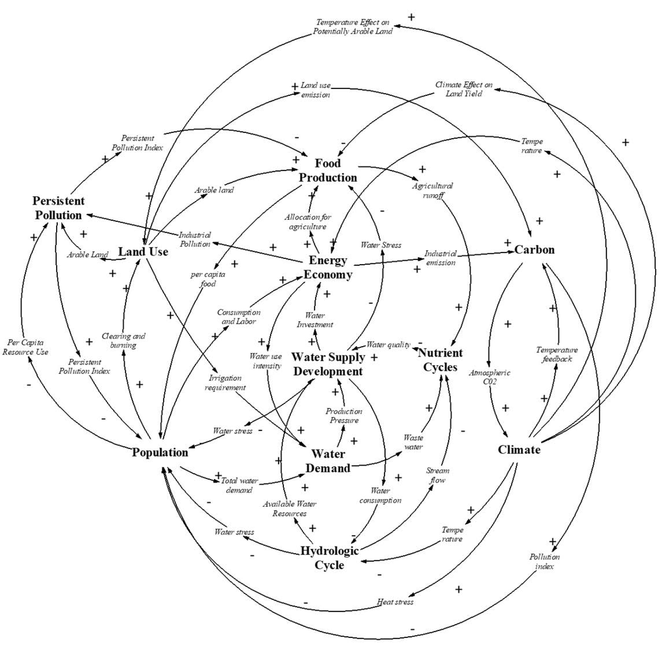
The highly endogenous structure and coupling of sub-systems in the ANEMI3 model are part of its novelty in the realm of integrated assessment modelling. Because of this, feedback processes are responsible for the behavior that is exhibited in model runs. The model sectors that comprise the ANEMI3 model are that of the climate system, carbon, nutrient and hydrologic cycles, population dynamics, land use, food production, sea level rise, energy production, global economy, persistent pollution, water demand and water supply development as shown in
Figure 1. The model includes over 2000 variables and 700 equations. Presentation in
Figure 1 is focused on illustrating the high-level model sectoral structure and relationships. Feedback loops between sectors or intersectoral feedback loops are responsible for global change in this Earth system. Intersectoral feedbacks in the ANEMI3 model allow for the representation of various aspects of global change. In the
Figure 1 diagram alone there is a total of 89 possible intersectoral feedback loops. The size of the feedback loops range from 2 to 9 sectors included out of the 10 that are shown. An example is that of a growing global economy, which drives energy production and industrial growth, thereby resulting in more greenhouse gas emissions and climate change. This in turn results in negative feedbacks on economic growth through climate damages, which can represent economic damages because of land and structures lost to coastal flooding, for example. Creating a causal loop diagram from these connections between model sectors allows us to view the feedbacks that are created by combining model sectors in this way.
The main difference between ANEMI1, ANEMI2 and ANEMI3 is addition of intersectoral feedback loops used to (a) analyze water supply development within the Earth system, (b) include of water quality degradation and its impact on the development of surface water supplies and (c) assess of global scale feedback related to water supply development. These main modifications are introduced to represent the dynamics of global change at the global scale with an emphasis on the development of water supplies.
2.1. Integrated Assessment of Global Water Resources
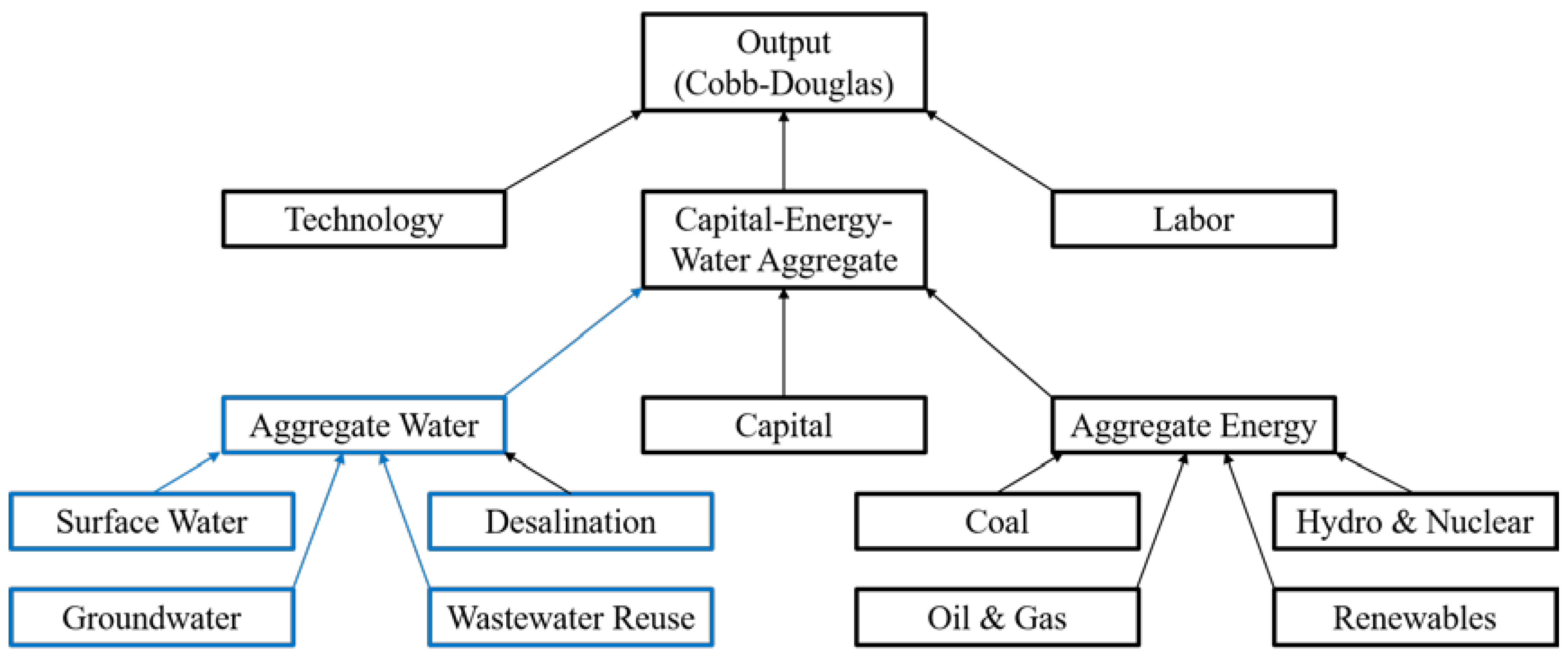
The new water supply sector in ANEMI3 was developed by incorporating water supply as a new production sector within the newly added energy-economy sector [
19,
20,
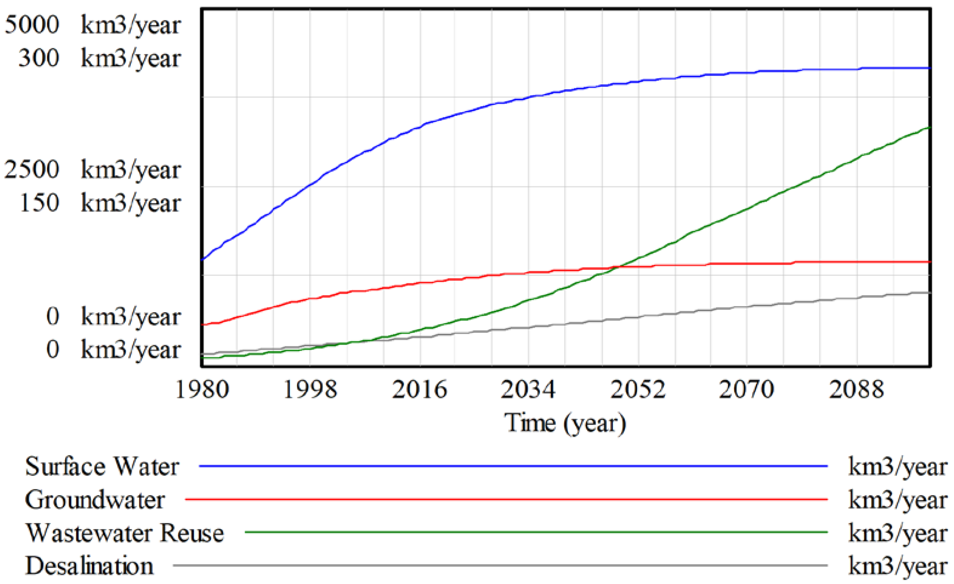
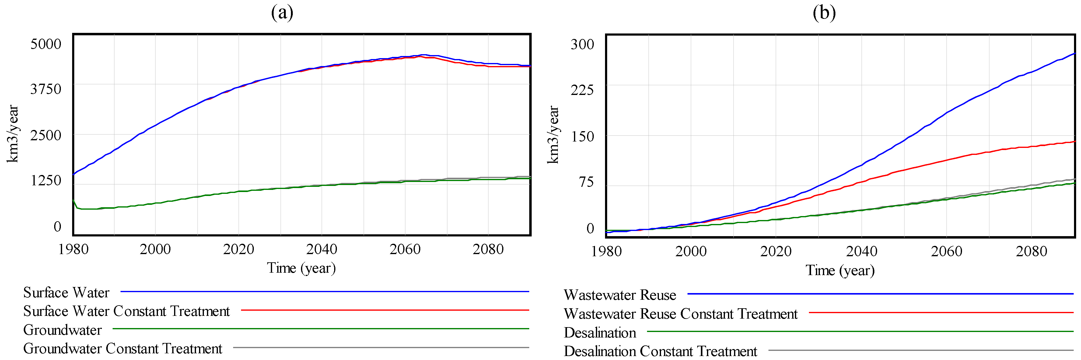
23]. This has been achieved by adding capital stocks to produce water supply in the form of surface, ground, wastewater reclamation and desalination water sources.
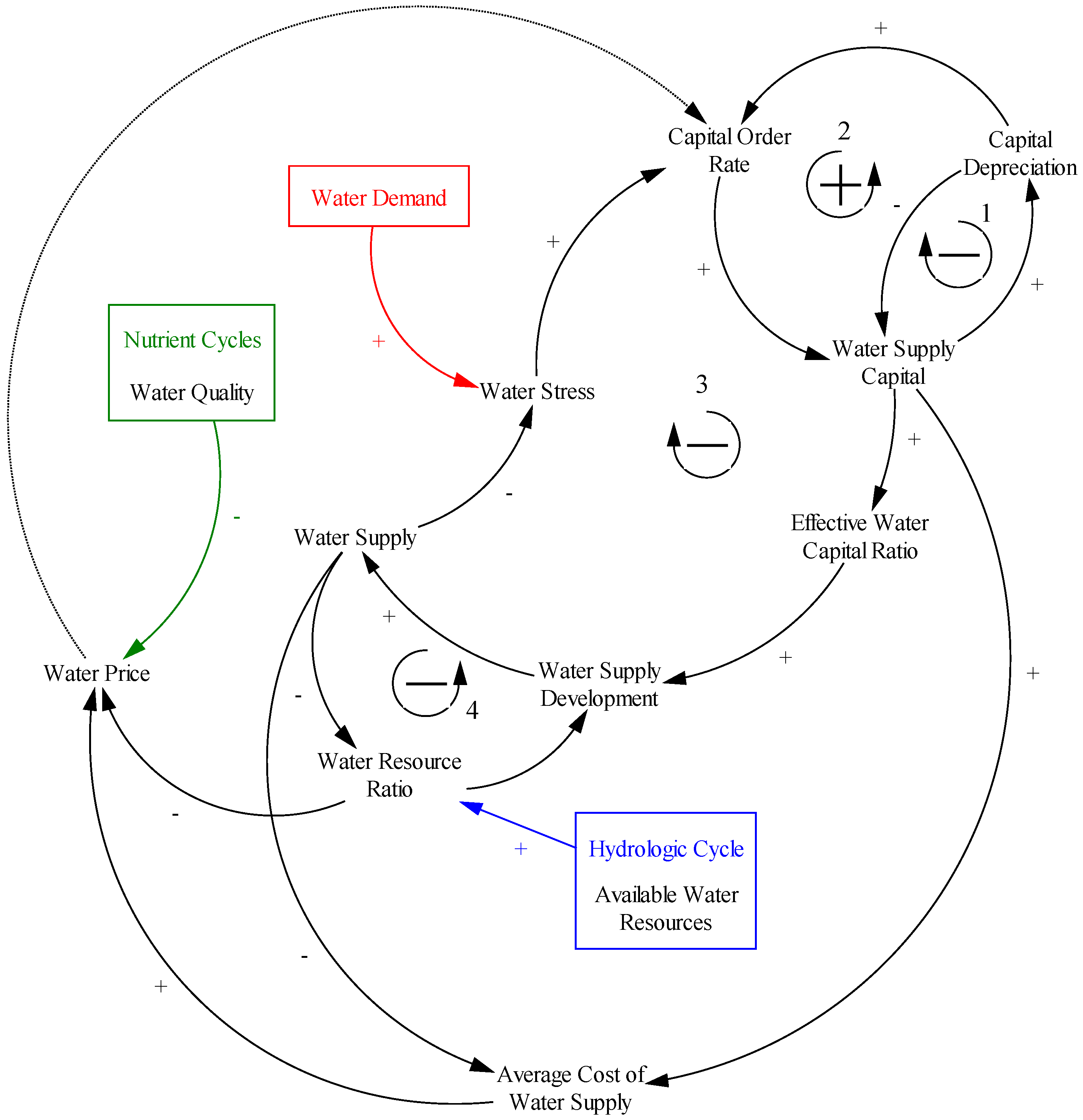
As available water resources become depleted, the water supply is reduced for the same input intensity. This means that more effort is required to produce the same rate of water supply, which also makes a given type of water supply that is depleted more expensive. For example, when the groundwater elevation decreases from over abstraction, more pumping energy is required to extract the same amount of water resource. The effect of saturation is also included in this relationship, assuming the best or most cost-effective sites are used first for water supply infrastructures. An example of which could include the construction of additional reservoirs, source water intakes, of groundwater wells in areas that are less suitable or cost effective than those that were previously constructed.
The dotted causal link from water price to the capital order rate in
Figure 2 indicates a connection that is neither positive nor negative. Instead, this link is used to determine the amount of investment that is made in the capital stocks of the different supply types (surface, ground, wastewater reclamation and desalination water sources). Inputs from the nutrient cycle, hydrologic cycle and water demand sectors are used to define the water price, water stress and water resource ratio variables respectively in the water supply development sector.
2.2. Mathematical Formulation of Water Supply Development Sector
Water resources,
are used in the production of water supplies, where the subscript
, denotes the type of water supplies for which the water resources are being used.
where
= Surface water resources
;
= Groundwater resources
;
= Wastewater resources
;
= Desalination water resources;
= Stable and reusable runoff fraction;
TRF = Total renewable flow
;
WPF = Wastewater pollution factor;
= Percolation to groundwater
;
= Groundwater discharge
;
TDW = Treated domestic wastewater
;
TIW = Treated industrial wastewater
;
URW = Untreated Returnable Waters
.
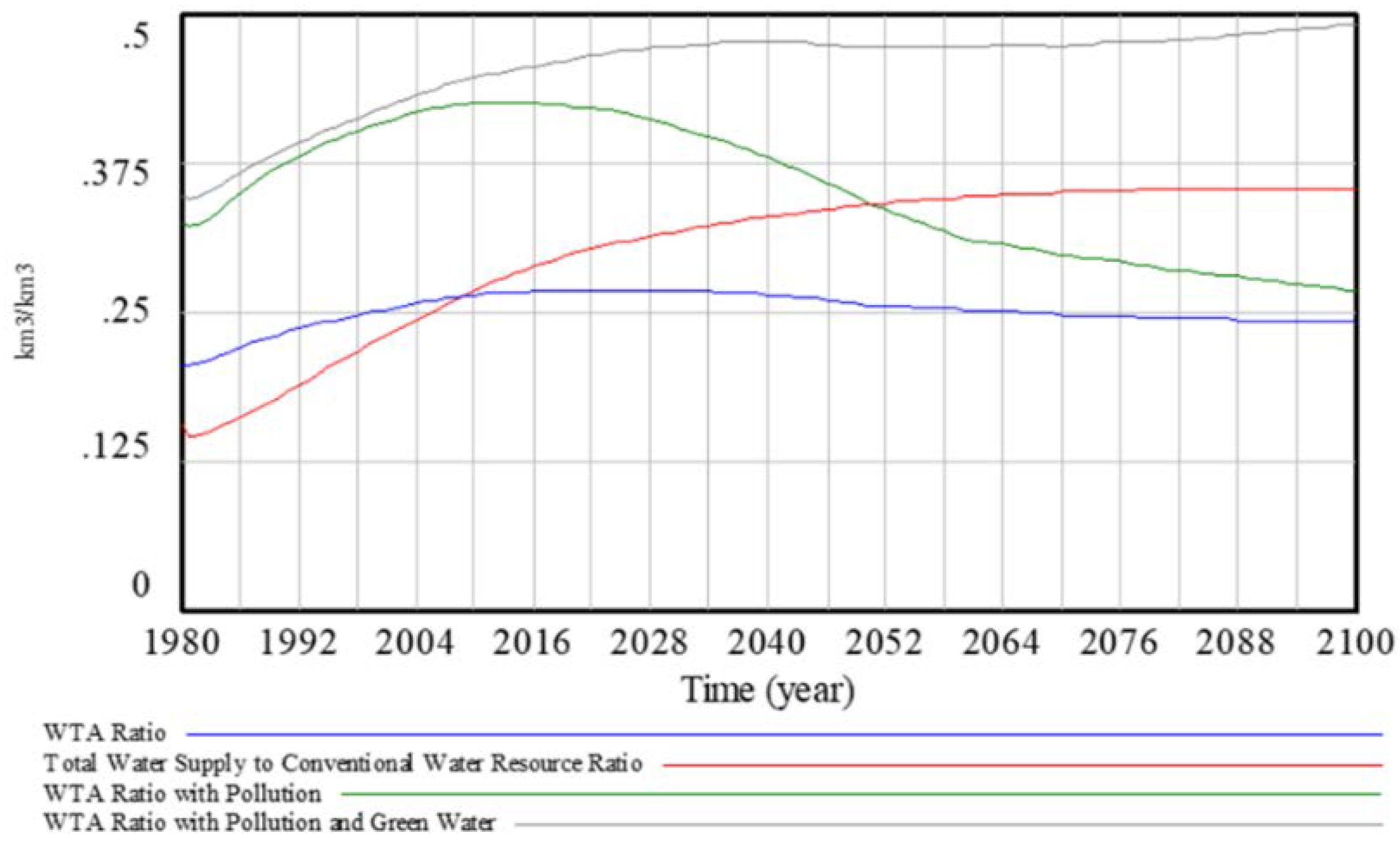
The amount of water resources available for the development of water supplies is dependent on the hydrologic cycle, water demand and water quality sectors of the model. In the case of surface water, the stable and reusable portion of runoff is taken from the total renewable streamflow and is adjusted for untreated wastewater discharge. The adjustment for wastewater discharge is based on [
24] which estimates that for every cubic meter of contaminated wastewater discharged into water bodies and streams, makes unsuitable 8–10 cubic meters of fresh water. The difference in groundwater percolation and discharge is used for the consideration of groundwater resources as this refers to renewable groundwater. Only renewable groundwater resources are considered for the global scale. The inclusion of non-renewable or fossil groundwater resources should be considered at the regional scale. For the potential reuse of wastewater, industrial and domestic wastewaters are considered. Although the reuse of wastewater is highly dependent on the type of wastewater and the use for which it is being treated, it is considered here as a supplementary type of water supply in the case of groundwater and surface water depletion. Water resources used for desalination are considered primarily from the ocean stock in the hydrologic cycle. This results in a virtually limitless supply; however, it is very energy intensive resulting in a high effective input intensity thereby limiting production.
The concept of resource depletion in energy production is also applicable to water supply development. For example, in the case of surface water and groundwater resources, depleted water resources will mean less suitable locations for water extraction and treatment plants. This might mean that source waters could be further from where the water is being used, thus increasing distribution costs. Pumping costs could also be increased by using deeper aquifers or surface water supplies that have a greater difference in elevation from their point of use. Water resource depletion factors into the water supply development process in much the same way as energy production, however there is one key difference. The depletion effect for energy production is based on the ratio of current energy resources remaining to the initial amount. In contrast, water resources are renewable to varying degrees. Therefore, simply taking the ratio of the available water resources to the initial water resources is insufficient. Here, the ratio of available water resources to the current production level is used. In order to accomplish this structure, water production was changed to a stock variable to avoid creating an indeterminate system (introduction of a new negative feedback by making water production a function of itself).
where
= Water supply from water resource
i ;
= Initial water production
;
= Available water resource remaining
;
= Effective water input intensity;
= Water resource share;
= Resource substitution coefficient.
In the case of surface water, the available water resources are a rate (runoff minus water quality depletion effects) rather than a stock that can be depleted over time. If production equals this rate, then there is no more surface water that can be utilized at this time step. For wastewater reuse if the rate of reuse is equal to that of the amount of treated wastewater, then no more wastewater can be reused unless wastewater treatment percentage increases.
In the energy capital sub-system of the energy-economy sector, the desired energy capital for each source is determined by the perceived return on investment and the production pressure defined as the ratio of the energy order rate or demand to energy production for each source [
19,
20]. In the case of water supply, the term for perceived return on investment is removed, thereby making the primary drive for new water supply capital based on production pressure, which resembles the definition of water stress (withdrawal or demand to availability ratio). This value is multiplied by the current water capital stocks to obtain the desired water capital stocks,
where
. = Desired water capital for water source
i ;
= Demand for water supply
i ;
= Water supply from water source
i .
Where
denotes the type of water supply for which desired water capital is being determined. In order to obtain the demand for water supply from each source, Wood’s algorithm [
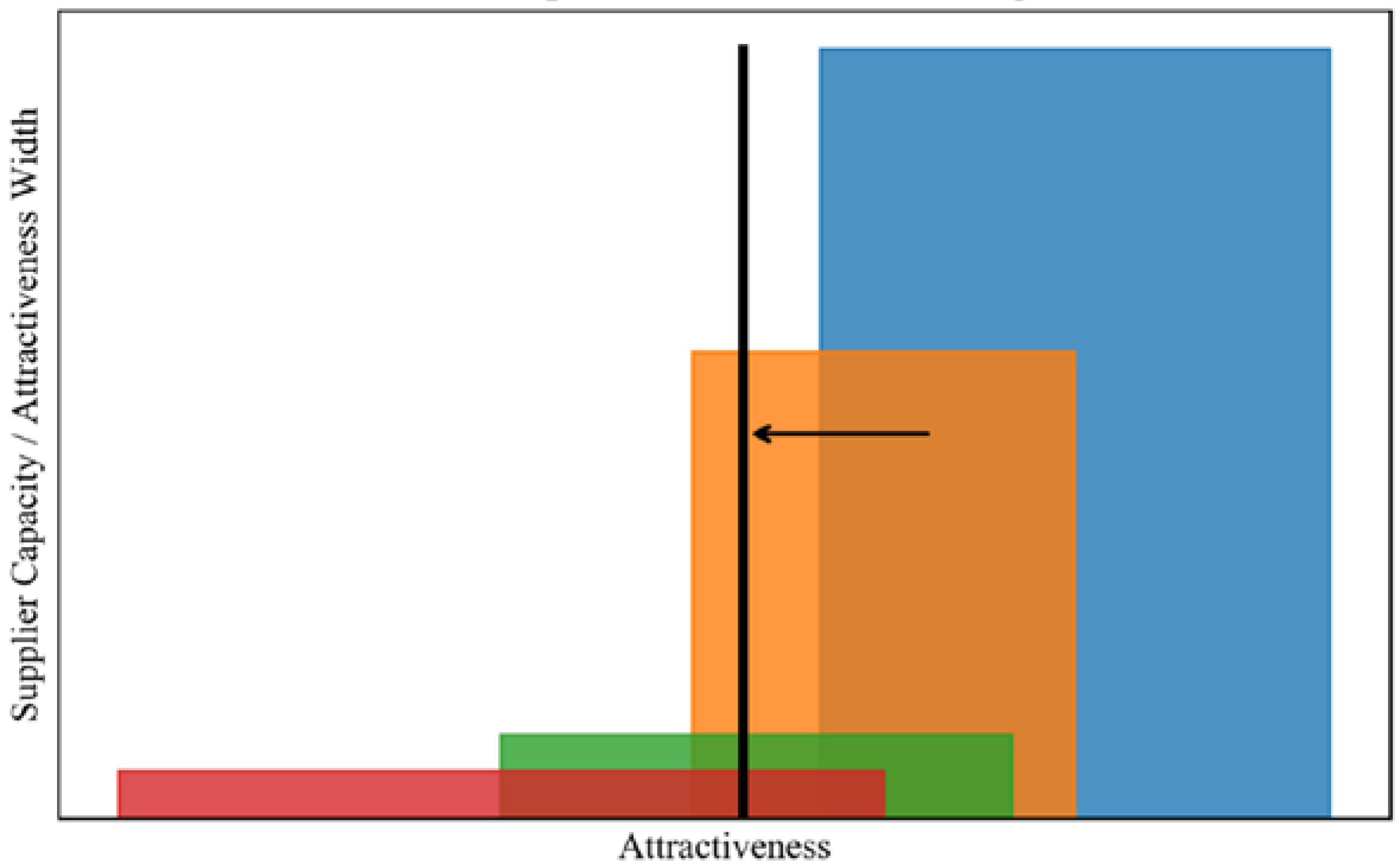
21] is used to allocate the total water demand (sum of domestic, industrial and agricultural water demand) to each supplier. The geometric illustration of Wood’s algorithm is shown in
Figure 3, where each rectangle represents a different supplier (blue-surface, orange-ground, green-wastewater reclamation and red-desalination water supplies). The area of each rectangle represents the capacity for a given supplier to fulfil the demand for a product, while the position and width of each rectangle is based on the “attractiveness” value and “width” parameters respectively. Here, the inverse water supply price is used to represent the attractiveness value and the area of each rectangle would be the water supply capacity for a given supply type. The total water demand is allocated to each supplier by the black line in
Figure 3 which moves from right to left until the area to the right of the line fulfils the demand. The area of each rectangle that lies on the right of the black line represents the level of demand satisfied by each supplier, therefore a water supply type with a high price would be placed farther to the left on the attractiveness scale and would receive less of the total water demand.
The inverse water supply price was chosen as the main driver for changes in supplier attractiveness as this will vary with technological improvements, depletion, saturation and water quality in the case of surface water supply. This formulation encapsulates the effects of global changes in technology, water resource availability and water quality on the allocation of capital investments in different types of water supply. The width factor determines how this allocation is distributed to suppliers which are not necessarily the cheapest option. For example, on the global scale, although the use of surface water supplies is likely the most cost-effective option in many regions, groundwater, water reuse and desalination supplies are all being used simultaneously.
The concept of endogenous technological change applied to energy production [
19,
20] has analogies to water supply development. In the case of surface water and groundwater supplies, it is assumed that pumping, distribution and treatment technologies will remain largely the same but will show some improvement over time. However, alternative water supplies such as wastewater reuse and desalination are likely to see vast improvements in the near future. Factoring technological change into the water supply development process is what will help make alternative water supplies more feasible in the future, along with depletion and saturation of conventional water supplies.
A unique attribute of water resources when considering water supply development is water quality. Degraded water quality can impact the functioning of water treatment facilities as well as maintenance costs and the necessary configuration of unit processes [
22]. This may also influence the ability to secure adequate source waters for extraction of water resources in the future as a result of pollution and climate change. This could negatively impact production of conventional water supplies by increasing the cost of implementing new capital as well as variable inputs needed for treatment and distribution including energy, chemicals and labor.
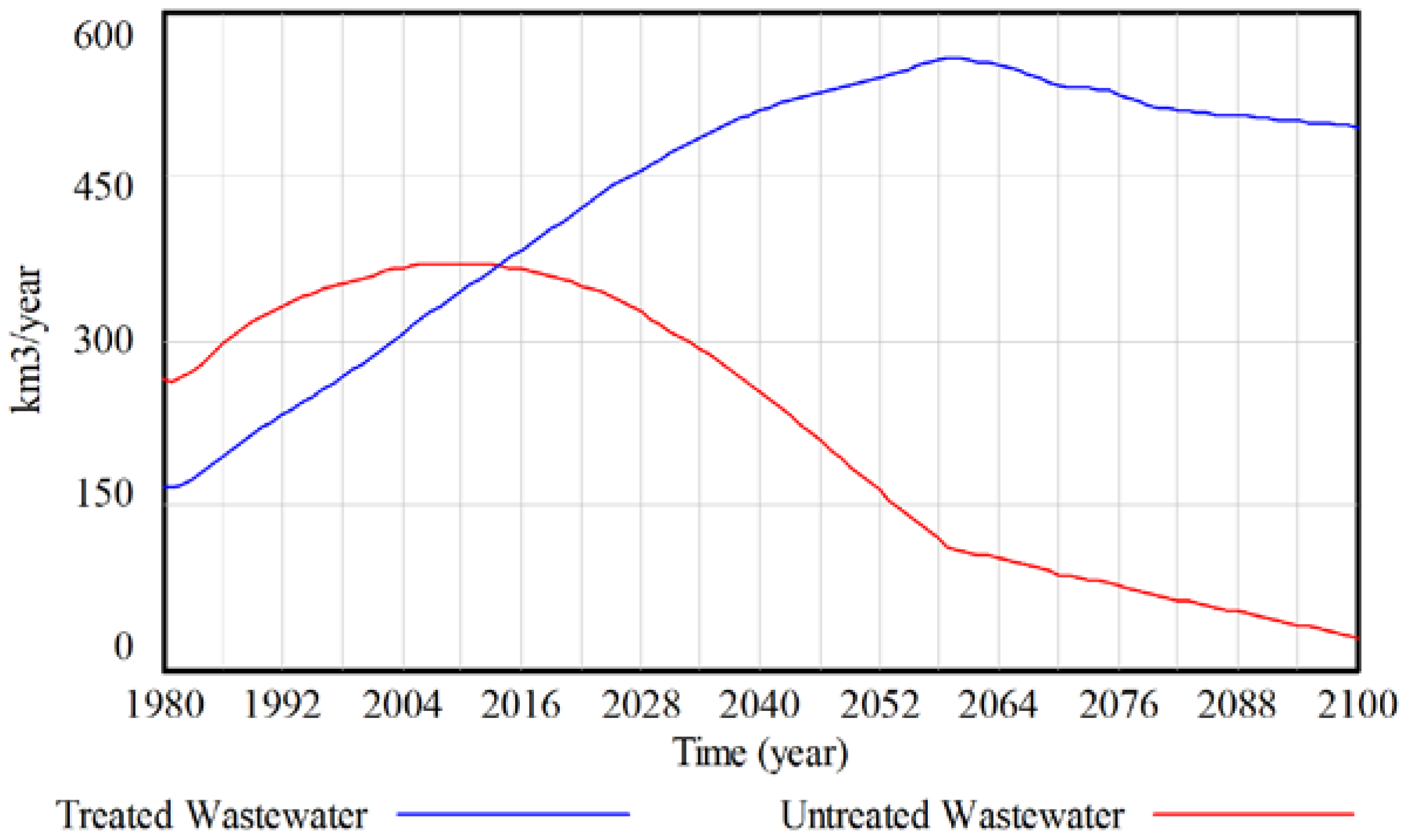
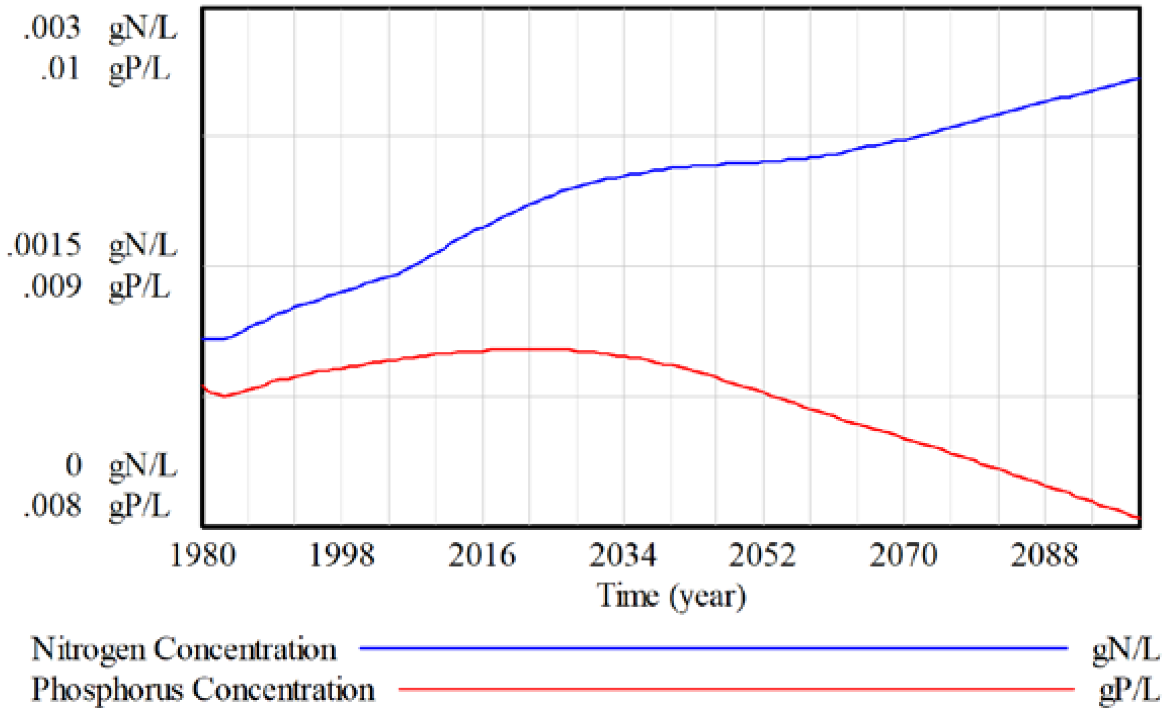
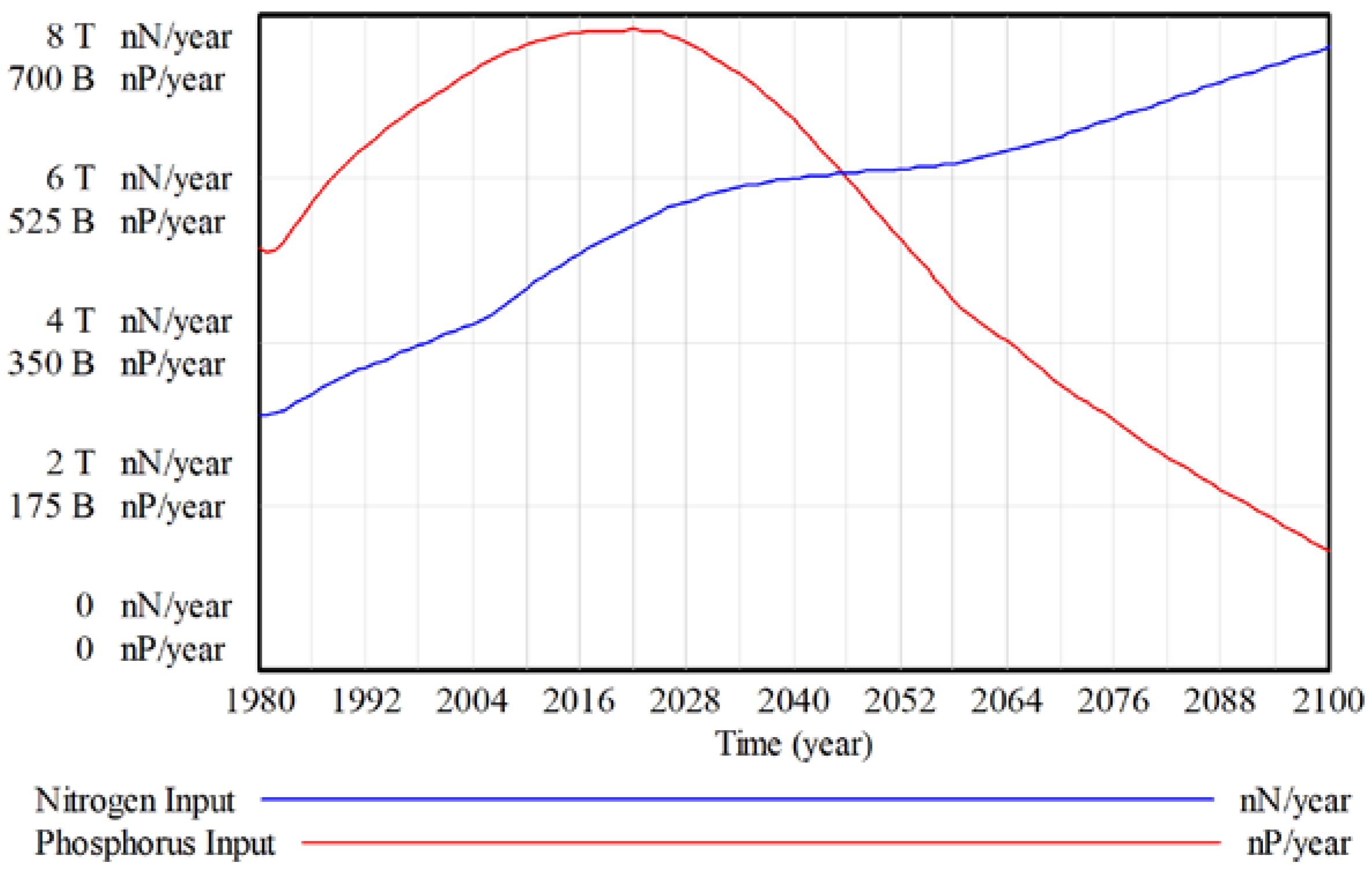
In ANEMI3, nutrient concentrations in surface waters are used as an indicator of water quality on a global scale [
19,
20,
22]. Wastewater and agricultural inputs are used as the main contributors to water quality degradation and changes in the levels of nutrients in the form of total nitrogen and phosphorus are used as indicators of water quality from the nutrient cycle sector of the model. The ratio of current to initial nutrient concentrations for surface water resources is used as a multiplier on the water supply price,
where
= Water supply price for surface water
;
= Producer price for surface water
;
NCE = Nutrient concentration effect
;
= Initial nutrient concentration effect
;
= Influence of water quality on surface water supply price.
The nutrient concentration effect takes into consideration the concentration of both total nitrogen and phosphorus,
where
= Nitrogen content of river stock [nN];
= Phosphorus content of river stock [nP];
SF = Streamflow
.


