Population Characteristics of the Mid-Littoral Chthamalid Barnacle C. stellatus (Poli, 1791) in Eastern Mediterranean (Central Greece)


Abstract
1. Introduction
2. Materials and Methods
2.1. Study Area
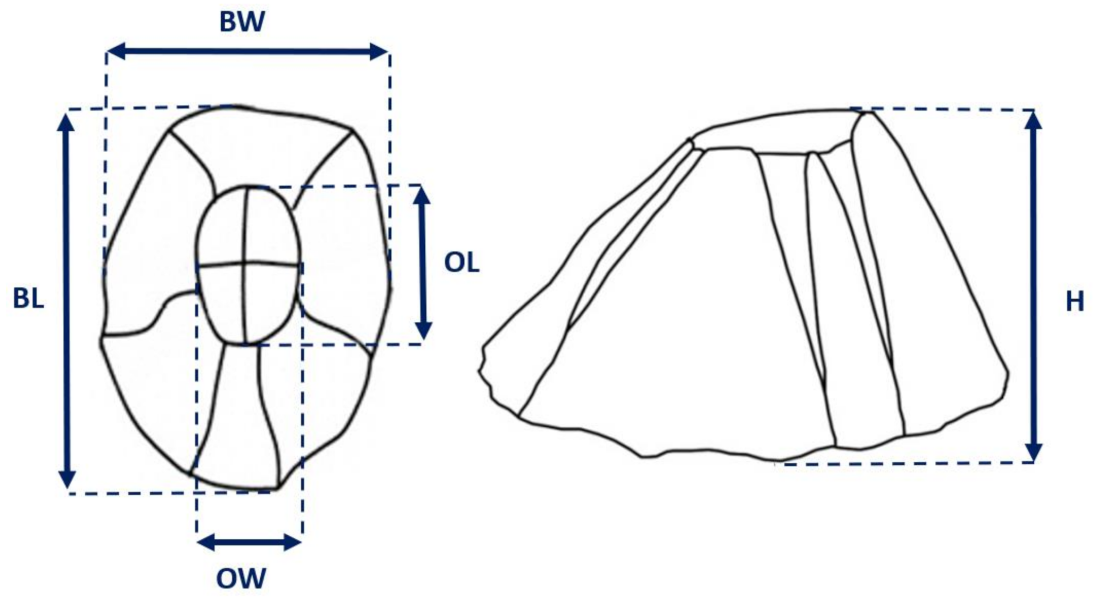
2.2. Field Sampling
2.3. Data Analysis
3. Results
3.1. Physico-Chemical Measurements
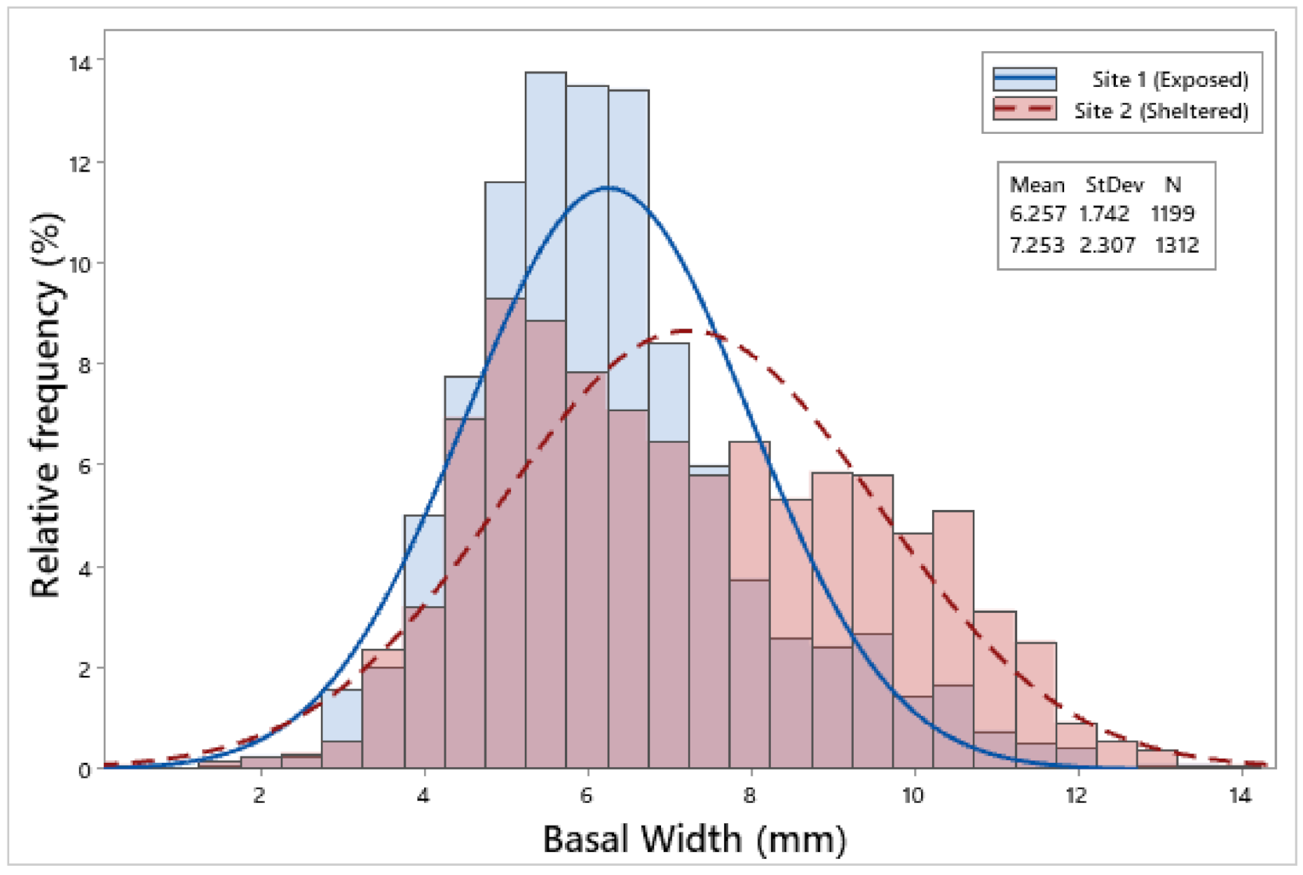
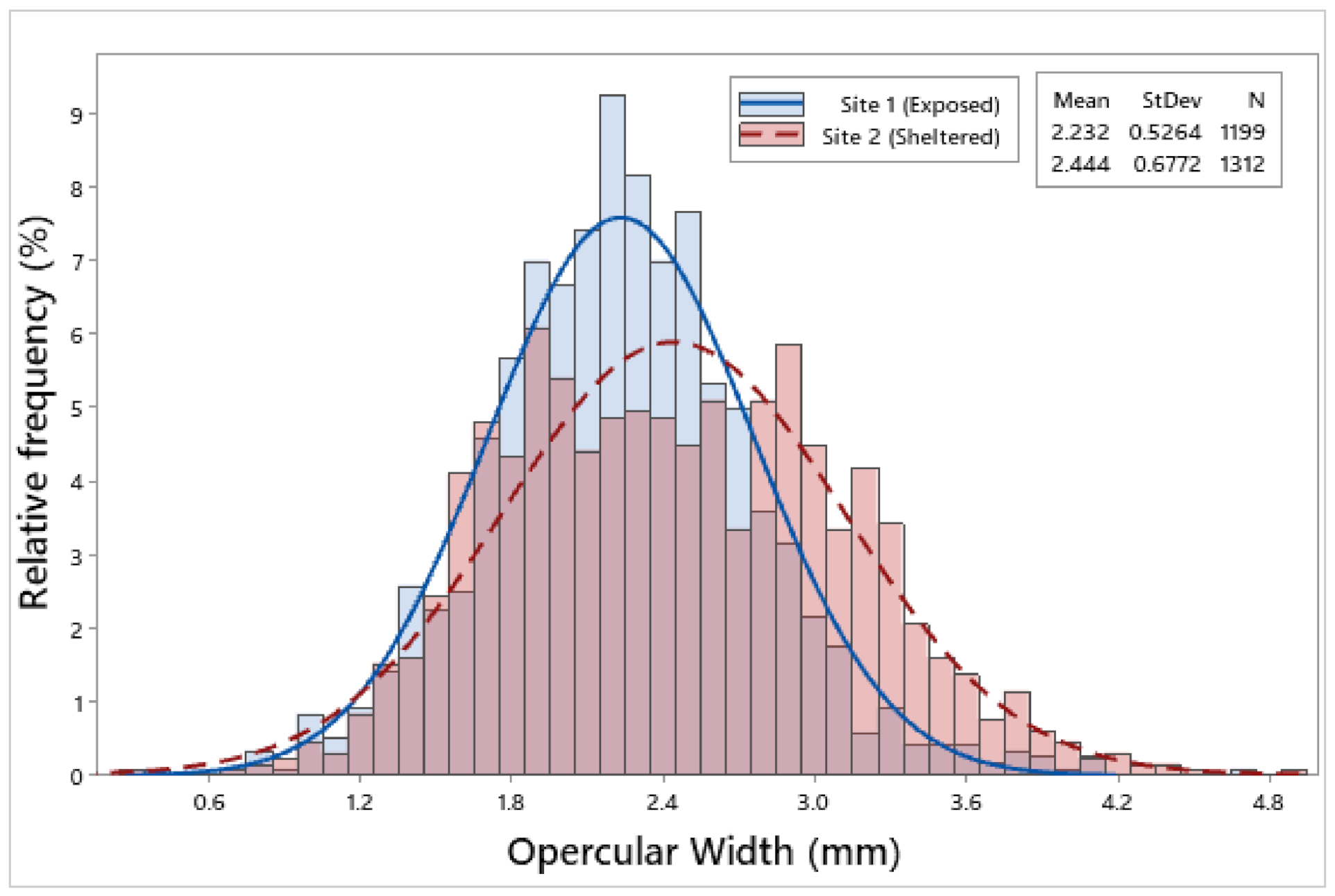
3.2. Biometric Relationships
3.3. Allometric Relationships
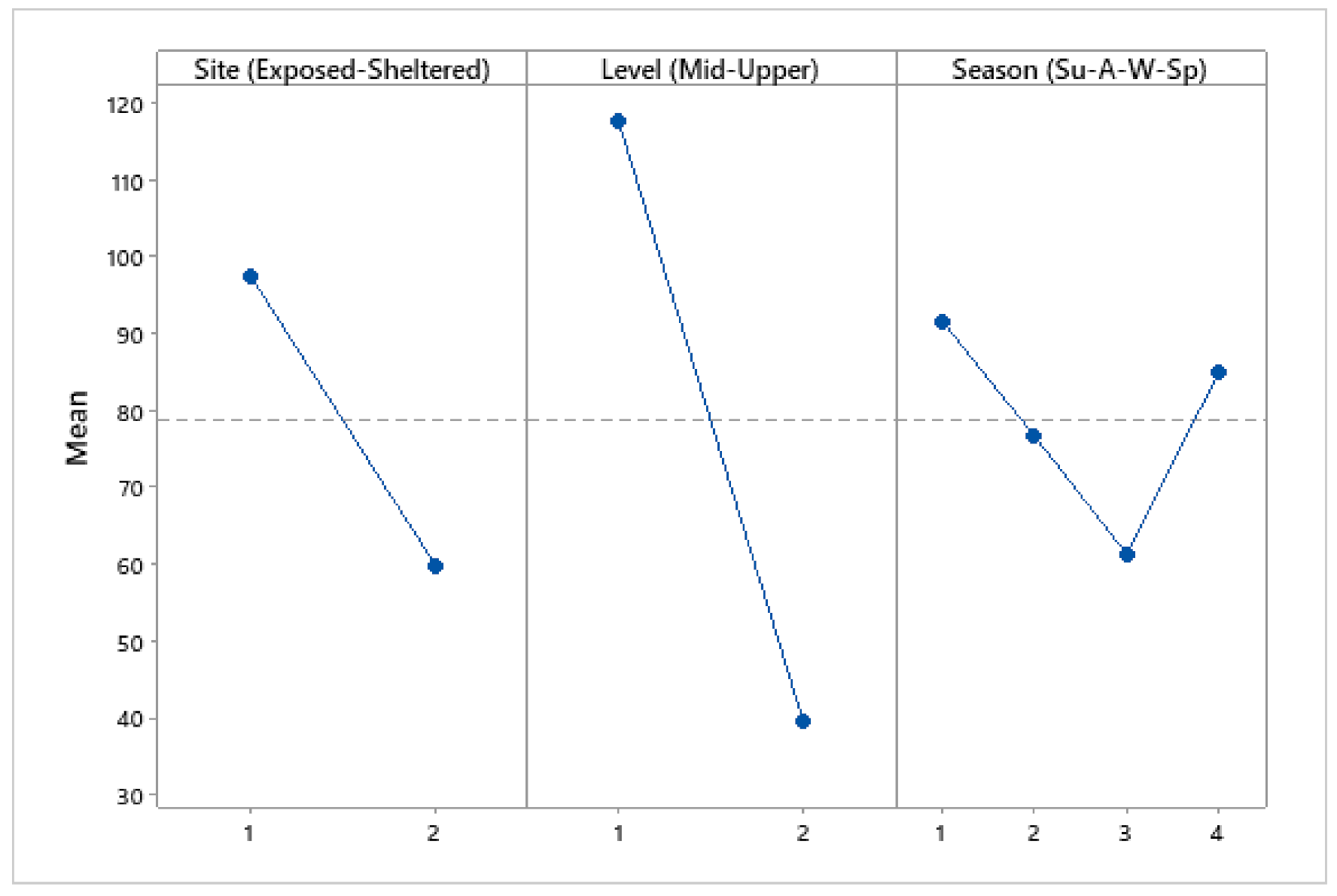
3.4. Population Density
3.5. Distribution Pattern
3.6. Age Composition
4. Discussion
4.1. Biometric Relationships
4.2. Allometric Relationships
4.3. Population Density
4.4. Distribution Pattern
4.5. Age Composition
Author Contributions
Funding
Conflicts of Interest
References
- Stephenson, T.A.; Stephenson, A. Life Between Tidemarks on Rocky Shores; W.H. Freeman and Co.: San Francisco, CA, USA, 1972. [Google Scholar]
- Crisp, D.J.; Southward, A.J.; Southward, E.C. On the distribution of the intertidal barnacles Chthamalus stellatus, Chthamalus montagui and Euraphia depressa. J. Mar. Biol. Assoc. UK 1981, 61, 359–380. [Google Scholar] [CrossRef]
- Williams, G. Distribution of Chthamalus stellatus on the shores of North-East Ireland. Nature 1950, 166, 311. [Google Scholar] [CrossRef] [PubMed]
- Pannacciulli, F.G.; Relini, G. The vertical distribution of Chthamalus montagui and Chthamalus stellatus (Crustacea, Cirripedia) in two areas of the NW Mediterranean Sea. Hydrobiologia 2000, 426, 105–112. [Google Scholar] [CrossRef]
- Sousa, E.B.; Cruz, T.; Castro, J.J. Distribution and abundance of co-occurring chthamalid barnacles Chthamalus montagui and Chthamalus stellatus (Crustacea, Cirripedia) on the southwest coast of Portugal. Hydrobiologia 2000, 440, 339–345. [Google Scholar] [CrossRef]
- Dolenc-Orbanić, N.; Battelli, C. The vertical distribution and abundance of Chthamalus stellatus Poli and Chthamalus montagui Southward (Crustacea, Cirripedia) at two localities of the Istrian peninsula coast (North Adriatic). Acta Adriat. 2017, 58. [Google Scholar] [CrossRef]
- Southward, A.J. On the European species of Chthamalus (Cirripedia). Crustaceana 1964, 6, 241–254. [Google Scholar] [CrossRef]
- Dando, P.R.; Crisp, A.J. Enzyme variation in Chthamalus stellatus and Chthamalus montagui (Crustacea: Cirripedia): Evidence for the presence of C. montagui in the Adriatic. J. Mar. Biol. Assoc. UK 1979, 59, 307–320. [Google Scholar] [CrossRef]
- Anderson, D.T. Barnacles: Structure, Function, Development and Evolution; Chapman and Hall: London, UK, 1994; p. 357. [Google Scholar]
- Ballantine, W.J. A biologically-defined exposure scale for the comparative description of rocky shores. Field Stud. 1961, 1, 1–19. [Google Scholar]
- Southward, A.J. On the taxonomic status and distribution of Chthamalus stellatus (Cirripedia) in the north-east Atlantic region: With a key to the common intertidal barnacles of Britain. J. Mar. Biol. Assoc. UK 1976, 56, 1007–1028. [Google Scholar] [CrossRef]
- Power, A.M. The Ecology of Chthamalid Barnacles: An Evaluation of Settlement and Recruitment in Regulating the Intertidal Distribution of Chthamalus Stellatus and C. Montagui in South-West Ireland. Ph.D. Thesis, National University of Ireland, Cork, Ireland, 2000. [Google Scholar]
- Delany, J.; Myers, A.A.; McGrath, D.; O’Riordan, R.M.; Power, A.M. Role of post-settlement mortality and ’supply-side’ ecology in setting patterns of intertidal distribution in the chthamalid barnacles Chthamalus montagui and C. stellatus. Mar. Ecol. Prog. Ser. 2003, 249, 207–214. [Google Scholar] [CrossRef]
- Jenkins, S.R. Larval habitat selection, not larval supply, determines settlement patterns and adult distribution in two chthamalid barnacles. J. Anim. Ecol. 2005, 74, 893–904. [Google Scholar] [CrossRef]
- Shemesh, E.; Huchon, D.; Simon-Blecher, N.; Achituv, Y. The distribution and molecular diversity of the Eastern Atlantic and Mediterranean chthamalids (Crustacea, Cirripedia). Zool. Scr. 2009, 38, 365–378. [Google Scholar] [CrossRef]
- Dando, P.R.; Southward, A.J. A new species of Chthamalus (Crustacea: Cirripedia) characterized by enzyme electrophoresis and shell morphology: With a revision of other species of Chthamalus from the western shores of the atlantic ocean. J. Mar. Biol. Assoc. UK 1980, 60, 787–831. [Google Scholar] [CrossRef]
- Lavie, B.; Achituv, Y.; Nevo, E. The niche-width variation hypothesis reconfirmed: Validation by genetic diversity in the sessile intertidal cirripedes Chthamalus stellatus and Euraphia depressa (Crustacea, Chthamalidae). J. Zool. Syst. Evol. Res. 1993, 31, 110–118. [Google Scholar] [CrossRef]
- Lipkin, Y.; Safriel, U. Intertidal zonation on Rocky Shores at Mikhmoret (Mediterranean, Israel). J. Ecol. 1971, 59, 1–30. [Google Scholar] [CrossRef]
- O’Riordan, R.M.; Power, A.M.; Myers, A.A. Factors, at different scales, affecting the distribution of species of the genus Chthamalus Ranzani (Cirripedia, Balanomorpha, Chthamaloidea). J. Exp. Mar. Biol. Ecol. 2010, 392, 46–64. [Google Scholar] [CrossRef]
- Guy-Haim, T.; Rilov, G.; Achituv, Y. Different settlement strategies explain intertidal zonation of barnacles in the Eastern Mediterranean. J. Exp. Mar. Biol. Ecol. 2015, 463, 125–134. [Google Scholar] [CrossRef]
- Sanford, E.; Menge, B.A. Spatial and temporal variation in barnacle growth in a coastal upwelling system. Mar. Ecol. Prog. Ser. 2001, 209, 143–157. [Google Scholar] [CrossRef]
- Benedetti-Cecchi, L.; Acunto, S.; Bulleri, F.; Cinelli, F. Population ecology of the barnacle Chthamalus stellatus in the northwest Mediterranean. Mar. Ecol. Prog. Ser. 2000, 198, 157–170. [Google Scholar] [CrossRef]
- Bertness, M.D.; Gaines, S.D.; Yeh, S.M. Making mountains out of barnacles: The dynamics of acorn barnacle hummocking. Ecology 1998, 79, 1382–1394. [Google Scholar] [CrossRef]
- Barnes, H.; Powell, H.T. The development, general morphology, and subsequent elimination of barnacle populations, Balanus crenatus and B. balanoides, after a heavy initial settlement. J. Anim. Ecol. 1950, 19, 175–179. [Google Scholar] [CrossRef]
- Bertness, M.D. Intraspecific competition and facilitation in a northern acorn barnacle population. Ecology 1989, 70, 257–268. [Google Scholar] [CrossRef]
- Crisp, D.J.; Barnes, H. The orientation and distribution of barnacles at settlement with particular reference to surface contour. J. Anim. Ecol. 1954, 23, 142–162. [Google Scholar] [CrossRef]
- Hills, J.M.; Thomason, J.C. The effect of scales of surface roughness on the settlement of barnacle (Semibalanus balanoides) cyprids. Biofouling 1998, 12, 57–69. [Google Scholar] [CrossRef]
- Herbert, R.J.H.; Hawkins, S.J. Effect of rock type on the recruitment and early mortality of the barnacle Chthamalus montagui. J. Exp. Mar. Biol. Ecol. 2006, 334, 96–108. [Google Scholar] [CrossRef]
- Coombes, M.A.; La Marca, E.C.; Naylor, L.A.; Thompson, R.C. Getting into the groove: Opportunities to enhance the ecological value of hard coastal infrastructure using fine-scale surface textures. Ecol. Eng. 2015, 77, 314–323. [Google Scholar] [CrossRef]
- Paine, R.T. Barnacle ecology: Is competition important? The forgotten roles of disturbance and predation. Paleobiology 1981, 7, 553–560. [Google Scholar] [CrossRef]
- Menge, B.A.; Sutherland, J.P. Community regulation: Variation in disturbance, competition, and predation in relation to environmental stress and recruitment. Am. Nat. 1987, 130, 730–757. [Google Scholar] [CrossRef]
- Southward, A.J. Note on the temperature tolerances of some intertidal animals in relation to environmental temperatures and geographical distribution. J. Mar. Biol. Assoc. UK 1958, 37, 49–66. [Google Scholar] [CrossRef]
- Power, A.M.; Myers, A.A.; O’Riordan, R.M.; McGrath, D.; Delany, J. An investigation into rock surface wetness as a parameter contributing to the distribution of the intertidal barnacles Chthamalus stellatus and Chthamalus montagui. Estuar. Coast. Shelf Sci. 2001, 52, 349–356. [Google Scholar] [CrossRef]
- Bertness, M.D.; Gaines, S.D.; Wahle, R.A. Wind-driven settlement patterns in the acorn barnacle Semibalanus balanoides. Mar. Ecol. Prog. Ser. 1996, 137, 103–110. [Google Scholar] [CrossRef]
- Connell, J.H. The influence of interspecific competition and other factors on the distribution of the barnacle Chthamalus stellatus. Ecology 1961, 42, 710–723. [Google Scholar] [CrossRef]
- Wethey, D.S. Sun and shade mediate competition in the barnacles Chthamalus and Semibalanus: A field experiment. Biol. Bull. 1984, 167, 176–185. [Google Scholar] [CrossRef]
- Canessa, M.; Bavestrello, G.; Bo, M.; Betti, F.; Gaggero, L.; Cattaneo-Vietti, R. The influence of the rock mineralogy on population density of Chthamalus (Crustacea: Cirripedia) in the Ligurian Sea (NW Mediterranean Sea). Eur. Zool. J. 2019, 86, 389–401. [Google Scholar] [CrossRef]
- Kitsos, M. Contribution to the Study of the Biodiversity of the Midlittoral and Supralittoral Hard Substratum Assemblages. Ph.D. Thesis, University of Thessaloniki, Thessaloniki, Greece, 2003. [Google Scholar]
- Beşir, C.; Çınar, M.E. Thoracic cirripeds (Thoracica: Cirripedia) from Antalya Bay (eastern Mediterranean). J. Black Sea/Mediterr. Environ. 2012, 18, 251–270. [Google Scholar]
- Shkedy, Y.; Safriel, U.N.; Keasar, T. Life-history of Balanus amphitrite and Chthamalus stellatus recruited to settlement panels in the Mediterranean coast of Israel. Isr. J. Ecol. Evol. 1995, 41, 147–161. [Google Scholar] [CrossRef]
- Vafidis, D.; Antoniadou, C.; Chintiroglou, C. Population dynamics, allometric relationships and reproductive status of Microcosmus sabatieri (Tunicata: Ascidiacea) in the Aegean Sea. J. Mar. Biol. Assoc. UK 2008, 88, 1043–1051. [Google Scholar] [CrossRef]
- Antoniadou, C.; Vafidis, D. Population structure and morphometric relationships of Paracentrotus lividus (Echinodermata: Echinoidea) in the South Aegean Sea. Cah. Biol. Mar. 2009, 50, 293–301. [Google Scholar]
- Kazanidis, G.; Antoniadou, C.; Lolas, A.P.; Neofitou, N.; Vafidis, D.; Chintiroglou, C.; Neofitou, C. Population dynamics and reproduction of Holothuria tubulosa (Holothuroidea: Echinodermata) in the Aegean Sea. J. Mar. Biol. Assoc. UK 2010, 90, 895–901. [Google Scholar] [CrossRef]
- Vafidis, D.; Antoniadou, C.; Voultsiadou, E.; Chintiroglou, C. Population structure of the protected fan mussel Pinna nobilis in the south Aegean Sea (eastern Mediterranean). J. Mar. Biol. Assoc. UK 2014, 94, 787–796. [Google Scholar] [CrossRef]
- Konstantinidis, I.; Gkafas, G.; Karamitros, G.; Lolas, A.; Antoniadou, C.; Vafidis, D.; Exadactylos, A. Population structure of two benthic species with different larval stages in the eastern Mediterranean Sea. J. Environ. Prot. Ecol. 2017, 18, 930–939. [Google Scholar]
- Vafidis, D.; Antoniadou, C.; Ioannidi, V. Population density, size structure, and reproductive cycle of the comestible sea urchin Sphaerechinus granularis (Echinodermata: Echinoidea) in the Pagasitikos Gulf (Aegean Sea). Animals 2020, 10, 1506. [Google Scholar] [CrossRef] [PubMed]
- Vafidis, D.; Drosou, I.; Dimitriou, K.; Klaoudatos, D. Population characteristics of the limpet Patella caerulea (Linnaeus, 1758) in Eastern Mediterranean (Central Greece). Water 2020, 12, 1186. [Google Scholar] [CrossRef]
- Lolas, A.; Vafidis, D. Population dynamics of two caprellid species (Crustaceae: Amphipoda: Caprellidae) from shallow hard bottom assemblages. Mar. Biodivers. 2013, 43, 227–236. [Google Scholar] [CrossRef]
- Lolas, A.; Antoniadou, C.; Vafidis, D. Spatial variation of molluscan fauna associated with Cystoseira assemblages from a semi-enclosed gulf in the Aegean Sea. Reg. Stud. Mar. Sci. 2018, 19, 17–24. [Google Scholar] [CrossRef]
- Triantafyllou, G.; Petihakis, G.; Dounas, C.; Theodorou, A. Assessing marine ecosystem response to nutrient inputs. Mar. Pollut. Bull. 2001, 43, 175–186. [Google Scholar] [CrossRef]
- Friligos, N. Eutrophication assessment in Greek coastal waters. Toxicol. Environ. Chem. 1987, 15, 185–196. [Google Scholar] [CrossRef]
- Korres, G.; Triantafyllou, G.; Petihakis, G.; Raitsos, D.E.; Hoteit, I.; Pollani, A.; Colella, S.; Tsiaras, K. A data assimilation tool for the Pagasitikos Gulf ecosystem dynamics: Methods and benefits. J. Mar. Syst. 2012, 94, S102–S117. [Google Scholar] [CrossRef]
- Petihakis, G.; Triantafyllou, G.; Pollani, A.; Koliou, A.; Theodorou, A. Field data analysis and application of a complex water column biogeochemical model in different areas of a semi-enclosed basin: Towards the development of an ecosystem management tool. Mar. Environ. Res. 2005, 59, 493–518. [Google Scholar] [CrossRef]
- Petihakis, G.; Triantafyllou, G.; Korres, G.; Pollani, A.; Theodorou, A. Ecosystem modeling: Towards the development of a management tool for a marine coastal system: Part I: General circulation, hydrological and dynamical structure. J. Mar. Syst. 2012, 94, S34–S48. [Google Scholar] [CrossRef]
- Bakus, G.J. Quantitative Ecology and Marine Biology; AA Balkema: Rotterdam, The Netherlands, 1990; p. 157. [Google Scholar]
- Abràmoff, M.D.; Magalhães, P.J.; Ram, S.J. Image processing with ImageJ. Biophotonics Int. 2004, 11, 36–42. [Google Scholar]
- Underwood, A.J. Experiments in Ecology: Their Logical Design and Interpretation Using Analysis of Variance; Cambridge University Press: Cambridge, UK, 1997; p. 504. [Google Scholar]
- Sneath, P.H.A.; Sokal, R.R. Numerical Taxonomy. The Principles and Practice of Numerical Classification; W.H. Freeman and Company: San Francisco, CA, USA, 1973; p. 573. [Google Scholar]
- Bray, J.R.; Curtis, J.T. An ordination of the upland forest communities of Southern Wisconsin. Ecol. Monogr. 1957, 27, 326–349. [Google Scholar] [CrossRef]
- Clarke, K.R.; Gorley, R.; Somerfield, P.J.; Warwick, R. Change in Marine Communities: An Approach to Statistical Analysis and Interpretation, 3rd ed.; Primer-E Ltd.: Plymouth, UK, 2014. [Google Scholar]
- Field, J.G.; Clarke, K.R.; Warwick, R.M. A practical strategy for analyzing multispecies distribution patterns. Mar. Ecol. Prog. Ser. 1982, 8, 37–52. [Google Scholar] [CrossRef]
- Morisita, M. Measuring of the dispersion of individuals and analysis of the distributional patterns. Mem. Fac. Sci. Kyushu Univ. Ser. E Biol. 1959, 2, 215–235. [Google Scholar]
- Elliott, J.M. Some Methods for the Statistical Analysis of Samples of Benthic Invertebrates, 2nd ed.; Freshwater Biological Association: Tolouse, France, 1977; p. 156. [Google Scholar]
- Morisita, M. Iσ-Index, a measure of dispersion of individuals. Res. Popul. Ecol. 1962, 4, 1–7. [Google Scholar] [CrossRef]
- Dale, M.R.T.; Dixon, P.; Fortin, M.-J.; Legendre, P.; Myers, D.E.; Rosenberg, M.S. Conceptual and mathematical relationships among methods for spatial analysis. Ecography 2002, 25, 558–577. [Google Scholar] [CrossRef]
- Bhattacharya, C.G. A simple method of resolution of a distribution into Gaussian components. Biometrics 1967, 23, 115–135. [Google Scholar] [CrossRef]
- Gayanilo, F.; Sparre, P.; Pauly, D. FAO-ICLARM Stock Assessment Tools II (FiSAT II) User’s Guide; FAO: Rome, Italy, 2005; p. 168. [Google Scholar]
- Lewis, J.R. The Ecology of Rocky Shores; English Universities Press: London, UK, 1964; p. 323. [Google Scholar]
- Hartnoll, R.G.; Hawkins, S.J. Patchiness and fluctuations on moderately exposed rocky shores. Ophelia 1985, 24, 53–63. [Google Scholar] [CrossRef]
- Jenkins, S.R.; Norton, T.A.; Hawkins, S.J. Settlement and post-settlement interactions between Semibalanus balanoides (L.) (Crustacea: Cirripedia) and three species of fucoid canopy algae. J. Exp. Mar. Biol. Ecol. 1999, 236, 49–67. [Google Scholar] [CrossRef]
- Bellan-Santini, D.; Lacaze, J.-C.; Poizat, C.; Pérès, J.-M. Les Biocénoses Marines et Littorales de Méditerranée, Synthèse, Menaces et Perspectives; Muséum National d’Histoire Naturelle: Paris, France, 1994; p. 246. [Google Scholar]
- Benedetti-Cecchi, L.; Menconi, M.; Cinelli, F. Pre-emption of the substratum and the maintenance of spatial pattern on a rocky shore in the northwest Mediterranean. Mar. Ecol. Prog. Ser. 1999, 181, 13–23. [Google Scholar] [CrossRef][Green Version]
- Pitacco, V.; MavriČ, B.; Orlando-Bonaca, M.; Lipej, L. Rocky macrozoobenthos mediolittoral community in the Gulf of Trieste (North Adriatic) along a gradient of hydromorphological modifications. Acta Adriat. 2013, 54, 67–85. [Google Scholar]
- Caffey, H.M. Spatial and temporal variation in settlement and recruitment of intertidal barnacles. Ecol. Monogr. 1985, 55, 313–332. [Google Scholar] [CrossRef]
- Gaines, S.; Roughgarden, J. Larval settlement rate: A leading determinant of structure in an ecological community of the marine intertidal zone. Proc. Natl. Acad. Sci. USA 1985, 82, 3707–3711. [Google Scholar] [CrossRef] [PubMed]
- Menge, B.A. Relative importance of recruitment and other causes of variation in rocky intertidal community structure. J. Exp. Mar. Biol. Ecol. 1991, 146, 69–100. [Google Scholar] [CrossRef]
- Crisp, D.J. Factors influencing growth-rate in Balanus balanoides. J. Anim. Ecol. 1960, 29, 95–116. [Google Scholar] [CrossRef]
- Bertness, M.D.; Gaines, S.D.; Bermudez, D.; Sanford, E. Extreme spatial variation in the growth and reproductive output of the acorn barnacle Semibalanus balanoides. Mar. Ecol. Prog. Ser. 1991, 75, 91–100. [Google Scholar] [CrossRef]
- Sanford, E.; Bermudez, D.; Bertness, M.D.; Gaines, S.D. Flow, food supply and acorn barnacle population dynamics. Mar. Ecol. Prog. Ser. 1994, 104, 49–62. [Google Scholar] [CrossRef]
- Bustamante, R.H.; Branch, G.M.; Sean, E.; Robertson, B.; Peter, Z.; Michael, S.; Arthur, D.; Nick, H.; Derek, K.; Michelle, J.; et al. Gradients of intertidal productivity around the coast of South Africa and their relationships with consumer biomass. Oecologia 1995, 102, 189–201. [Google Scholar] [CrossRef]
- Leonard, G.H.; Levine, J.M.; Schmidt, P.R.; Bertness, M.D. Flow-driven variation in intertidal community structure in a Maine estuary. Ecology 1998, 79, 1395–1411. [Google Scholar] [CrossRef]
- Schmidt-Nielsen, K. Scaling: Why is Animal Size so Important? Cambridge University Press: Cambridge, UK, 1984; p. 252. [Google Scholar]
- Brown, J.H.; Gillooly, J.F.; Allen, A.P.; Savage, V.M.; West, G.B. Toward a metabolic theory of ecology. Ecology 2004, 85, 1771–1789. [Google Scholar] [CrossRef]
- Woodward, G.; Ebenman, B.; Emmerson, M.; Montoya, J.M.; Olesen, J.M.; Valido, A.; Warren, P.H. Body size in ecological networks. Trends Ecol. Evol. 2005, 20, 402–409. [Google Scholar] [CrossRef] [PubMed]
- Leslie, H.M.; Breck, E.N.; Chan, F.; Lubchenco, J.; Menge, B.A. Barnacle reproductive hotspots linked to nearshore ocean conditions. Proc. Natl. Acad. Sci. USA 2005, 102, 10534–10539. [Google Scholar] [CrossRef] [PubMed]
- Palmer, A.R. Predator size, prey size, and the scaling of vulnerability: Hatching gastropods vs. barnacles. Ecology 1990, 71, 759–775. [Google Scholar] [CrossRef]
- Safriel, U.N.; Erez, N.; Keasar, T. How do limpets maintain barnacle-free submerged artificial surfaces? Bull. Mar. Sci. 1994, 54, 17–23. [Google Scholar]
- Pineda, J. Spatial and temporal patterns in barnacle settlement rate along a southern California rocky shore. Mar. Ecol. Prog. Ser. 1994, 107, 125–138. [Google Scholar] [CrossRef]
- Denley, E.J.; Underwood, A.L. Experiments on factors influencing settlement, survival, and growth of two species of barnacles in new south wales. J. Exp. Mar. Biol. Ecol. 1979, 36, 269–293. [Google Scholar] [CrossRef]
- Foster, B.A. Desiccation as a factor in the intertidal zonation of barnacles. Mar. Biol. 1971, 8, 12–29. [Google Scholar] [CrossRef]
- Walters, L.J.; Wethey, D.S. Settlement and early post-settlement survival of sessile marine invertebrates on topographically complex surfaces: The importance of refuge dimensions and adult morphology. Mar. Ecol. Prog. Ser. 1996, 137, 161–171. [Google Scholar] [CrossRef]
- Knight-Jones, E.W. Laboratory experiments on gregariousness during setting in Balanus balanoides and other barnacles. J. Exp. Biol. 1953, 30, 584–598. [Google Scholar]
- Crisp, D.J. Territorial behaviour in barnacle settlement. J. Exp. Biol. 1961, 38, 429–446. [Google Scholar]
- Crisp, D.J. Gregariousness and systematic affinity in some North Carolinian barnacles. Bull. Mar. Sci. 1990, 47, 516–525. [Google Scholar]
- Raimondi, P.T. Patterns, mechanisms, consequences of variability in settlement and recruitment of an intertidal barnacle. Ecol. Monogr. 1990, 60, 283–309. [Google Scholar] [CrossRef]
- Schubart, C.D.; Basch, L.V.; Miyasato, G. Recruitment of Balanus glandula Darwin (Crustacea: Cirripedia) into empty barnacle tests and its ecological consequences. J. Exp. Mar. Biol. Ecol. 1995, 186, 143–181. [Google Scholar] [CrossRef]
- Roughgarden, J.; Iwasa, Y.; Baxter, C. Demographic theory for an open marine population with space-limited recruitment. Ecology 1985, 66, 54–67. [Google Scholar] [CrossRef]
- Hughes, T.P. Recruitment limitation, mortality, and population regulation in open systems: A case study. Ecology 1990, 71, 12–20. [Google Scholar] [CrossRef]
- Connell, J.H. Effects of competition, predation by Thais lapillus, and other factors on natural populations of the barnacle balanus balanoides. Ecol. Monogr. 1961, 31, 61–104. [Google Scholar] [CrossRef]
- Menge, B.A. Recruitment vs. post recruitment processes as determinants of barnacle population abundance. Ecol. Monogr. 2000, 70, 265–288. [Google Scholar] [CrossRef]
- Carroll, M.L. Barnacle population dynamics and recruitment regulation in southcentral Alaska. J. Exp. Mar. Biol. Ecol. 1996, 199, 285–302. [Google Scholar] [CrossRef]
- Barnes, H. The growth rate of Chthamalus stellatus (Poli). J. Mar. Biol. Assoc. UK 1956, 35, 355–361. [Google Scholar] [CrossRef]
- Deevey, E.S. Life tables for natural populations of animals. Q. Rev. Biol. 1947, 22, 283–314. [Google Scholar] [CrossRef]
- Mieszkowska, N.; Burrows, M.T.; Pannacciulli, F.G.; Hawkins, S.J. Multidecadal signals within co-occurring intertidal barnacles Semibalanus balanoides and Chthamalus spp. linked to the Atlantic Multidecadal Oscillation. J. Mar. Syst. 2014, 133, 70–76. [Google Scholar] [CrossRef]
- Schneider, S.H. What is ‘dangerous’ climate change? Nature 2001, 411, 17–19. [Google Scholar] [CrossRef] [PubMed]
- Southward, A.J.; Boalch, G. The marine resources of Devon’s coastal waters. New Marit. Hist. Devon 1992, 1, 61–71. [Google Scholar]
- Southward, A.J.; Boalch, G. The effect of changing climate on marine life: Past events and future predictions. Exeter Marit. Stud. 1994, 9, 101–143. [Google Scholar]
- Southward, A.J.; Hawkins, S.J.; Burrows, M.T. Seventy years’ observations of changes in distribution and abundance of zooplankton and intertidal organisms in the western English Channel in relation to rising sea temperature. J. Therm. Biol. 1995, 20, 127–155. [Google Scholar] [CrossRef]


| Sampling Period | Site 1 | Site 2 | ||||||
|---|---|---|---|---|---|---|---|---|
| T (°C) | S (psu) | pH | O2 (mg L−1) | T (°C) | S (psu) | pH | O2 (mg L−1) | |
| June | 25.27 | 39.00 | 8.24 | 5.71 | 25.81 | 39.40 | 8.26 | 6.61 |
| July | 27.80 | 39.20 | 8.23 | 5.45 | 27.60 | 39.56 | 8.26 | 5.44 |
| August | 27.50 | 40.05 | 8.31 | 5.02 | 27.31 | 39.50 | 8.26 | 5.06 |
| September | 24.10 | 38.84 | 8.29 | 5.92 | 24.43 | 38.53 | 8.29 | 4.92 |
| October | 20.25 | 38.15 | 8.35 | 5.54 | 19.97 | 38.20 | 8.31 | 5.22 |
| November | 17.90 | 38.15 | 8.39 | 4.67 | 17.95 | 38.72 | 8.34 | 4.48 |
| December | 15.95 | 37.90 | 8.24 | 4.97 | 15.93 | 38.11 | 8.31 | 5.99 |
| January | 13.52 | 37.80 | 8.33 | 4.01 | 13.80 | 38.10 | 8.27 | 5.21 |
| February | 13.45 | 38.15 | 8.27 | 5.11 | 13.46 | 38.33 | 8.28 | 5.04 |
| March | 13.20 | 38.40 | 8.29 | 6.49 | 13.53 | 38.81 | 8.23 | 4.76 |
| April | 16.30 | 38.91 | 8.28 | 6.49 | 15.91 | 38.80 | 8.28 | 6.62 |
| May | 22.70 | 38.82 | 8.26 | 5.48 | 22.50 | 38.87 | 8.29 | 5.88 |
| Sampling Period | No. of Individuals | BL ± SE | BW ± SE | H ± SE | OL ± SE | OW ± SE | Wt ± SE |
|---|---|---|---|---|---|---|---|
| Site | (n) | ||||||
| Site 1 | 1199 | 6.85 ± 0.05 | 6.26 ± 0.05 | 2.75 ± 0.02 | 2.65 ± 0.02 | 2.23 ± 0.01 | 0.09 ± 0.002 |
| Site 2 | 1312 | 7.71 ± 0.06 | 7.25 ± 0.06 | 2.94 ± 0.02 | 2.93 ± 0.02 | 2.44 ± 0.02 | 0.13 ± 0.002 |
| F = 116.65, p < 0.001 | F = 146.88, p < 0.001 | F = 35.17, p < 0.001 | F = 105.98, p < 0.001 | F = 76.00, p < 0.001 | F = 132.13, p < 0.001 | ||
| Season | (n) | ||||||
| Summer | 709 | 7.32 a,b ± 0.07 | 6.75 b ± 0.07 | 2.76 b ± 0.03 | 2.82 a ± 0.03 | 2.36 a ± 0.02 | 0.12 a ± 0.003 |
| Autumn | 539 | 7.22 b,c ± 0.08 | 6.71 b ± 0.08 | 2.88 a,b ± 0.03 | 2.76 a,b ± 0.03 | 2.33 a,b ± 0.02 | 0.11 b,c ± 0.003 |
| Winter | 750 | 7.53 a ± 0.08 | 7.06 a ± 0.08 | 2.97 a ± 0.03 | 2.86 a ± 0.03 | 2.39 a ± 0.02 | 0.12 a,b ± 0.003 |
| Spring | 513 | 6.99 c ± 0.09 | 6.47 b ±0.09 | 2.76 b ± 0.03 | 2.69 b ± 0.03 | 2.24 b ± 0.03 | 0.09 c ± 0.004 |
| F = 7.60, p < 0.001 | F = 8.39, p < 0.001 | F = 10.64, p < 0.001 | F = 6.17, p < 0.001 | F = 6.67, p < 0.001 | F = 10.11, p < 0.001 | ||
| Total | 2511 | 7.29 ± 2.04 | 6.78 ± 2.12 | 2.85 ± 0.86 | 2.79 ± 0.69 | 2.34 ± 0.01 | 0.11 ± 0.09 |
| Morphometric Relationships | Equation Comparison | ||||||
|---|---|---|---|---|---|---|---|
| Sampling Site | Equation | N | R2 | t-test | Allometry | Slopes | Intercepts |
| Site 1 | Wt = 0.000631904 × BL 2.50621 | 1199 | 86.5 | ** | Negative | ** | ** |
| Site 2 | Wt = 0.00119825 × BL 2.25133 | 1312 | 86.7 | ** | Negative | ||
| Site 1 | Wt = 0.00118524 × BW 2.29087 | 1199 | 86.6 | ** | Negative | * | * |
| Site 2 | Wt = 0.00164777 × BW 2.15174 | 1312 | 88.7 | ** | Negative | ||
| Site 1 | Wt = 0.0104422 × H 2.0243 | 1199 | 78.5 | ** | Negative | ns | ** |
| Site 2 | Wt = 0.0159692 × H 1.89858 | 1312 | 76.0 | ** | Negative | ||
| Site 1 | BL = 3.79544 × H 0.59309 | 1199 | 67.7 | ** | Negative | ** | ns |
| Site 2 | BL = 3.58751 × H 0.71623 | 1312 | 72.5 | ** | Negative | ||
| Site 1 | BL = 1.71255 × BW 0.75949 | 1199 | 82.6 | ** | Negative | ns | ns |
| Site 2 | BL = 1.69340 × BW 0.76932 | 1312 | 86.6 | ** | Negative | ||
| Site 1 | BW = 3.47928 × H 0.58979 | 1199 | 61.4 | ** | Negative | ** | * |
| Site 2 | BW = 3.15446 × H 0.77814 | 1312 | 70.7 | ** | Negative | ||
| Site 1 | OL = 1.35775 × OW 0.83600 | 1199 | 90.1 | ** | Negative | ns | ns |
| Site 2 | OL = 1.35591 × OW 0.86603 | 1312 | 92.8 | ** | Negative | ||
| Source of Variation | DF | SS | MS | F | p |
|---|---|---|---|---|---|
| Site (Exposed–Sheltered) | 1 | 34,143 | 34,143 | 31.09 | <0.001 |
| Level (Mid–Upper) | 1 | 146,494 | 146,494 | 133.39 | <0.001 |
| Season | 1 | 1478 | 1478 | 1.35 | 0.249 |
| Error | 92 | 101,039 | 1098 | ||
| Total | 95 | 283,154 |
| Sampling Season | Sites | Shore Level | Population Density (ind/m2 ± SD) | Iδ | X2 | Dispersion Pattern | Significance Level | DF |
|---|---|---|---|---|---|---|---|---|
| Summer | Site 1 | Mid | 19.950 ± 2.907 | 1.01 | 11.73 | random | <0.05 | 5 |
| Site 1 | Upper | 5.574 ± 1.184 | 1.04 | 11.03 | random | ns | 5 | |
| Summer | Site 2 | Mid | 7.841 ±2.823 | 1.05 | 28.78 | random | <0.001 | 5 |
| Site 2 | Upper | 3.289 ± 2.199 | 1.06 | 11.32 | random | <0.05 | 5 | |
| Autumn | Site 1 | Mid | 14.947 ± 4,245 | 1.01 | 4.87 | random | ns | 5 |
| Site 1 | Upper | 4.078 ± 1.623 | 1.01 | 3.05 | random | ns | 5 | |
| Autumn | Site 2 | Mid | 7.696 ± 3.220 | 1.02 | 11.39 | random | <0.05 | 5 |
| Site 2 | Upper | 3.967 ± 2.012 | 1.09 | 16.99 | clustered | <0.001 | 5 | |
| Winter | Site 1 | Mid | 10.969 ± 3.590 | 1.00 | 0.83 | random | ns | 5 |
| Site 1 | Upper | 3.186 ± 686 | 1.07 | 19.86 | clustered | <0.001 | 5 | |
| Winter | Site 2 | Mid | 8.054 ± 1.352 | 1.15 | 55.17 | clustered | <0.001 | 5 |
| Site 2 | Upper | 2.308 ± 1.452 | 1.02 | 2.23 | random | ns | 5 | |
| Spring | Site 1 | Mid | 12.849 ± 2.964 | 1.01 | 11.76 | random | <0.05 | 5 |
| Site 1 | Upper | 6.479 ± 2.737 | 1.02 | 4.90 | random | ns | 5 | |
| Spring | Site 2 | Mid | 11.889 ± 3.473 | 1.00 | 2.95 | random | ns | 5 |
| Site 2 | Upper | 2.813 ± 1.193 | 1.09 | 19.44 | clustered | <0.001 | 5 |
| Age Group | Mean Length (mm) | Standard Deviation | Population Size | Separation Index (SI) | Population % |
|---|---|---|---|---|---|
| 1 | 3.32 | 0.47 | 33 | 1.40 | |
| 2 | 5.07 | 0.57 | 314 | 2.37 | 13.34 |
| 3 | 6.50 | 0.66 | 1059 | 2.07 | 45.01 |
| 4 | 8.10 | 0.57 | 500 | 2.10 | 21.25 |
| 5 | 9.65 | 0.67 | 413 | 2.07 | 17.55 |
| 6 | 12.82 | 0.65 | 34 | 2.36 | 1.44 |
| Area | Average Density (ind/m2) ± SE | References |
|---|---|---|
| Italy Eastern Ligurian | 10,831 ± 2527 | [37] |
| Italy North Adriatic | 514 | [6] |
| Israel Habonim | 7618 ± 628 | [20] |
| Turkey Antalya Bay | 23,470 ± 12,001 | [39] |
| Spain Western Med | 8900 ± 2510 | [2] |
| France Western Med | 32,267 ± 6834 | [2] |
| Greece Chalkida | 1280 | [38] |
| Greece Thermaikos Gulf | 1773 | [38] |
| Greece Chalkidiki | 4594 | [38] |
| Greece Pagasitikos Gulf | 7868 ± 557 | Present study |
Publisher’s Note: MDPI stays neutral with regard to jurisdictional claims in published maps and institutional affiliations. |
© 2020 by the authors. Licensee MDPI, Basel, Switzerland. This article is an open access article distributed under the terms and conditions of the Creative Commons Attribution (CC BY) license (http://creativecommons.org/licenses/by/4.0/).
Share and Cite
Klaoudatos, D.; Kotsiri, Z.; Neofitou, N.; Lolas, A.; Vafidis, D. Population Characteristics of the Mid-Littoral Chthamalid Barnacle C. stellatus (Poli, 1791) in Eastern Mediterranean (Central Greece). Water 2020, 12, 3304. https://doi.org/10.3390/w12123304
Klaoudatos D, Kotsiri Z, Neofitou N, Lolas A, Vafidis D. Population Characteristics of the Mid-Littoral Chthamalid Barnacle C. stellatus (Poli, 1791) in Eastern Mediterranean (Central Greece). Water. 2020; 12(12):3304. https://doi.org/10.3390/w12123304
Chicago/Turabian StyleKlaoudatos, Dimitris, Zoi Kotsiri, Nikos Neofitou, Alexios Lolas, and Dimitris Vafidis. 2020. "Population Characteristics of the Mid-Littoral Chthamalid Barnacle C. stellatus (Poli, 1791) in Eastern Mediterranean (Central Greece)" Water 12, no. 12: 3304. https://doi.org/10.3390/w12123304
APA StyleKlaoudatos, D., Kotsiri, Z., Neofitou, N., Lolas, A., & Vafidis, D. (2020). Population Characteristics of the Mid-Littoral Chthamalid Barnacle C. stellatus (Poli, 1791) in Eastern Mediterranean (Central Greece). Water, 12(12), 3304. https://doi.org/10.3390/w12123304