Sensitivity Analysis of the MOHID-Land Hydrological Model: A Case Study of the Ulla River Basin


Abstract
1. Introduction
2. Materials and Methods
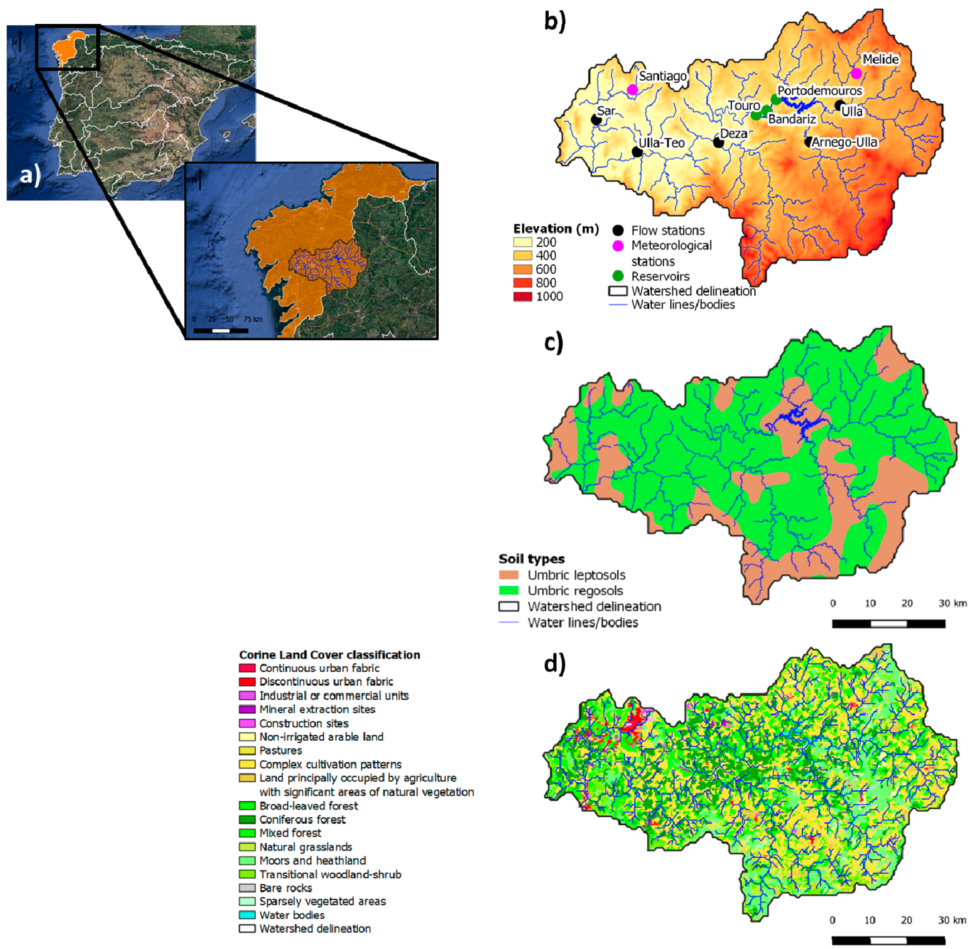
2.1. Description of the Study Area
2.2. Model Description
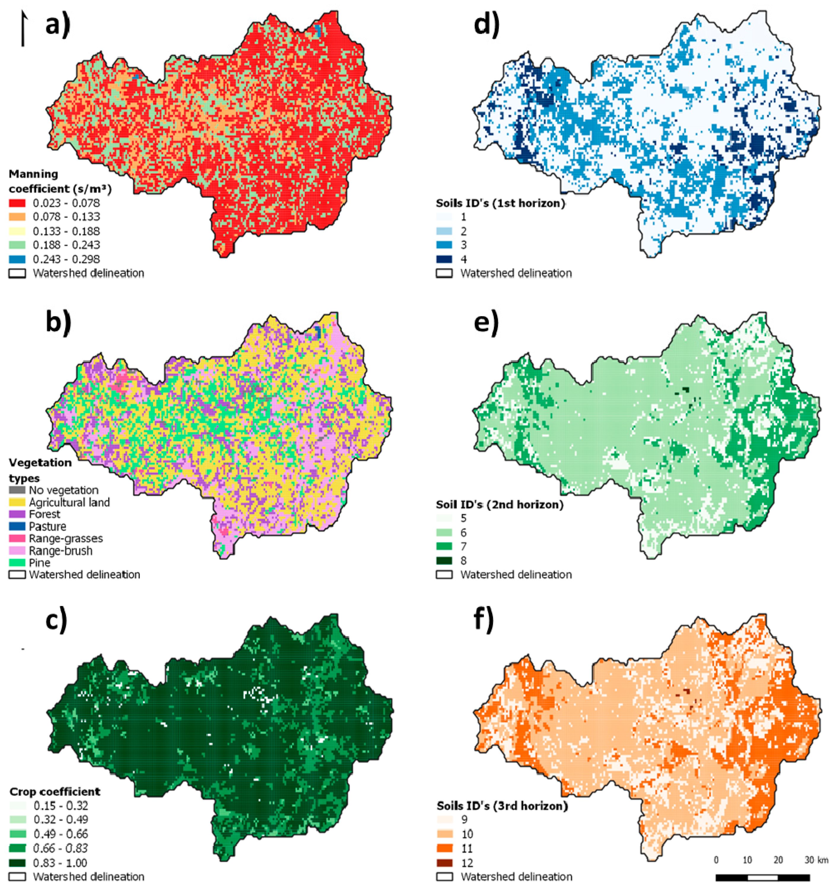
2.2.1. Infiltration
2.2.2. Surface Flow
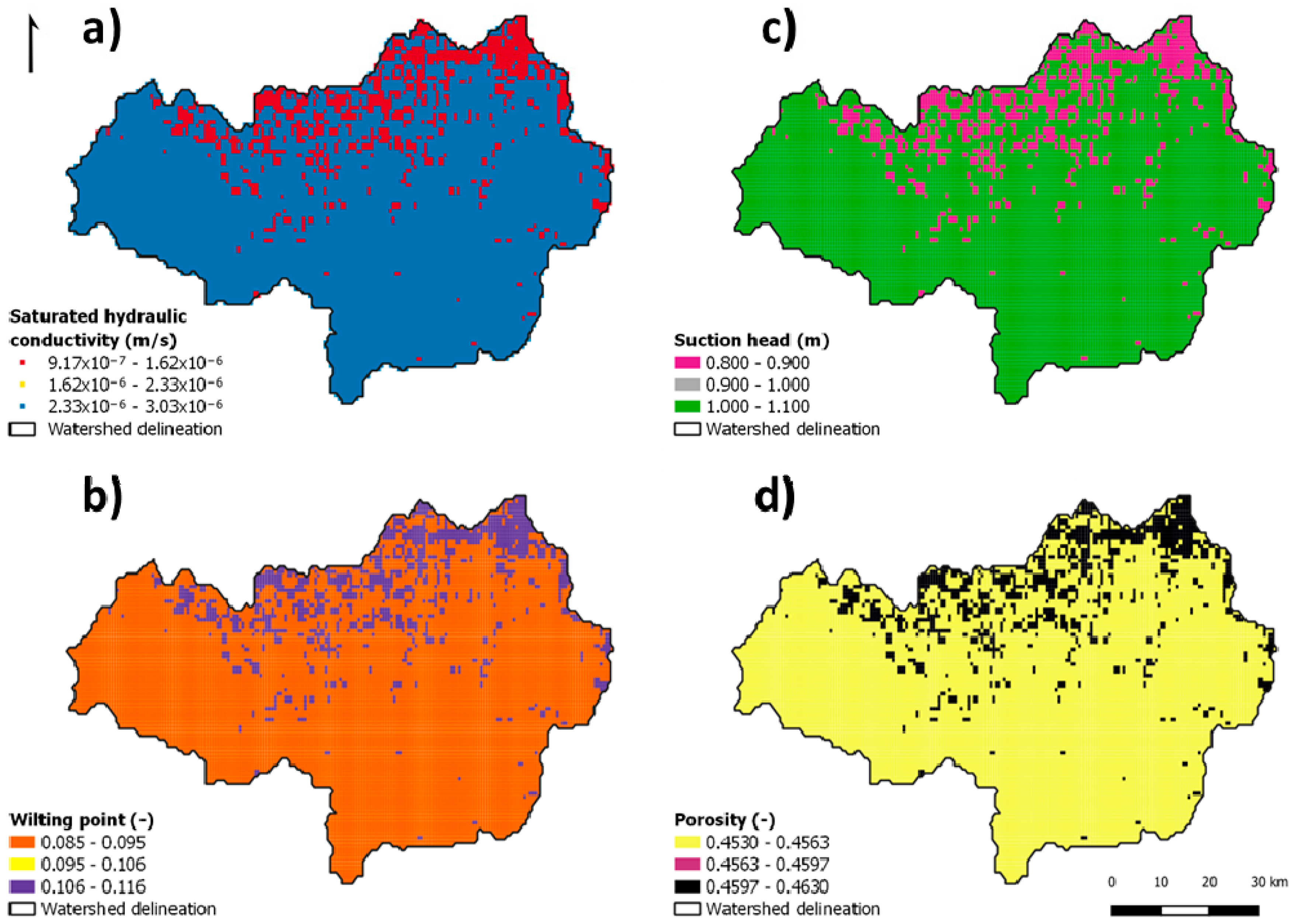
2.2.3. Porous Media
2.2.4. Root Water Uptake
2.3. Model Set-Up (Reference Simulation)
2.4. Sensitivity Analysis
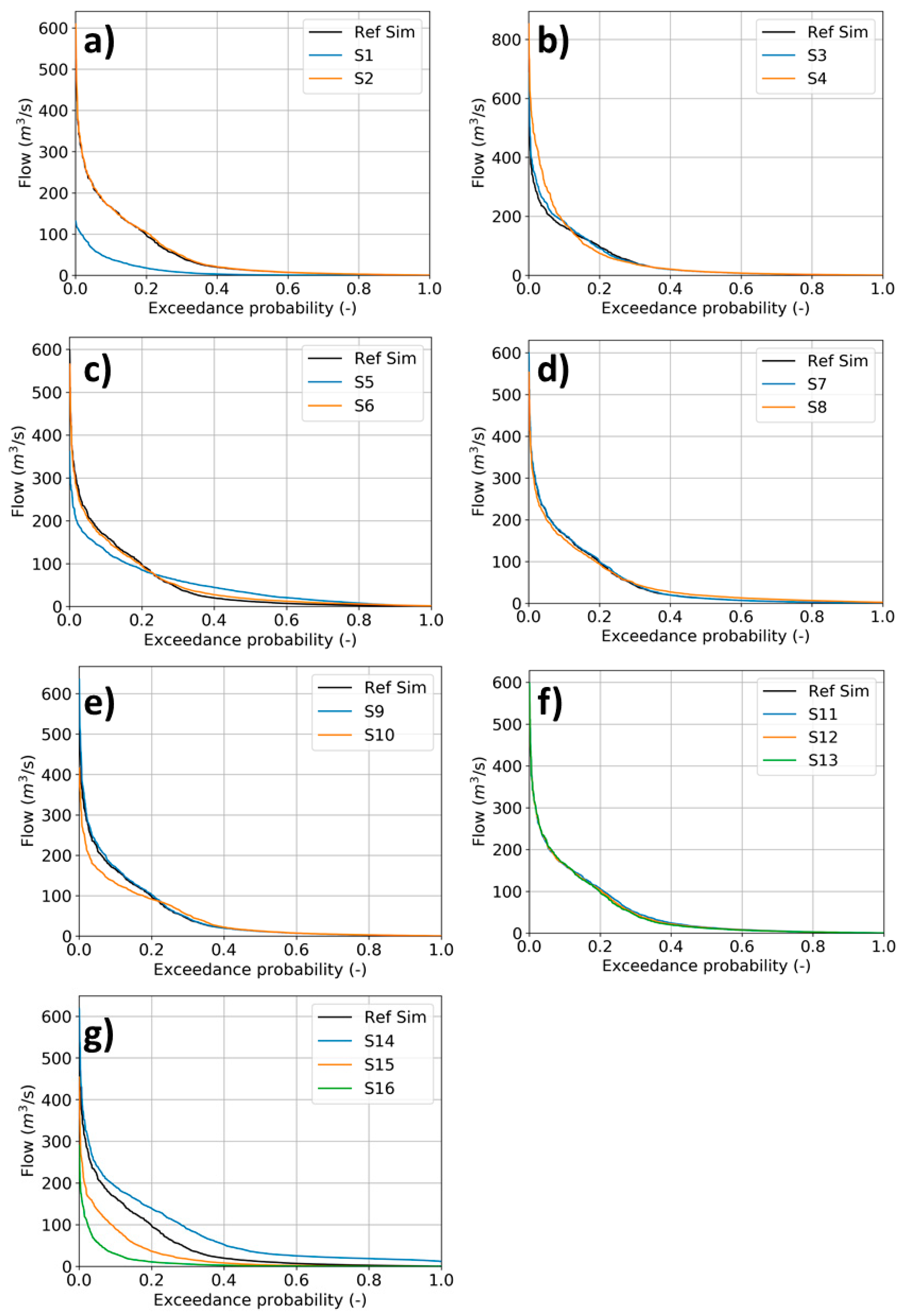
- The resolution of the simulation grid was modified from 0.005° (≈500 m) used in the reference simulation to 0.01° (≈1000 m; 140 columns × 100 rows) (simulation 1, S1).
- The DTM was changed from the EU-DEM (30 m) to the one provided by the National Geographic Institute of Spain, with a resolution of 5 m [55]. The new DTM was interpolated to the simulation grid, with the model also delineating a new catchment area and drainage network based on that input (S2).
- The effect of cross-section geometry on river flow was assessed in two simulations. In one (S3), the top and bottom widths were increased by 25% (i.e., larger river) while the depth and the shape of the cross-section remained the same. In the other (S4), the river depth was increased by 100%, while the top and bottom widths and the shape of the cross-section were maintained as in the default simulation. Table 1 shows the variations introduced to those parameters per drainage area.
- The Ksat value of each cell was multiplied by a factor of 10 while fh was maintained (S5). As a result, the horizontal hydraulic conductivity was also modified since fh = Khor/Kvert.
- The fh value was analyzed in a separate test by changing this parameter from 10, in the reference simulation, to 20 (S6). The Ksat,vert values were the same as in the default scenario, meaning that a change in fh led to an increase in the Khor.
- The number of layers in the vertical grid increased from 6 to 12 as defined in Table 3 (S7), thus decreasing the thickness of the layers when compared with the reference simulation.
- The soil depth also increased from 5 to 10 m (S8), with the number of layers in the vertical grid increasing from six to nine (Table 3).
- The surface Manning coefficients increased by 50% when compared with the reference simulation (S9).
- The channel Manning coefficient also increased from 0.035 s m−1/3 to 0.0525 s m−1/3, corresponding to a 50% increase (S10).
- The SCS curve number method was used to compute runoff and soil water infiltration as an alternative to Equation (1) (S11). The CN values were defined for each grid cell according to the soil type and land cover. The hydrologic soil groups (HSGs) were extracted from the HYSOGs250 m dataset [56], which derived that information from the soil texture classes and depth to bedrock available in the SoilGrids250 m product [57]. That information was then merged with Corine Land Cover [29] data following the United States Department of Agriculture [58] guidelines to derive the CN values. Figure 5 presents the CN values adopted in this study. Additionally, changes in the CN values were also assessed by decreasing the values set in S11 by 25% (S12).
- The Green and Ampt infiltration method was now used as an alternative to Equation (1) (S13). The MOHID-Land model needed the values of Ksat,ver, suction head, porosity, and wilting point in each cell as inputs (Figure 6). These inputs were obtained by combining the information available in the LUCAS database [59] with data from Rossman [60], who related the soil texture classes with the soil hydraulic characteristics.
- The importance of the porous media and vegetation growth processes for river flow results were investigated in three separate simulations. Firstly, vegetation growth processes were deactivated (S14), meaning that no evapotranspiration occurred in the catchment area. Secondly, both the porous media and vegetation growth processes were deactivated (S15). In the absence of porous media, the SCS CN method was used to compute the partitioning of rainfall data between surface runoff and infiltration. Infiltration water was then lost to the system since soil porous processes were not considered. The CN values presented in Figure 5 were adopted for this analysis. Lastly, both porous media and vegetation growth processes remained deactivated, but the CN values were reduced by 25% (S16) as in S12.
2.5. Model Calibration/Validation
3. Results and Discussion
3.1. Impact of Model Parameters/Processes on River Flow
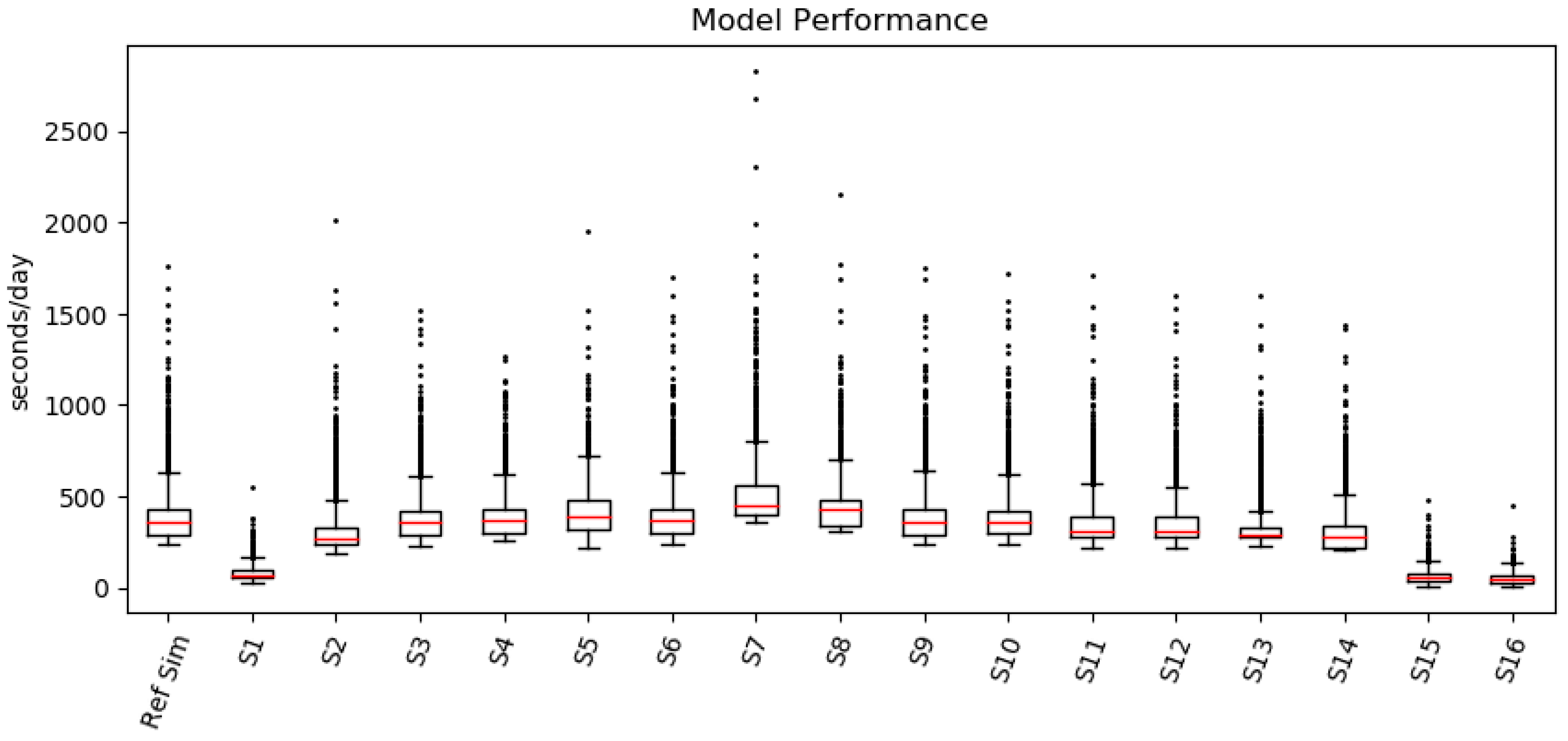
3.2. Impact of Model Parameters/Processes on Model Time Consumption
3.3. Prediction of River Flow in the Ulla River Watershed
4. Conclusions
Author Contributions
Funding
Conflicts of Interest
References
- Wheater, H.; Sorooshian, S.; Sharma, K.D. (Eds.) Hydrological Modelling in Arid and Semi-Arid Areas; International Hydrology Series; Cambridge University Press: Cambridge, UK, 2007; pp. 1–4. [Google Scholar]
- Devi, G.K.; Ganasri, B.P.; Dwarakish, G.S. A review on hydrological models. Aquat. Procedia 2015, 4, 1001–1007. [Google Scholar] [CrossRef]
- Sitterson, J.; Knightes, C.; Parmar, R.; Wolfe, K.; Muche, M.; Avant, B. An Overview of Rainfall-Runoff Model Types; U.S. Environmental Protection Agency: Washington, DC, USA, 2017.
- Fatichi, S.; Vivoni, E.R.; Ogden, F.L.; Ivanov, V.Y.; Mirus, B.; Gochis, D.; Downer, C.W.; Camporese, M.; Davidson, J.H.; Ebel, B.; et al. An overview of current applications, challenges and future trends in distributed process-based models in hydrology. J. Hydrol. 2016, 537, 45–60. [Google Scholar] [CrossRef]
- Abbott, M.B.; Bathurst, J.C.; Cunge, J.A.; O’Connell, P.E.; Rasmussen, J. An introduction to the European Hydrological System, Systeme Hydrologique Europeen, “SHE”, 1: History and philosophy of a physically-based, distributed modelling system. J. Hydrol. 1986, 87, 45–59. [Google Scholar] [CrossRef]
- Abbott, M.B.; Bathurst, J.C.; Cunge, J.A.; O’Connell, P.E.; Rasmussen, J. An introduction to the European Hydrological System, Systeme Hydrologique Europeen, “SHE”, 2: Structure of a physically-based, distributed modelling system. J. Hydrol. 1986, 87, 61–77. [Google Scholar] [CrossRef]
- Ranatunga, T.; Tong, S.T.Y.; Yang, Y.J. An approach to measure parameter sensitivity in watershed hydrological modelling. Hydrol. Sci. J. 2017, 62, 76–92. [Google Scholar] [CrossRef]
- Pianosi, F.; Beven, K.; Freer, J.; Hall, J.; Rougier, J.; Stephenson, D.; Wagener, T. Sensitivity analysis of environmental models: A systematic review with practical workflow. Environ. Model. Softw. 2016, 79, 214–232. [Google Scholar] [CrossRef]
- Silva, M.G.; Netto, A.O.A.; Neves, R.J.J.; Vasco, A.N.; Almeida, C.; Faccioli, G.G. Sensitivity analysis and calibration of hydrological modeling of the watershed Northeast Brazil. J. Environ. Prot. 2015, 6, 837–850. [Google Scholar] [CrossRef]
- Shi, Y.; Xu, G.; Wang, Y.; Engel, B.A.; Peng, H.; Zhang, W.; Cheng, M.; Dai, M. Modelling hydrology and water quality processes in the Pengxi River basin of the Three Gorges Reservoir using the soil and water assessment tool. Agric. Water Manag. 2017, 182, 24–38. [Google Scholar] [CrossRef]
- Song, X.; Zhang, J.; Zhan, C.; Xuan, Y.; Ye, M.; Xu, C. Global sensitivity analysis in hydrological modeling: Review of concepts, methods, theoretical framework, and applications. J. Hydrol. 2015, 523, 739–757. [Google Scholar] [CrossRef]
- Sreedevi, S.; Eldho, T.I. A two-stage sensitivity analysis for parameter identification and calibration of a physically-based distributed model in a river basin. Hydrol. Sci. J. 2019, 64, 701–719. [Google Scholar] [CrossRef]
- Christiaens, K.; Feyen, J. Use of sensitivity and uncertainty measures in distributed hydrological modeling with an application to the MIKE SHE model. Water Resour. Res. 2002, 38. [Google Scholar] [CrossRef]
- Hamby, D.M. A review of techniques for parameter sensitivity. Environ. Monit. Assess. 1994, 32, 135–154. [Google Scholar] [CrossRef]
- Doherty, J.; Hunt, R.J. Two statistics for evaluating parameter identifiability and error reduction. J. Hydrol. 2009, 366, 119–127. [Google Scholar] [CrossRef]
- Trancoso, A.R.; Braunschweig, F.; Leitão, P.C.; Obermann, M.; Neves, R. An advanced modelling tool for simulating complex river systems. Sci. Total Environ. 2009, 407, 3004–3016. [Google Scholar] [CrossRef]
- Ramos, T.B.; Simionesei, L.; Jauch, E.; Almeida, C.; Neves, R. Modelling soil water and maize growth dynamics influenced by shallow groundwater conditions in the Sorraia Valley region, Portugal. Agric. Water Manag. 2017, 185, 27–42. [Google Scholar] [CrossRef]
- Ramos, T.B.; Simionesei, L.; Oliveira, A.R.; Darouich, H.; Neves, R. Assessing the impact of LAI data assimilation on simulations of the soil water balance and maize development using MOHID-Land. Water 2018, 10, 1367. [Google Scholar] [CrossRef]
- Simionesei, L.; Ramos, T.B.; Brito, D.; Jauch, E.; Leitão, P.C.; Almeida, C.; Neves, R. Numerical simulation of soil water dynamics under stationary sprinkler irrigation with MOHID-Land. Irrig. Drain. 2016, 65, 98–111. [Google Scholar] [CrossRef]
- Simionesei, L.; Ramos, T.B.; Oliveira, A.R.; Jongen, M.; Darouich, H.; Weber, K.; Proença, V.; Domingos, T.; Neves, R. Modeling soil water dynamics and pasture growth in the montado ecosystem using MOHID-Land. Water 2018, 10, 489. [Google Scholar] [CrossRef]
- Simionesei, L.; Ramos, T.B.; Palma, J.; Oliveira, A.R.; Neves, R. IrrigaSys: A web-based irrigation decision support system based on open source data and technology. Comput. Electron. Agric. 2020, 178, 105822. [Google Scholar] [CrossRef]
- Brito, D.; Neves, R.; Branco, M.C.; Gonçalves, M.C.; Ramos, T.B. Modeling flood dynamics in a temporary river draining to an eutrophic reservoir in southeast Portugal. Environ. Earth Sci. 2017, 76, 377. [Google Scholar] [CrossRef]
- Brito, D.; Ramos, T.B.; Gonçalves, M.C.; Morais, M.; Neves, R. Integrated modelling for water quality management in a eutrophic reservoir in south-eastern Portugal. Environ. Earth Sci. 2018, 77, 40. [Google Scholar] [CrossRef]
- Brito, D.; Campuzano, F.J.; Sobrinho, J.; Fernandes, R.; Neves, R. Integrating operational watershed and coastal models for the Iberian Coast: Watershed model implementation—A first approach. Estuar. Coast. Shelf Sci. 2015, 167, 138–146. [Google Scholar] [CrossRef]
- Epelde, A.M.; Antiguedad, I.; Brito, D.; Jauch, E.; Neves, R.; Garneau, C.; Sauvage, S.; Sánchez-Pérez, J.M. Different modelling approaches to evaluate nitrogen transport and turnover at the watershed scale. J. Hydrol. 2016, 539, 478–494. [Google Scholar] [CrossRef]
- Bernard-Jannin, L.; Brito, D.; Sun, X.; Jauch, E.; Neves, R.; Sauvage, S.; Sánchez-Pérez, J.M. Spatially distributed modelling of surface water-groundwater exchanges during overbank flood events—A case study at the Garonne River. Adv. Water Resour. 2016, 94, 146–159. [Google Scholar] [CrossRef]
- Canuto, N.; Ramos, T.B.; Oliveira, A.R.; Simionesei, L.; Basso, M.; Neves, R. Influence of reservoir management on Guadiana streamflow regime. J. Hydrol. Reg. Stud. 2019, 25, 100628. [Google Scholar] [CrossRef]
- Augas de Galicia. Descrición xeral da demarcación. In Plan Hidrolóxico da Demarcación Hidrográfica de Galicia-Costa 2015–2021; Xunta de Galicia: Santiago de Compostela, Spain, 2015. [Google Scholar]
- Harmonized World Soil Database, version 1.1; Food and Agriculture Organization (FAO): Rome, Italy; International Institute for Applied Systems Analysis (IIASA): Laxenburg, Austria, 2009.
- Copernicus Land Monitoring Service. Available online: https://land.copernicus.eu/pan-european/corine-land-cover/clc-2012 (accessed on 3 July 2018).
- Green, W.H.; Ampt, G.A. Studies on Soil Physics, Part 1, the Flow of Air and Water through Soils. J. Agric. Sci. 1911, 4, 11–24. [Google Scholar]
- Soil Conservation Service. Design hydrographs. In National Engineering Handbook; United States Department of Agriculture: Washington, DC, USA, 1972. [Google Scholar]
- Mualem, Y. A new model for predicting the hydraulic conductivity of unsaturated porous media. Water Resour. Res. 1976, 12, 513–522. [Google Scholar] [CrossRef]
- Van Genuchten, M.T. A closed-form equation for predicting the hydraulic conductivity of unsaturated soils. Soil Sci. Soc. Am. J. 1980, 44, 892–898. [Google Scholar] [CrossRef]
- Allen, R.G.; Pereira, L.S.; Raes, D.; Smith, M. Crop Evapotranspiration—Guidelines for Computing Crop Water Requirements; Irrigation & Drainage Paper 56; Food and Agriculture Organization (FAO): Rome, Italy, 1998. [Google Scholar]
- Ritchie, J.T. Model for predicting evaporation from a row crop with incomplete cover. Water Resour. Res. 1972, 8, 1204–1213. [Google Scholar] [CrossRef]
- Neitsch, S.L.; Arnold, J.G.; Kiniry, J.R.; Williams, J.R. Soil and Water Assessment Tool, Theoretical Documentation, Version 2009; Texas Water Resources Institute. Technical Report No. 406; Texas A&M University System: College Station, TX, USA, 2011. [Google Scholar]
- Williams, J.R.; Jones, C.A.; Kiniry, J.R.; Spanel, D.A. The EPIC crop growth model. Trans. Am. Soc. Agric. Biol. Eng. 1989, 32, 497–511. [Google Scholar] [CrossRef]
- Feddes, R.A.; Kowalik, P.J.; Zaradny, H. Simulation of Field Water Use and Crop Yield; Wiley: Hoboken, NJ, USA, 1978. [Google Scholar]
- Šimůnek, J.; Hopmans, J.W. Modeling compensated root water and nutrient uptake. Ecol. Model. 2009, 220, 505–521. [Google Scholar] [CrossRef]
- Skaggs, T.H.; van Genuchten, M.T.; Shouse, P.J.; Poss, J.A. Macroscopic approaches to root water uptake as a function of water and salinity stress. Agric. Water Manag. 2006, 86, 140–149. [Google Scholar] [CrossRef]
- American Society of Civil Engineers (ASCE). Hydrology Handbook Task Committee on Hydrology Handbook; II Series, GB 661.2. H93; American Society of Civil Engineers (ASCE): Reston, VA, USA, 1996; pp. 96–104. [Google Scholar]
- Copernicus Land Monitoring Service—EU-DEM. Available online: https://www.eea.europa.eu/data-and-maps/data/copernicus-land-monitoring-service-eu-dem (accessed on 17 August 2020).
- Andreadis, K.M.; Schumann, G.J.P.; Pavelsky, T. A simple global river bankfull width and depth database. Water Resour. Res. 2013, 49, 7164–7168. [Google Scholar] [CrossRef]
- Pestana, R.; Matias, M.; Canelas, R.; Araújo, A.; Roque, D.; van Zeller, E.; Trigo-Teixeira, A.; Ferreira, R.; Oliveira, R.; Heleno, S. Calibration Of 2D hydraulic inundation models in the floodplain region of the Lower Tagus River. In Proceedings of the ESA Living Planet Symposium, Edimburgh, UK, 9–13 September 2013. [Google Scholar]
- Tóth, B.; Weynants, M.; Pásztor, L.; Hengl, T. 3D soil hydraulic database of Europe at 250 m resolution. Hydrol. Proc. 2017, 31, 2662–2666. [Google Scholar] [CrossRef]
- Copernicus Climate Change Service (C3S). ERA5: Fifth Generation of ECMWF Atmospheric Reanalyses of the Global Climate. Copernicus Climate Change Service Climate Data Store (CDS). 2017. Available online: https://cds.climate.copernicus.eu/cdsapp#!/home (accessed on 15 November 2019).
- Searcy, J.K. Flow-duration curves. In Manual of Hydrology: Part 2, Low-Flow Techniques; Pecora, W.T., Ed.; U.S. Government Printing Office: Washington, DC, USA, 1959. [Google Scholar]
- Shrestha, N.K.; Shakti, P.C.; Gurung, P. Calibration and validation of SWAT model for low lying watersheds: A case study on the Kliene Nete Watershed, Belgium. Hydro Nepal J. Water Energy Environ. 2010, 6, 47–51. [Google Scholar] [CrossRef]
- Pieri, L.; Poggio, M.; Vignudelli, M.; Bittelli, M. Evaluation of the WEPP model and digital elevation grid size, for simulation of streamflow and sediment yield in a heterogeneous catchment. Earth Surf. Process. Landf. 2014, 39, 1331–1344. [Google Scholar] [CrossRef]
- Zhang, H.; Li, Z.; Saifullah, M.; Li, Q.; Li, X. Impact of DEM resolution and spatial scale: Analysis of influence factors and parameters on physically based distributed model. Adv. Meteorol. 2016, 8582041. [Google Scholar] [CrossRef]
- Moreira, L.L.; Schwamback, D.; Rigo, D. Sensitivity analysis of the Soil and Water Assessment Tools (SWAT) model in streamflow modeling in a rural river basin. Rev. Ambient. Água 2018, 13, e2221. [Google Scholar] [CrossRef]
- Nazari-Sharabian, M.; Taheriyoun, M.; Karakouzian, M. Sensitivity analysis of the DEM resolution and effective parameters of runoff yield in the SWAT model: A case study. J. Water Supply Res. Technol. Aqua 2019, 69, 39–54. [Google Scholar] [CrossRef]
- Sreedevi, S.; Eldho, T.I. Effects of grid-size on effective parameters and model performance of SHETRAN for estimation of streamflow and sediment yield. Int. J. River Basin Manag. 2020. [Google Scholar] [CrossRef]
- Plan Nacional de Ortofotografía Aérea. Available online: https://pnoa.ign.es/productos_lidar (accessed on 8 October 2020).
- Ross, C.W.; Prihodko, L.; Anchang, J.Y.; Kumar, S.; Ji, W.; Hanan, N.P. Global Hydrologic Soil Groups (HYSOGs250m) for Curve Number-Based Runoff Modeling; ORNL DAAC: Oak Ridge, TN, USA, 2018.
- Hengl, T.; de Jesus, J.M.; Heuvelink, G.B.M.; Gonzalez, M.R.; Kilibarda, M.; Blagotić, A.; Shangguan, W.; Wright, M.N.; Geng, X.; Bauer-Marschallinger, B.; et al. SoilGrids250 m: Global gridded soil information based on machine learning. PLoS ONE 2017, 12, e0169748. [Google Scholar] [CrossRef] [PubMed]
- National Resources Conservation Service. Hydrologic soil-cover complexes. In National Engineering Handbook; Chapter 9; Part 630 Hydrology; United States Department of Agriculture: Washington, DC, USA, 2004. [Google Scholar]
- Ballabio, C.; Panagos, P.; Monatanarella, L. Mapping topsoil physical properties at European scale using the LUCAS database. Geoderma 2016, 261, 110–123. [Google Scholar] [CrossRef]
- Rossman, L.A. Storm Water Management Model User’s Manual Version 5.1; EPA/600/R-14/413b; United States Environmental Protection Agency: Cincinnati, OH, USA, 2015; 352p.
- Augas de Galicia. Available online: https://augasdegalicia.xunta.gal/ (accessed on 8 October 2020).
- Nash, J.E.; Sutcliffe, J.V. River flow forecasting through conceptual models part I—A discussion of principles. J. Hydrol. 1970, 10, 282–290. [Google Scholar] [CrossRef]
- Moriasi, D.N.; Arnold, J.G.; van Liew, M.W.; Bingner, R.L.; Harmel, R.D.; Veith, T.L. Model evaluation guidelines for systematic quantification of accuracy in watershed simulations. Trans. Am. Soc. Agric. Biol. Eng. 2007, 50, 885–900. [Google Scholar]
- Ramos, T.B.; Gonçalves, M.C.; Brito, D.; Martins, J.C.; Pereira, L.S. Development of class pedotransfer functions for integrating water retention properties into Portuguese soil maps. Soil Res. 2013, 51, 262–277. [Google Scholar] [CrossRef]
- Van Looy, K.; Bouma, J.; Herbst, M.; Koestel, J.; Minasny, B.; Mishra, U.; Montzka, C.; Nemes, A.; Pachepsky, Y.A.; Padarian, J.; et al. Pedotransfer functions in Earth system science: Challenges and perspectives. Rev. Geophys. 2017, 55, 1199–1256. [Google Scholar] [CrossRef]
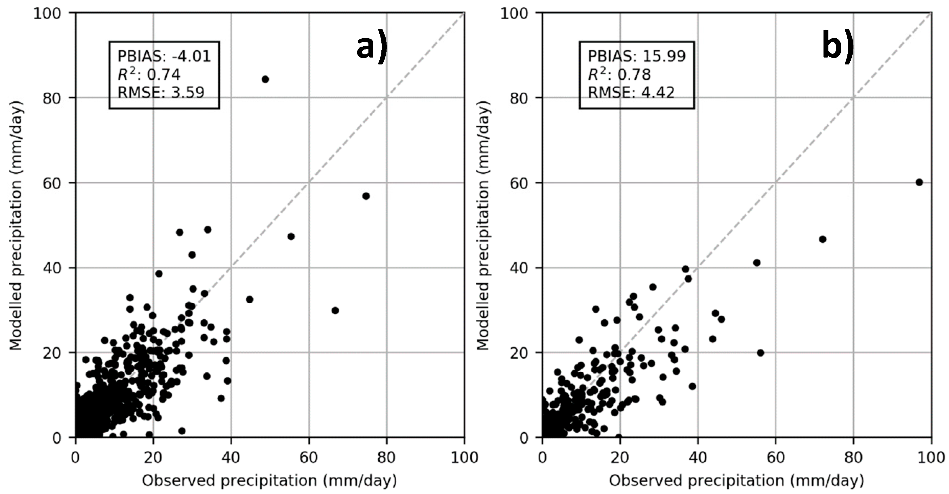
- Hénin, R.; Liberato, M.L.R.; Ramos, A.M.; Gouveia, C.M. Assessing the use of satellite-based estimates and high-resolution precipitation datasets for the study of extreme precipitation events over the Iberian Peninsula. Water 2018, 10, 1688. [Google Scholar] [CrossRef]


| Area (km2) | Reference Set-Up | Sensitivity Analysis | Model Calibration | |||
|---|---|---|---|---|---|---|
| Top Width (m) | Depth (m) | Top Width + 25% (m) | Depth + 100% (m) | Top Width (m) | Depth (m) | |
| 37.85 | 12.71 | 0.42 | 15.89 | 0.84 | 12.71 | 2.0 |
| 62.65 | 16.45 | 0.51 | 20.56 | 1.02 | 16.45 | 2.0 |
| 84.49 | 19.16 | 0.58 | 23.95 | 1.16 | 19.16 | 2.0 |
| 123.35 | 23.24 | 0.67 | 29.05 | 1.34 | 23.24 | 3.0 |
| 161.9 | 26.71 | 0.75 | 33.39 | 1.50 | 26.71 | 3.0 |
| 195.1 | 29.38 | 0.81 | 36.72 | 1.62 | 29.38 | 3.0 |
| 312.45 | 37.36 | 0.98 | 46.70 | 1.96 | 37.36 | 3.0 |
| 503.12 | 46.95 | 1.17 | 58.69 | 2.34 | 46.95 | 4.0 |
| 1164.36 | 73.16 | 1.65 | 91.45 | 3.30 | 73.16 | 4.0 |
| 2246.34 | 102.33 | 2.14 | 127.91 | 4.28 | 102.33 | 4.0 |
| 2785.08 | 114.21 | 2.33 | 142.76 | 4.66 | 114.21 | 4.0 |
| ID | θs | θr | η | Ksat,ver | α | l |
|---|---|---|---|---|---|---|
| 1 and 2 | 0.4912 | 0 | 1.9131 | 1.64 × 10⁻⁶ | 3.47 | −4.3 |
| 3 | 0.4646 | 0 | 1.116 | 2.26 × 10⁻⁵ | 12.84 | −5.0 |
| 4 | 0.4086 | 0 | 1.1335 | 5.05 × 10⁻⁶ | 7.00 | −5.0 |
| 5 | 0.4332 | 0 | 1.1701 | 9.93 × 10⁻⁷ | 3.36 | −5.0 |
| 6 | 0.4133 | 0 | 1.1191 | 1.43 × 10⁻⁶ | 2.27 | −5.0 |
| 7 and 8 | 0.3839 | 0 | 1.1206 | 4.29 × 10⁻⁶ | 7.17 | −5.0 |
| 9 | 0.4322 | 0 | 1.1701 | 9.93 × 10⁻⁷ | 3.36 | −5.0 |
| 10 | 0.4133 | 0 | 1.1191 | 1.43 × 10⁻⁶ | 2.27 | −5.0 |
| 11 and 12 | 0.3839 | 0 | 1.1206 | 4.29 × 10⁻⁶ | 7.17 | −5.0 |
| Depth (m) | Layers Thickness (m) | |||||||||||||
|---|---|---|---|---|---|---|---|---|---|---|---|---|---|---|
| 1st Horizon | 2nd Horizon | 3rd Horizon | ||||||||||||
| Reference Simulation | 5 | 0.3 | 0.3 | 0.7 | 0.7 | 1.5 | 1.5 | |||||||
| S7 | 5 | 0.15 | 0.15 | 0.15 | 0.15 | 0.35 | 0.35 | 0.35 | 0.35 | 0.75 | 0.75 | 0.75 | 0.75 | |
| S8 | 10 | 0.3 | 0.3 | 0.7 | 0.7 | 1.0 | 1.0 | 1.5 | 2.0 | 2.5 | ||||
| Simulation (% Variation) | Class (%) | ||||
|---|---|---|---|---|---|
| 0−10 | 10−40 | 40−60 | 60−90 | 90−100 | |
| Reference Simulation (m3 s−1) | 241.25 | 75.69 | 12.45 | 3.82 | 0.89 |
| 1 | −71 | −80 | −88 | −92 | −97 |
| 2 | +1 | +4 | +5 | +7 | +9 |
| 3 | +11 | −1 | +1 | +2 | +4 |
| 4 | +39 | −11 | +5 | +9 | +30 |
| 5 | −27 | +1 | +153 | +188 | +116 |
| 6 | −4 | +1 | +48 | +91 | +161 |
| 7 | +1 | +3 | −3 | −2 | −22 |
| 8 | −6 | 0 | +53 | +119 | +289 |
| 9 | +6 | +3 | +1 | 0 | 0 |
| 10 | −23 | −3 | +7 | +6 | +10 |
| 11 | −1 | +8 | +19 | +14 | −8 |
| 12 | −1 | +3 | +9 | +6 | −6 |
| 13 | 0 | 0 | 0 | 0 | 0 |
| 14 | +12 | +54 | +181 | +434 | +1531 |
| 15 | −37 | −57 | −63 | −71 | −85 |
| 16 | −69 | −87 | −87 | −90 | −97 |
| Simulation | Class (%) | ||||
|---|---|---|---|---|---|
| 0−10 | 10−40 | 40−60 | 60−90 | 90−100 | |
| 1 | 0.42 | 0.48 | 0.88 | 0.67 | 0.93 |
| 2 | 0.01 | 0.03 | 0.05 | 0.05 | 0.09 |
| 3 | 0.07 | 0.04 | 0.02 | 0.02 | 0.04 |
| 4 | 0.26 | 0.09 | 0.05 | 0.06 | 0.29 |
| 5 | 0.17 | 0.14 | 1.52 | 1.41 | 1.20 |
| 6 | 0.17 | 0.14 | 0.48 | 0.64 | 1.52 |
| 7 | 0.01 | 0.02 | 0.03 | 0.02 | 0.21 |
| 8 | 0.04 | 0.04 | 0.52 | 0.82 | 2.71 |
| 9 | 0.04 | 0.02 | 0.01 | 0.00 | 0.00 |
| 10 | 0.14 | 0.10 | 0.08 | 0.04 | 0.10 |
| 11 | 0.02 | 0.05 | 0.20 | 0.13 | 0.08 |
| 12 | 0.01 | 0.02 | 0.09 | 0.05 | 0.06 |
| 13 | 0.00 | 0.00 | 0.00 | 0.00 | 0.00 |
| 14 | 0.07 | 0.28 | 1.79 | 2.94 | 14.32 |
| 15 | 0.21 | 0.33 | 0.63 | 0.51 | 0.82 |
| 16 | 0.39 | 0.20 | 0.88 | 0.65 | 0.94 |
| Simulation | Computation Time (s day−1) | ||
|---|---|---|---|
| Minimum | Mean | Maximum | |
| Reference Simulation | 238 | 402 | 1764 |
| S1 | 29 | 83 | 550 |
| S2 | 190 | 319 | 2011 |
| S3 | 228 | 389 | 1513 |
| S4 | 255 | 399 | 1269 |
| S5 | 213 | 422 | 1947 |
| S6 | 237 | 407 | 1702 |
| S7 | 354 | 528 | 2829 |
| S8 | 303 | 447 | 2155 |
| S9 | 235 | 404 | 1752 |
| S10 | 234 | 399 | 1723 |
| S11 | 216 | 360 | 1711 |
| S12 | 221 | 359 | 1600 |
| S13 | 231 | 334 | 1599 |
| S14 | 209 | 309 | 1437 |
| S15 | 6 | 65 | 475 |
| S16 | 5 | 52 | 448 |
| Station | Calibration | Validation | ||||||
|---|---|---|---|---|---|---|---|---|
| R2 (-) | RSR (-) | PBIAS (%) | NSE (-) | R2 (-) | RSR (-) | PBIAS (%) | NSE (-) | |
| Sar | 0.75 | 0.53 | 0.18 | 0.72 | 0.83 | 0.44 | 16.09 | 0.81 |
| Ulla | 0.56 | 0.67 | −11.24 | 0.55 | 0.76 | 0.53 | −18.54 | 0.72 |
| Arnego-Ulla | 0.70 | 0.55 | −12.29 | 0.69 | 0.78 | 0.49 | −16.82 | 0.76 |
| Deza | 0.74 | 0.53 | −8.96 | 0.72 | 0.85 | 0.40 | −4.35 | 0.84 |
Publisher’s Note: MDPI stays neutral with regard to jurisdictional claims in published maps and institutional affiliations. |
© 2020 by the authors. Licensee MDPI, Basel, Switzerland. This article is an open access article distributed under the terms and conditions of the Creative Commons Attribution (CC BY) license (http://creativecommons.org/licenses/by/4.0/).
Share and Cite
Oliveira, A.R.; Ramos, T.B.; Simionesei, L.; Pinto, L.; Neves, R. Sensitivity Analysis of the MOHID-Land Hydrological Model: A Case Study of the Ulla River Basin. Water 2020, 12, 3258. https://doi.org/10.3390/w12113258
Oliveira AR, Ramos TB, Simionesei L, Pinto L, Neves R. Sensitivity Analysis of the MOHID-Land Hydrological Model: A Case Study of the Ulla River Basin. Water. 2020; 12(11):3258. https://doi.org/10.3390/w12113258
Chicago/Turabian StyleOliveira, Ana R., Tiago B. Ramos, Lucian Simionesei, Lígia Pinto, and Ramiro Neves. 2020. "Sensitivity Analysis of the MOHID-Land Hydrological Model: A Case Study of the Ulla River Basin" Water 12, no. 11: 3258. https://doi.org/10.3390/w12113258
APA StyleOliveira, A. R., Ramos, T. B., Simionesei, L., Pinto, L., & Neves, R. (2020). Sensitivity Analysis of the MOHID-Land Hydrological Model: A Case Study of the Ulla River Basin. Water, 12(11), 3258. https://doi.org/10.3390/w12113258