Article

Impact of Jetty Configuration Changes on the Hydrodynamics of the Subtropical Patos Lagoon Estuary, Brazil

by
Maria Helena Paulo António
1,2,*,
Elisa H. Fernandes
1 and
Jose H Muelbert
3
1
Laboratório de Oceanografia Costeira e Estuarina, Instituto de Oceanografia, Universidade Federal do Rio Grande, CP 474, Rio Grande CEP 96201-900, Brazil
2
Escola Superior de Ciências Marinhas e Costeiras, Universidade Eduardo Mondlane, Quelimane 128, Mozambique
3
Laboratório de Ecologia do Ictioplâncton, Instituto de Oceanografia, Universidade Federal do Rio Grande, CP 474, Rio Grande CEP 96201-900, Brazil
*
Author to whom correspondence should be addressed.
Water 2020, 12(11), 3197; https://doi.org/10.3390/w12113197
Submission received: 16 September 2020 / Revised: 23 October 2020 / Accepted: 5 November 2020 / Published: 16 November 2020

Abstract

:
Coastal infrastructure alterations, such as jetty expansions, are designed to provide improvements to natural dredging and safety of marine access and to maximize the management and efficiency of ports. Furthermore, these alterations have the potential to cause significant environmental changes to estuaries and adjacent coastal areas. Here, the hydrodynamics of Pathos Lagoon was investigated before and after the jetty alterations, where the jetty was increased by approximately 10–18% and the mouth width was reduced by 15%. The TELEMAC-3D numerical model was calibrated and validated using the field data, and then simulated for characteristic low and high extreme discharge years for the old and new jetty configurations. Results showed a flow reduction of approximately 20% both in the ebb and flood conditions in the new configuration, which was accompanied by a slight change in the propagation angle of the western jetty current. Reduction of the saltwater intrusion was registered during both the high and low discharge conditions with the new jetty configuration. During the high discharge periods with NE winds, saltwater intrusion did not reach the previous estuarine inland boundary. During the period of low discharge with SW wind, salinity did not reach further than 180 km inland. Reduced saltwater intrusion was estimated landwards and in the shallow embayments. The horizontal stratification structure of the salinity changed, with the partial centralization of the flow in the access channel. The observed hydrodynamic changes from the infrastructure modifications could affect the estuarine ecosystem by increasing the sediment retention, reducing the transport of marine organisms and water properties into the estuary. This study contributes not only to the understanding of hydrodynamic changes but also to the potential optimization of estuarine and coastal management strategies.

Graphical Abstract

1. Introduction

Approximately 60% of the world’s population inhabits coastal regions [1], and most of it is located around estuarine areas. Important ports and large cities are located inside estuaries, making them vulnerable to changes by natural processes and anthropogenic alterations associated with economic development [2,3]. Changes in the geomorphology, river discharge, and circulation patterns influence pollution and the distribution of nutrients and suspended sediments [2]. The ecological consequence of these alterations is enhanced because estuaries serve as habitats and nurseries for the initial stages of the development of many species [4,5], are rich in nutrients, influence primary production [6], and provide abundant food and protection against predators [7,8].
Studies on human-induced impacts on the hydrodynamics, saltwater intrusion, sediment transport, pollutant dispersion, and ecology of coastal systems have been gaining ground during the last century. Port expansions can increase sedimentation and the migration of tidal delta and infill of channels [2]. Jetty construction can change the direction of the tidally induced currents, influence the evolution of the bed level, and induce sedimentation and erosion [9]. It can also reduce the wave height and flushing rates and increase sedimentation and pollution [10]. It has also been reported that the extension of jetties does not change inlet flow propagation and water quality, although changes in the topography increase current velocities and salinity values [11]. Dredging activities can cause variations in the estuarine physical parameters and suspended sediment concentration; moreover, they can promote fast siltation in the harbor waterway after the end of the dredging operations [12].
The Port of Rio Grande, which is located in the Patos Lagoon estuary (Figure 1) in the southernmost part of Brazil, is the third-largest port in Brazil [13]. To respond to the commercial demands for port expansion, human intervention has been necessary since the last century to ensure safety and navigation conditions. The first alteration to the access channel was the construction of two approximately 3 km long jetties at the mouth of the Patos Lagoon in 1907 [14]. In 2010, adjustments in the original project were carried out, and the jetties were lengthened by 370 m (east) and 700 m (west). This alteration aimed to improve navigation conditions by allowing a progressively deeper channel, which reached a depth of 16 m inside and 18 m outside of the estuarine access channel, and by reducing the width of the estuary mouth. The concept behind this last modification was to converge the jetties at the mouth to increase the flood velocities and promote natural dredging [15].
Patos Lagoon is the largest choked coastal lagoon in the world [16] and extends 250 km with a 40 km width and a total area of 10,360 km2 (Figure 1). The lagoon connects to the Atlantic Ocean through a 700 m wide channel. The southern estuarine portion of the lagoon represents 10% of the total area and has an average depth of 5 m [17] and natural and dredged channels of up to 16 m [18]. The estuary is microtidal, and its dynamics is controlled by wind action and freshwater discharge [15,19,20]. Tides are mixed with diurnal predominance, and with an amplitude of approximately 0.23 m [21], which is restricted to the coast and the lower estuary [22] and contributes to the mixing of the water column and the landward water transport [23,24]. The freshwater discharge is typical of that in the temperate regions, with a historical annual mean runoff of approximately 2400 m3 s−1. ENSO (El Niño-Southern Oscillation) variability plays an important role in changing the river flow behavior, with high discharge values of approximately 12,000 m3 s−1 during El Niño years and low values of 500 m3 s−1 during La Niña [18].
Most studies on the hydrodynamics of the Patos Lagoon estuary were carried out before 2010 [17,23,25] or were based on the old access channel configuration [26,27]. Only a few studies focused on the environmental consequences of the jetty modernization, which was concluded in 2010. In [14], the authors investigated changes in the fine sediment dynamics in the access channel of Patos Lagoon and indicated that changes in the deposition pattern and the redistribution at the bottom occurred due to the new configuration. In [15], the authors concluded that the access channel modification resulted in changes in the erosion and deposition rates and the longitudinal growth of the sand spits. However, investigations of the hydrodynamic characteristics after the modernization of the jetties have not yet been conducted.
This study investigated changes in the hydrodynamics of Patos Lagoon after the alteration concluded in 2010. A three-dimensional numerical model was used to test the hypothesis that even small infrastructure alterations in coastal environments can lead to hydrodynamic changes. If proven correct, these changes could lead to alterations in the flow pattern and modification of the saltwater intrusion, stratification, and mixing characteristics that could have potential environmental consequences.

2. Numerical Model

This study was carried out with the TELEMAC-3D model [28] to simulate the hydrodynamics of the Patos Lagoon system with the old and new jetty configurations of the lagoon access channel. The model was run with high and low freshwater discharge conditions, which coincided with the El Niño (2002 to 2003) and La Niña (2011 to 2012) simulated periods (Figure 2).

2.1. Model Description
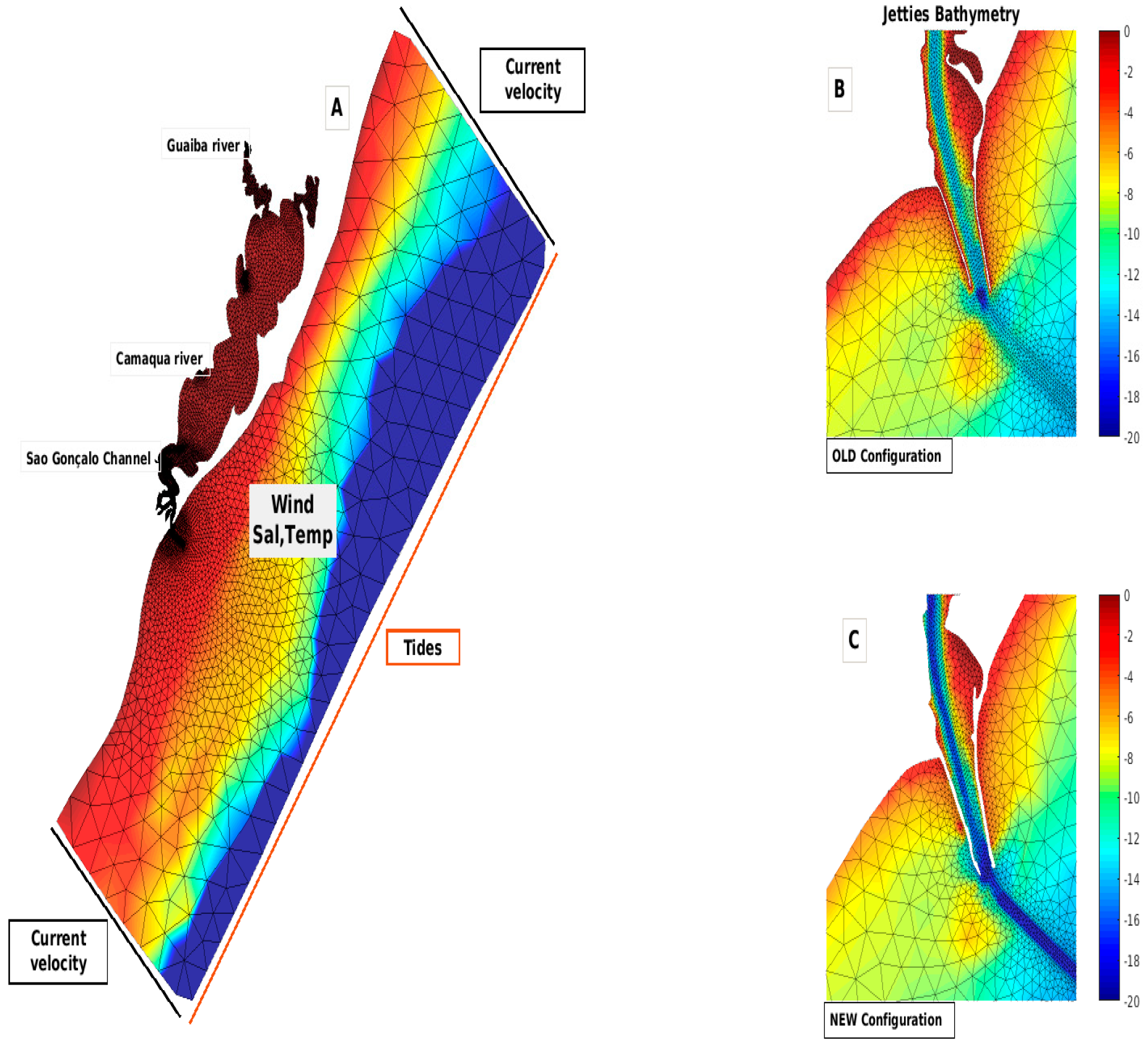
The TELEMAC-MASCARET model (V7P0 version, Laboratoire National d’Hydraulique et Environnement of the Company Electricité of France (©EDF): Paris, France.) presents modules in two and three dimensions to study the hydrodynamics, sediment transport, waves and water quality of coastal and oceanic regions. The hydrodynamic model solves the Reynolds-averaged Navier–Stokes equations and considers the local variations in the free surface of the fluid, neglecting the variation of density in the mass conservation equation, offering the choice of considering the hydrostatic or non-hydrostatic pressure and applying the Boussinesq approximation to solve the motion equation. In this study, simulations were carried out in the hydrostatic mode. This model applies the finite element method to solve the hydrodynamic equations and uses the sigma coordinate system for vertical discretization. Its domain is discretized by a non-structured grid of finite elements (triangular elements), which allows the concentration of a higher number of elements in regions of interest and/or significant bathymetric variations and lower resolutions in regions of more homogeneous bathymetry, which reduces computational time. Details of the model formulations were presented by [29].

2.2. Model Grid

The bathymetry of Patos Lagoon, the estuary, and the adjacent coastal region was obtained from historical data. Nautical charts from the Directory of Hydrography and Navigation (DHN, Brazilian Navy) for before 2010 were used as the “old” bathymetric information (before changes in configuration). Data from the jetty expansion project were used to define the bathymetry after the alteration of the jetties. The main difference between the two grids was the length of the jetties and the depth of the access channel to the estuary (Figure 3). The BlueKenue Software (https://nrc.canada.ca/en/research-development/products-services/software-applications/blue-kenuetm-software-tool-hydraulic-modellers) was used to generate the unstructured bathymetric grids of the triangular elements. Grid optimization was conducted on the complex morphology and the shallow areas inside the estuary and in the adjacent coastal regions, which allowed higher resolution in the regions of interest (Figure 3).
Two resulting grids were used to reproduce the hydrodynamics before and after the modification of the jetties (Figure 3B,C). The grids encompassed the entire study area up to approximately 2500 m depth to better represent the coastal dynamics. The generated grids contained a total of 17,868 and 17,575 node points for the old and new scenarios, respectively. The largest triangles located in the open sea (lowest refinement) had edges of approximately 27 km in length, while the smallest triangles in the access channel (highest refinement) were approximately 50 m.

2.3. Initial and Boundary Conditions

The open boundaries of the domain were run with the results from regional and global models and field data (Figure 3). To ensure comparability, simulations for both scenarios used the same settings. The altimeter sea level and velocity data were obtained from the TPXO Project (internally coupled to the TELEMAC model) and were used to set up the conditions at the oceanic boundary. Time series of the daily averaged river discharges of the main tributaries (Guaíba River and Camaquã River) were obtained from the National Water Agency [30] and prescribed for the northern and central continental boundaries. The mean discharge data for São Gonçalo Channel was considered constant at 700 m3 s−1 [31] due to the lack of available data for the studied periods. Temperature and salinity fields obtained from the HYCOM model (Hybrid Model Coordinate Oceanic, [32]), with a temporal resolution of 3 h and a spatial resolution of 1/12.5°, were prescribed tridimensionally for all grid points. Wind time series data with spatial and temporal resolutions of 0.75° and 6 h, respectively, were obtained from the ECMWF (European Center for Medium-Range Weather Forecasts, [33]).
Eleven (11) sigma levels were considered in the vertical direction and were distributed from the bottom to the sea surface.

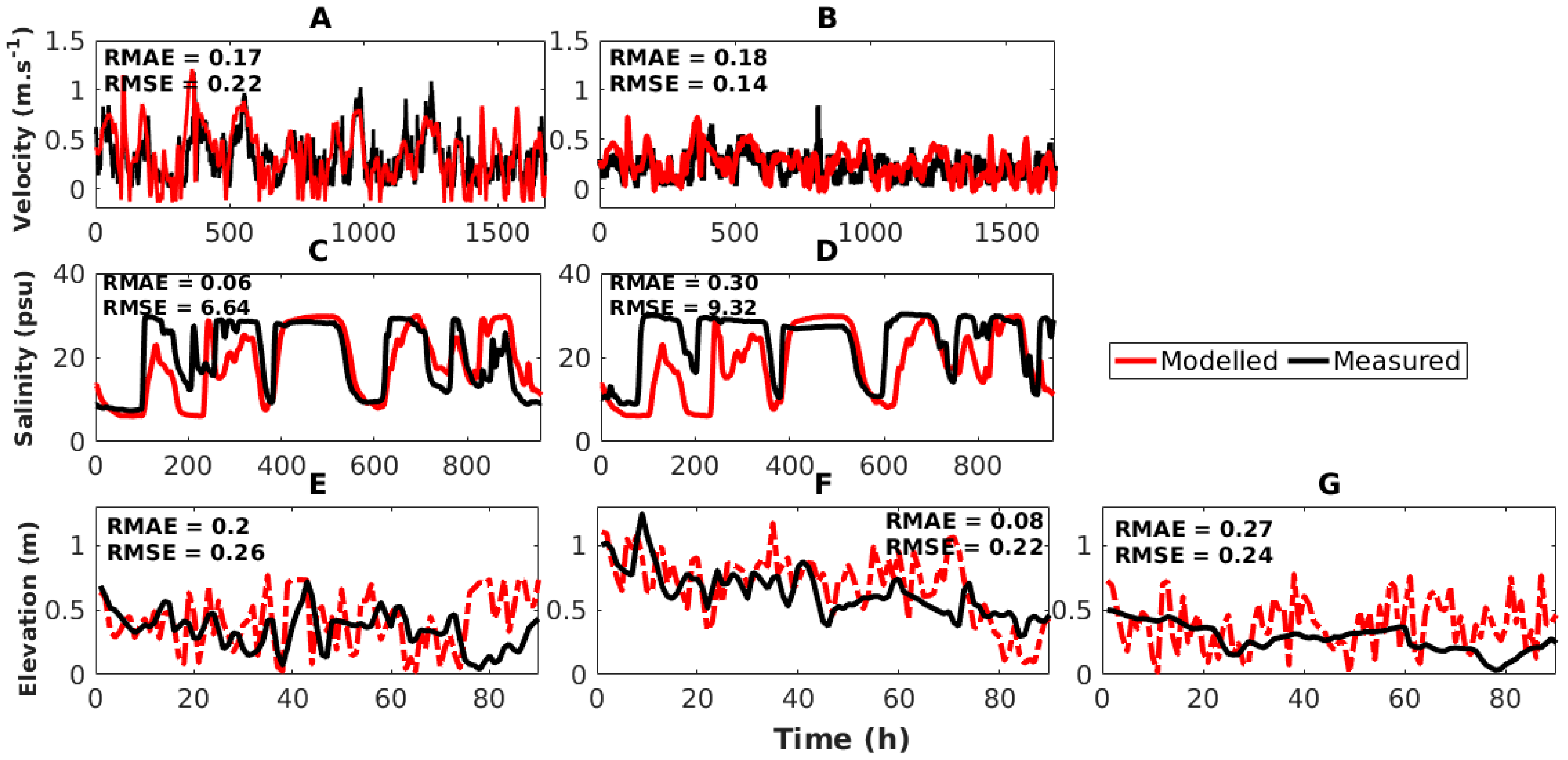
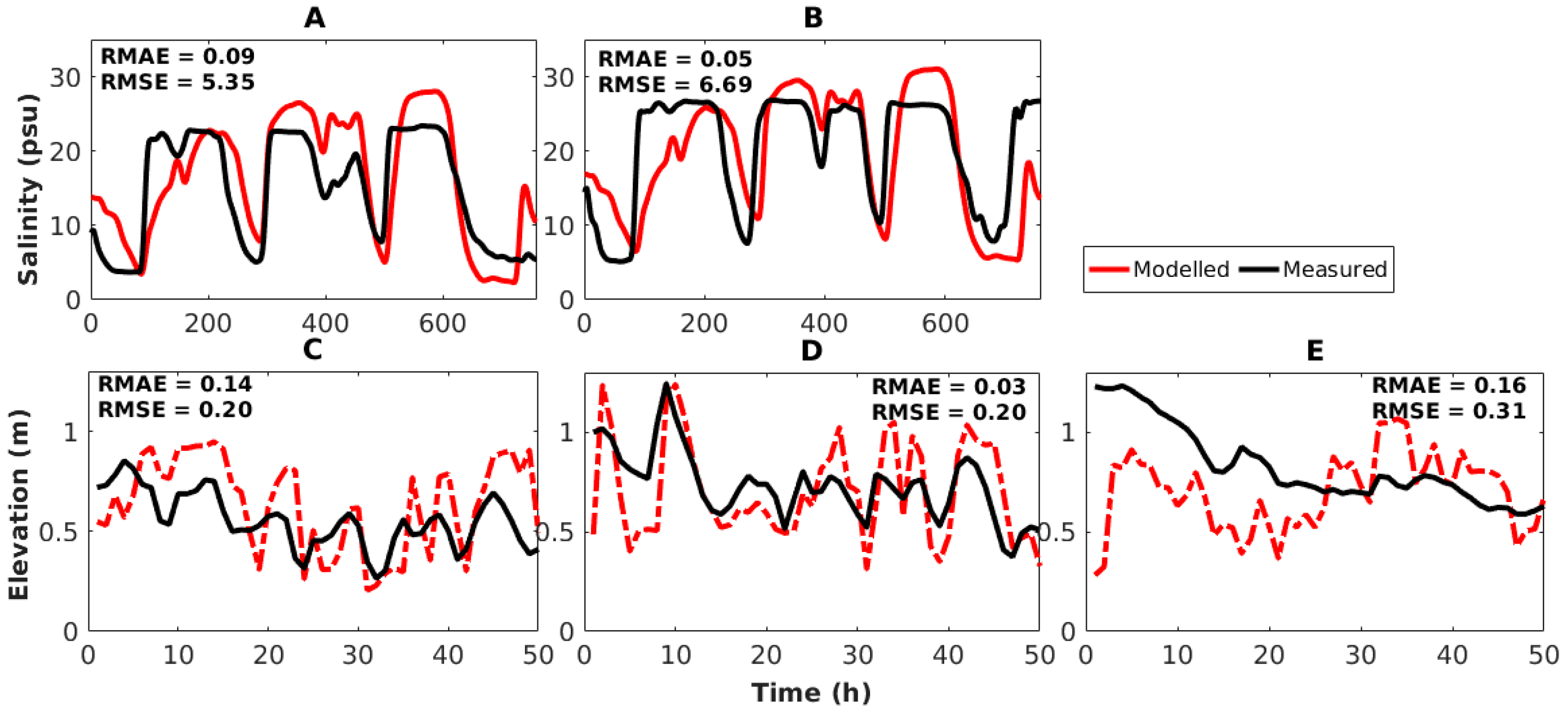
2.4. Calibration and Validation
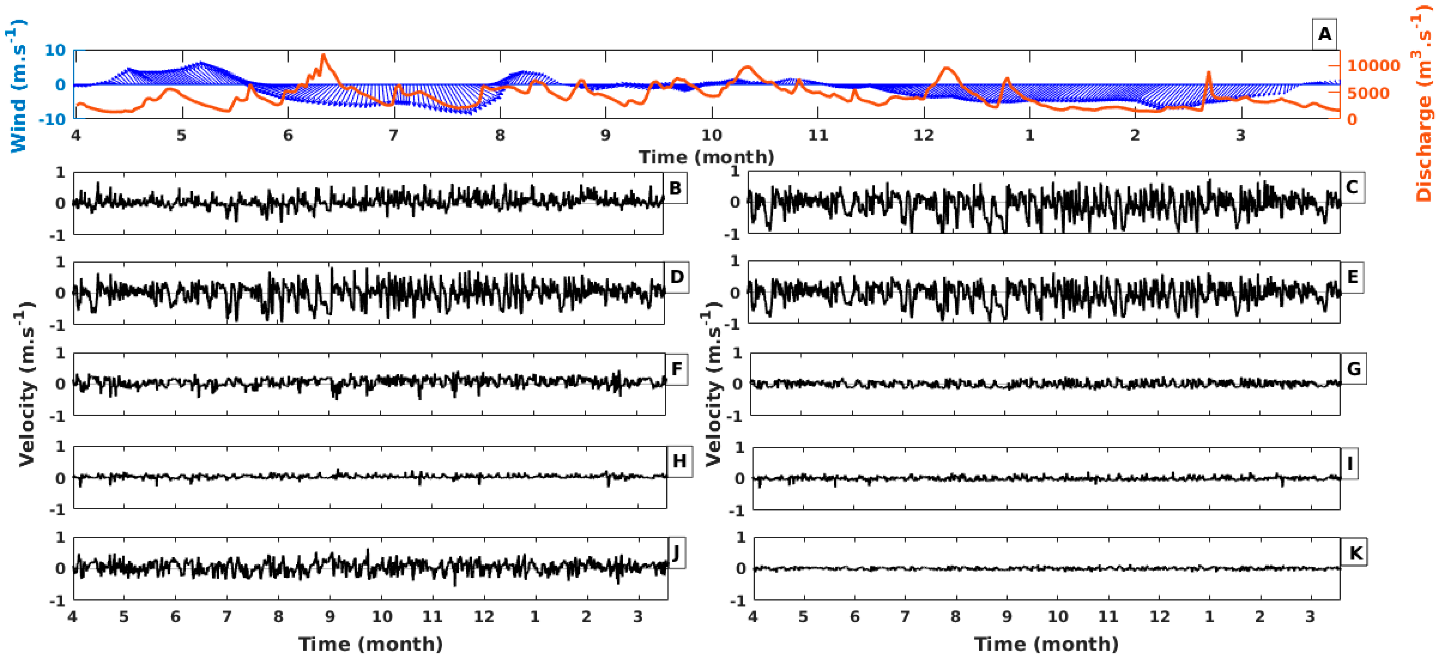
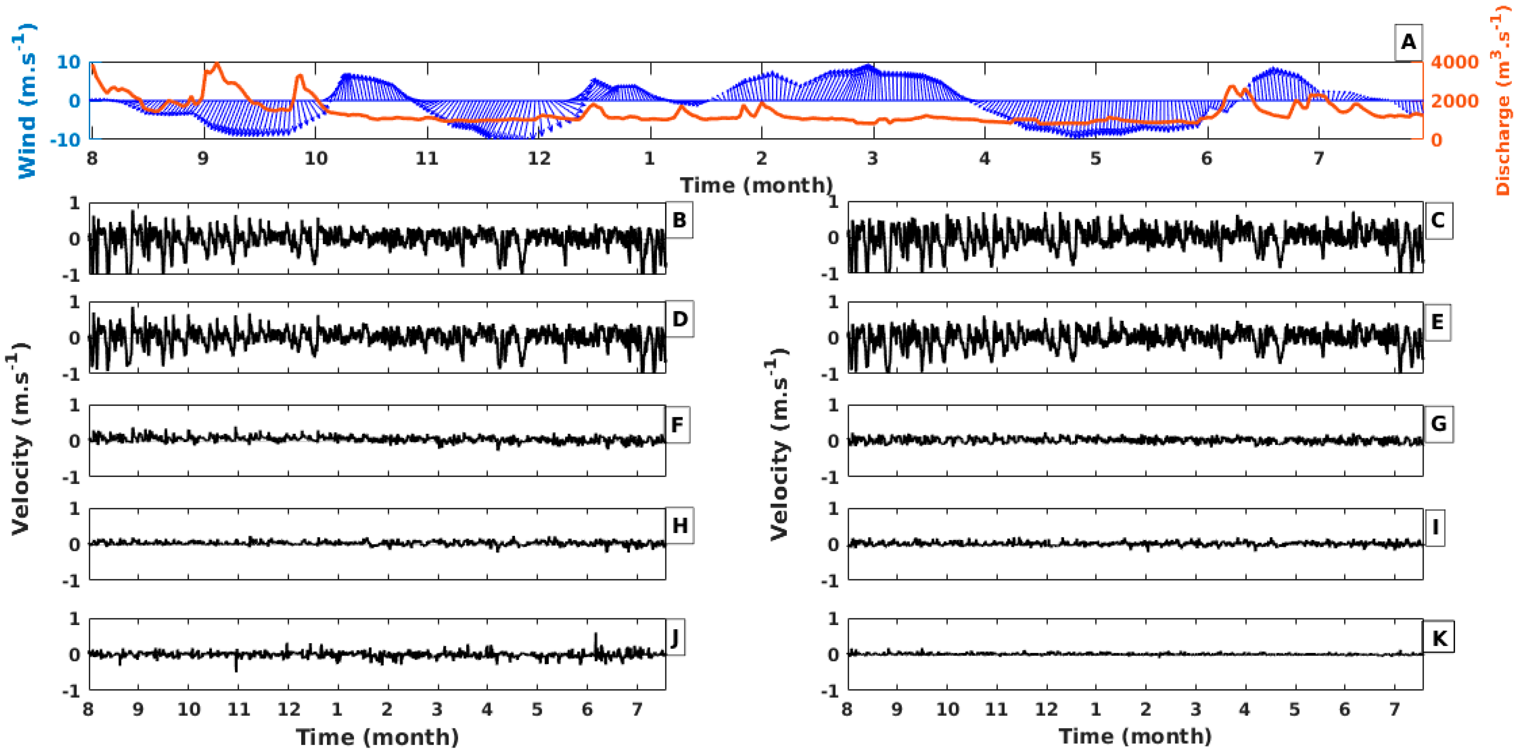
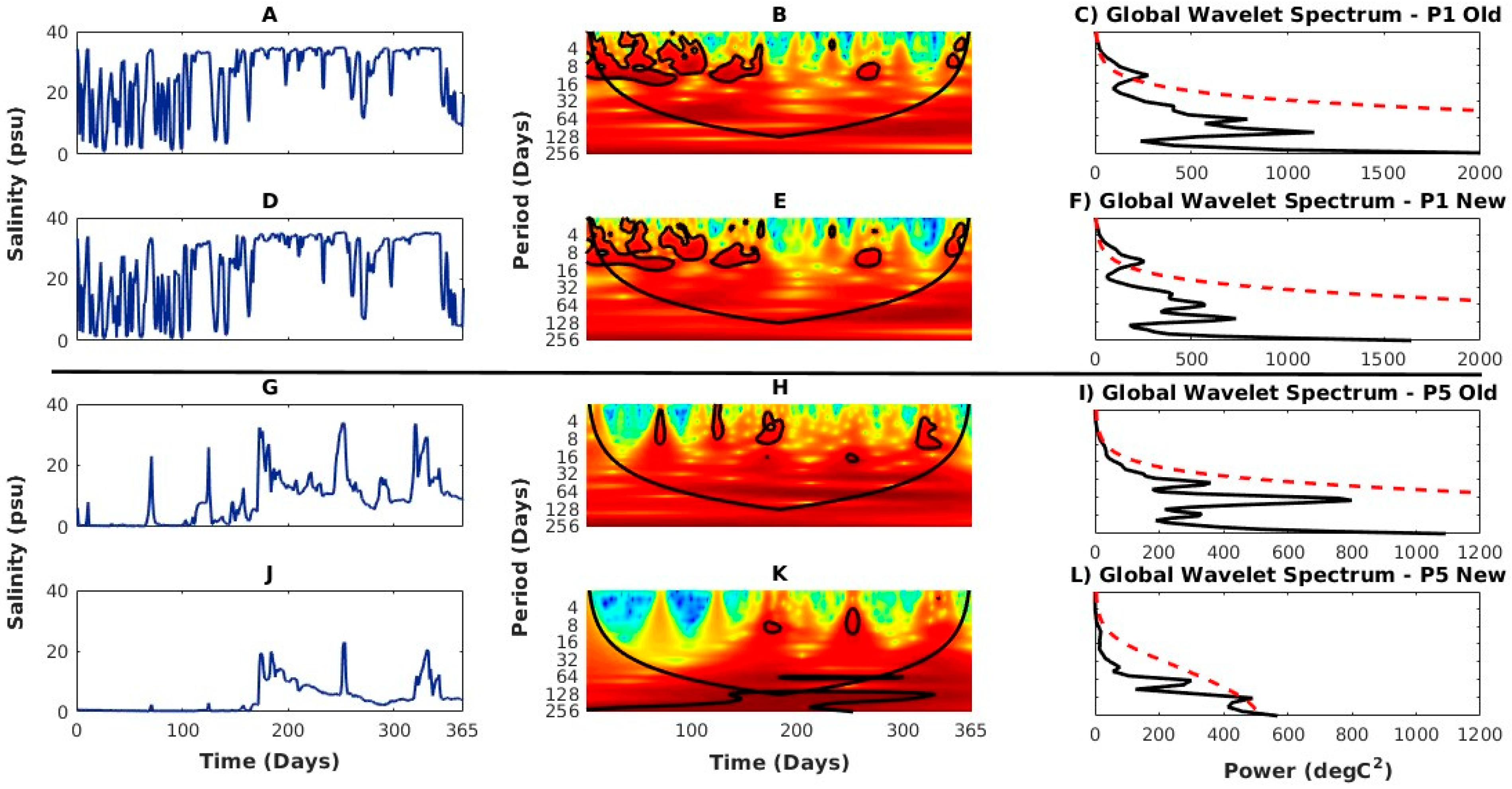
Previous studies [19,26,34] using TELEMAC in Patos Lagoon performed calibration and validation exercises to demonstrate the ability of the model to reproduce the observed environmental conditions. In the present study, calibration tests were carried out for both scenarios with the same initial and boundary conditions settings. The tests were conducted with the main physical parameters (Supplementary Table S1), and the best model reproduction was obtained with Smagorinsk = 10−6 as the horizontal turbulent model, mixing length (Prandtl) = 10−6 as the vertical turbulent model, Manning = 0.03 as law of bottom friction, the Coriolis constant = −7.7 × 10⁻⁵ Nm−1 s−1 and the wind influence coefficient = 1 × 10⁻⁵ Nm−1 s−1 for the old and 5 × 10⁻⁵ Nm−1 s−1 for the new jetty configuration during both simulation periods. The simulations were performed for October to November 2006 for the old configuration and for October to November 2010 for the new configuration (Figure 3). The model performance was evaluated by comparing the modeled and measured current velocities using the root mean square error (RMSE) and the relative mean absolute error (RMAE) [31]. The model performance was classified as excellent when values of RMAE were smaller than 0.2; good, when values were between 0.2 and 0.4; reasonable, when values were between 0.4 and 0.7; poor, when values were between 0.7 and 1; and bad, when values were greater than 1 [35]. The model calibration tests for both scenarios resulted in model performances ranging from good to excellent for the current velocity time series at the surface (old RMAE = 0.31 and new RMAE = 0.07) and bottom (old RMAE = 0.27 and new RMAE = 0.01) (Figure 4).
The TELEMAC model validation was also carried out for both scenarios with the same initial and boundary condition settings for both simulations and considered the same set of physical parameters that generated the best model performance in the calibration tests. Salinity, water elevation and current velocity modeling results were compared with field data for the period between October and November 2006 for the old jetty configuration (Figure 5) and October to November 2010 for the new configuration (Figure 6). The model validation tests for both scenarios resulted in model performances ranging from good to excellent (Table 1).

2.5. Data Analysis

To analyze the effect of alterations in the Patos Lagoon estuary access channel on the hydrodynamics and saltwater intrusion, the difference between the current velocity and salinity fields, respectively, in the two configurations were calculated and analyzed in terms of continental discharge and wind (direction and intensity) variability. The time series of current velocity and salinity were also extracted from the model results for points P1, P2, P3, P4 and P5 during the high discharge simulations and P1, P2, P3, P4, P5, P6, P7 and P8 during the low discharge simulations at the surface and bottom (Figure 1). Salinity fields of representative time steps were chosen for the periods of high and low discharge during the maximum flood and ebb conditions.
The time scale of the wind effect on the saltwater behavior into the estuary during high and low discharge was investigated. The spectral contents and the correlations between the daily time series of salinity were carried out using Morlet wavelet analysis [36] at points P1, P2, P3, P4 and P5 and P1, P2, P3, P4, P5, P6, P7, and P8. A background Fourier red noise spectrum (α = 0.72) was assumed at each scale, and then the chi-squared distribution was used to find the 95% confidence (5% significance) contour.
To investigate changes in the lateral and vertical stratification between the jetty configurations, profiles of salinity were extracted during the periods of lateral ebb and flood. The spatial differences between the old and new configurations were calculated. In addition, changes in the intensity and incidence angle of the current velocities between the jetties were investigated.

3. Results

The numerical simulations considering the new and old jetty configurations at the mouth of the Patos Lagoon estuary in periods of high and low continental discharge were analyzed comparatively. The high discharge simulation (El-Niño 2002–2003) was marked by an average discharge of 4200 m3 s−1, with a maximum of 12,300 m3 s−1 during mid-June 2002 and a minimum of 1336 m3 s−1 during February 2003. The predominant wind was from the north, with the NE winds reaching a maximum intensity of approximately 8 m s−1. During the low discharge simulation (La Niña 2011–2012), the minimum discharge was approximately 806 m3 s−1 for several months, with an average of 1370 m3 s−1 and a maximum of 4000 m3 s−1. The winds were mainly from the north and south quadrants, with the NE and SW wind intensities close to 10 m s−1 (Figure 7).

3.1. Hydrodynamics

To analyze the effects of the access channel modifications on the dynamics of the Patos Lagoon estuary, current velocity time series at the surface and bottom were extracted from the modeling results for both the old and new jetty configurations. The model results were obtained for several points from the access channel landwards for the low and high discharge conditions (Figure 1). The difference between the current velocities of the old and new jetty configurations was calculated and analyzed as a function of discharge and wind direction and intensity.

3.1.1. High Discharge Simulation

The predominant winds during the simulated period were from the NE, and the mean river discharge was approximately 4200 m3 s−1, with peaks of 10,000 m3 s−1 (P1, Figure 7A).
The differences in the current velocity between the old and new configurations were higher at the bottom than at the surface and generally decreased landwards (Figure 7). The exception was at the estuarine limit (P5, Figure 1), where the difference increased at the surface (Figure 7J). The maximum difference in flood velocities was approximately 1 m s−1 at the entrance of the estuary (P1 and P2, Figure 7C,E). At the estuarine limit (P5, Figure 7J,K), however, differences at the surface were approximately 0.5 m s−1, while those at the bottom were almost nonexistent. Overall, the reduction in current velocity between the old and new configurations ranged from 10% to 20% at the surface and up to 50% at the bottom, mainly in the estuarine mouth region.

3.1.2. Low Discharge Simulations

During the simulated period, the wind pattern alternated between the NE and SW directions, and the river discharge varied from approximately 1370 m3 s−1 to 4000 m3 s−1.
Differences in current velocity between the old and new configurations were higher at the bottom than at the surface near the estuary entrance and decreased landwards (Figure 8). The difference in the ebb flow values between the old and new configurations was highest at the bottom, with a value of approximately −1.1 m s−1 at the estuarine entrance (P1 and P2, Figure 8C,E), and reached approximately 0.2 m s−1 at the surface and was almost null at the bottom in the estuarine limit (P5, Figure 8J,K). The reduction in the current velocity between the old and new configuration was similar to the reduction estimated in the high discharge simulation, with a reduction between 10% to 20% at the surface and up to 50% at the bottom at the estuary mouth. The analysis of additional points inside the Patos Lagoon revealed that differences in current velocity between the old and new configurations were more pronounced in the interior of the lagoon (P8, Supplementary Figure S1). The reduction in the current velocity from the old to the new configuration was similar in the other points at the surface (10%) and bottom (20%) (P6 and P7, Supplementary Figure S1).
At point P8 (Figure 1), the difference in current velocities between the two configurations was higher at the surface, with twice the difference of the other points, where the range was −1 to 0.5 ms−1, and the difference in the ebb flow was more than 50%.

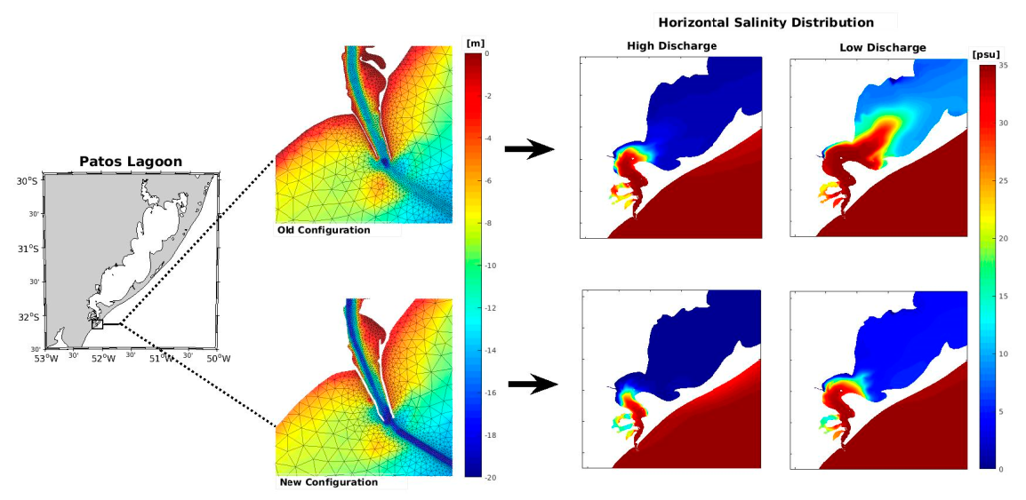
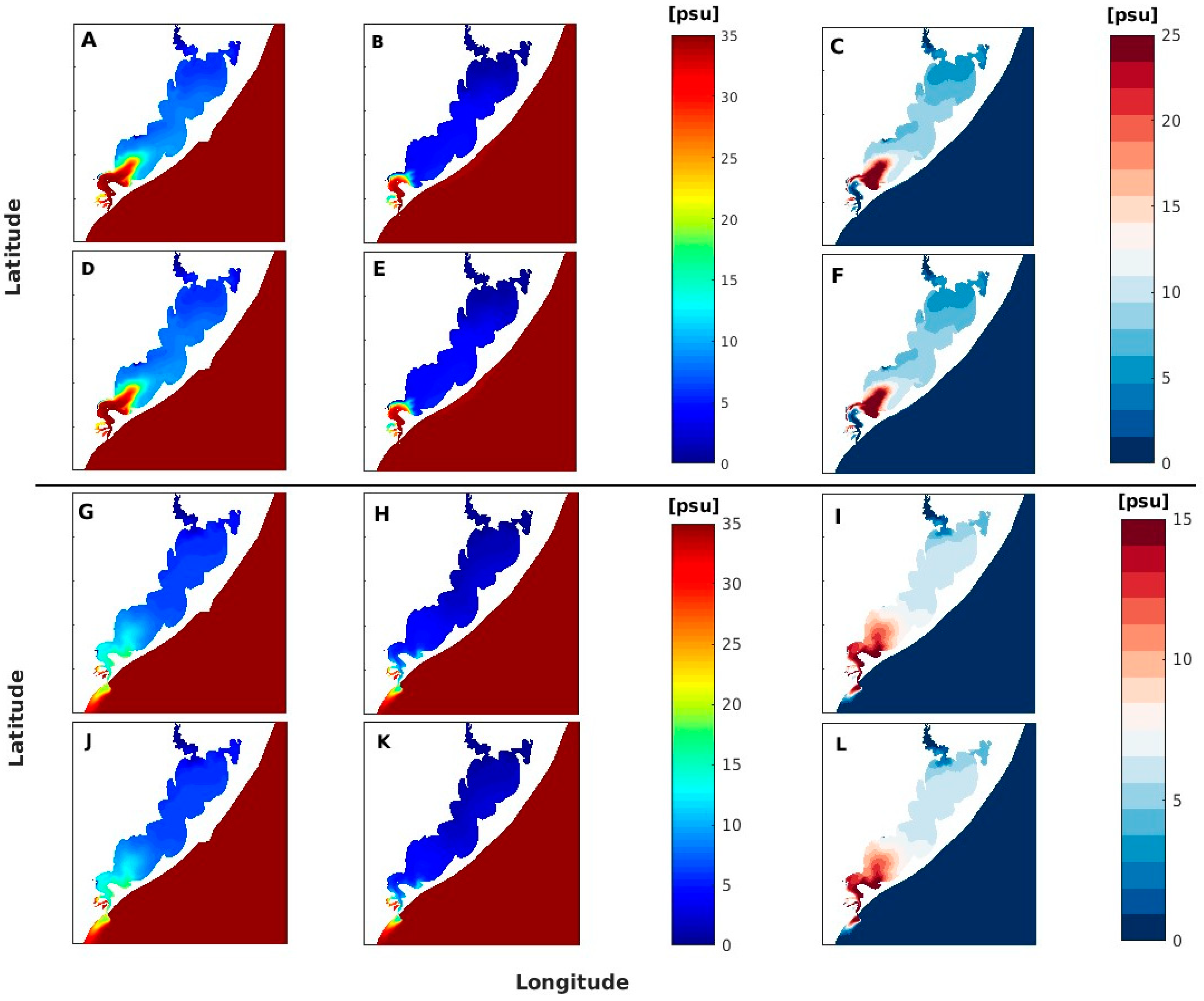
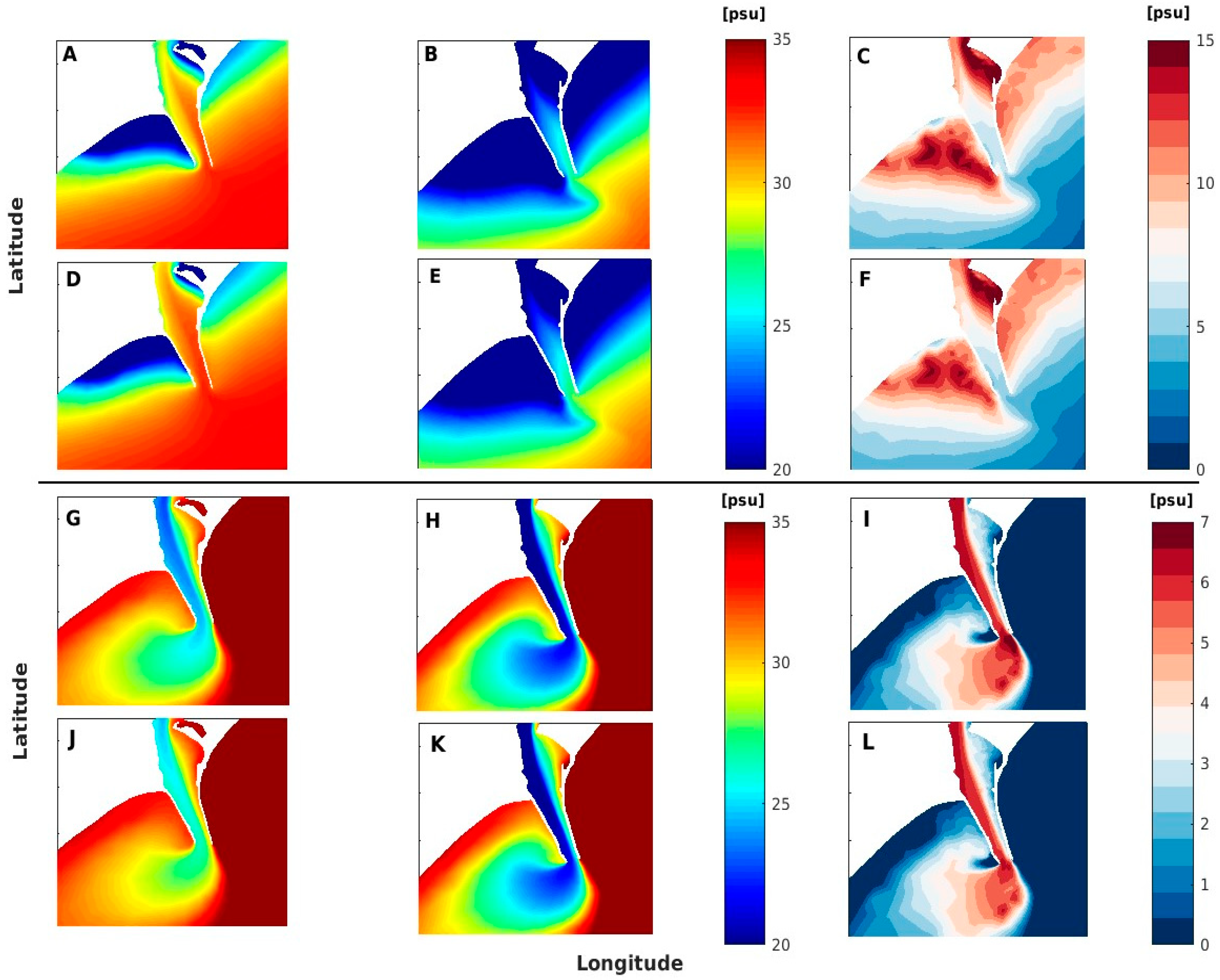
3.2. Alterations in Saltwater Distribution

3.2.1. High Discharge Simulation

Salinity behavior throughout both simulations (old and new scenarios) responded to the wind and freshwater discharge. Differences in salinity between the scenarios indicated that the saltwater excursion throughout the estuary decreased after the jetty alterations during the simulated period, with differences ranging from a few units to almost 25 units of salinity. The largest differences were estimated near the estuarine limit (P5, Figure 9J,K) at the surface and bottom. These results highlighted that the sporadic events of salinity intrusion towards the estuarine limit were reduced with the new jetty configuration (P5, Figure 9J,K).
Differences in salinity between the old and new jetty configurations ranged from 10 to 25 units in the shallow embayments and close to the estuarine boundary (Figure 10).
During flood conditions, salinity was reduced in more than 30% in the estuarine region with the new configuration (Figure 10C,F). During ebb conditions, a salinity reduction of up to 5 units was verified in the shallow embayments.
The variability in salinity presented a significant periodicity of approximately 10–15 days, with a similar response for both the old (Figure 11A–C) and new scenarios (Figure 11D–F) at the estuary entrance. The global power spectrum showed that only the frequencies at time scales <15 days were significant for the old and new configurations (Figure 11C,F). Results for the middle estuary (P4, Figure 11I,L), indicated that this periodicity of <15 days existed only during the first period of the simulation (April–June, August). The upper limit of the estuary (P5) presented a similar behavior (not shown). The signal of salinity intrusion lost strength towards the interior of the lagoon, and this decrease in energy was most evident with the new jetty configuration. A power value of 2500 C2 in the overall power at 15 days was estimated at the entrance of the estuary for both the old and new configurations (Figure 11C,F), but the interior of the estuary experienced a reduction from 1250 C2 to 300 C2 from the old (Figure 11I) to the new (Figure 11L) configuration.

3.2.2. Low Discharge Simulation

Similar to the behavior in the high discharge simulation, the salinity behavior during the low discharge simulations for the old and new scenarios were influenced by the wind and freshwater discharge. An increase in salinity was estimated in the Patos Lagoon under the continued predominance of S and SW winds and low discharge. The maximum salinity was estimated close to the estuarine mouth (P1, Figure 12) from mid-December to March. The maximum salinity was verified at point P3 (Figure 12F,G) after January and at point P5 (Figure 12J,K) at the end of April as a response to the saltwater intrusion from the ocean to the inner lagoon (approximately 250 km). This response lasted until the end of June and reached the northern region of the lagoon (P8, Supplementary Figure S2), even during the period from April to May, when the wind changed to the NE. In contrast to the old scenario, in the new jetty configuration, salinity values greater than 20 seldom reached the estuary limit. At approximately 120 km from the estuary mouth, a salinity increase was registered in mid-January with the old configuration but only increased in April with the new configuration (P6, where the edge effect become important (C, F, I and L) (the global wavelet power spectrum of the time series and the dotted red line indicate the 95% confidence level), and P7, Supplementary Figure S2M–P). With the old configuration, saltwater reached the mouth of Guaíba River, but was never recorded in the new scenario (P8, Supplementary Figure S2Q,R).
The lagoon was less saline in the new than in the old scenario at all points in both the surface and the bottom. The differences in salinity between both scenarios ranged from a few units to just over 20 units. Large differences in salinity were estimated at the surface and the bottom near the estuarine limit after the incidence of the increased saltwater intrusion due to the southerly winds from February to July. The sporadic salinity events that were registered with the old configuration were not verified with the new configuration (P4 and P5, Figure 12H–K). Results for Patos Lagoon revealed that salinity differences of up to 10 units can propagate to the northern limit of the lagoon (approximately 250 km from the estuary mouth) (Supplementary Figure S2). Differences in salinity decreased towards the northern end of the lagoon, from 10 at point P6 at the bottom (Supplementary Figure S2N) to less than 5 at Guaíba River mouth (Supplementary Figure S2Q,R).
The simulations with low river discharge revealed an increased difference in salinity between the old and the new jetty configuration (Figure 13). During the flood conditions, the salinity differences were the strongest, and decreased to approximately 25 in the southern lagoon, surpassing the northern limit of the estuary, and decreasing towards the interior of the lagoon to approximately 5 at Guaíba River mouth, both at the surface and bottom (Figure 13C,F,I,L). Differences in salinity of approximately 20 were evident inside the shallow estuarine embayments. During the ebb conditions, the lagoon also became less saline with the new jetty configuration than with the old configuration. Differences in salinity of approximately 10 were evident in the coastal regions and the shallow embayments close to the estuary mouth, while from the estuary limit to the north of the lagoon, the difference did not exceed 5 units (Figure 13I,L) and had the same spatial dimension as during the flood period.
Similar to the high discharge results, during low river discharge conditions, salinity presented a periodicity of approximately 10–15 days for both the old and new jetty configurations (Figure 14A–F) at P1 to P3 (not shown). Results of the global power spectrum analysis highlighted that the time scale frequencies <15 days were significant for the old and new configurations (Figure 14C,F). Results indicated significant salinity variability in the first 150 days of the simulation in the southern lagoon region (P1, P2, and P3, Figure 1) during August–September and November–December. After 150 days, salinity did not present significant variability (Figure 14B,E). From the limit of the estuarine region (P5, Figure 14H,K) to the northern lagoon, the daily salinity variability did not occur during the studied period. The salinity intrusion signal lost strength towards the interior of the lagoon, and a decrease in energy was most evident in the new jetty configuration. The overall power at 15 days at the entrance of the estuary decreased from approximately 1700 C2 (Figure 14C) to 1100 C2 in the old configuration (Figure 14I) and from 2500 C2 (Figure 14F) to 580 C2 in the new configuration (Figure 14L).

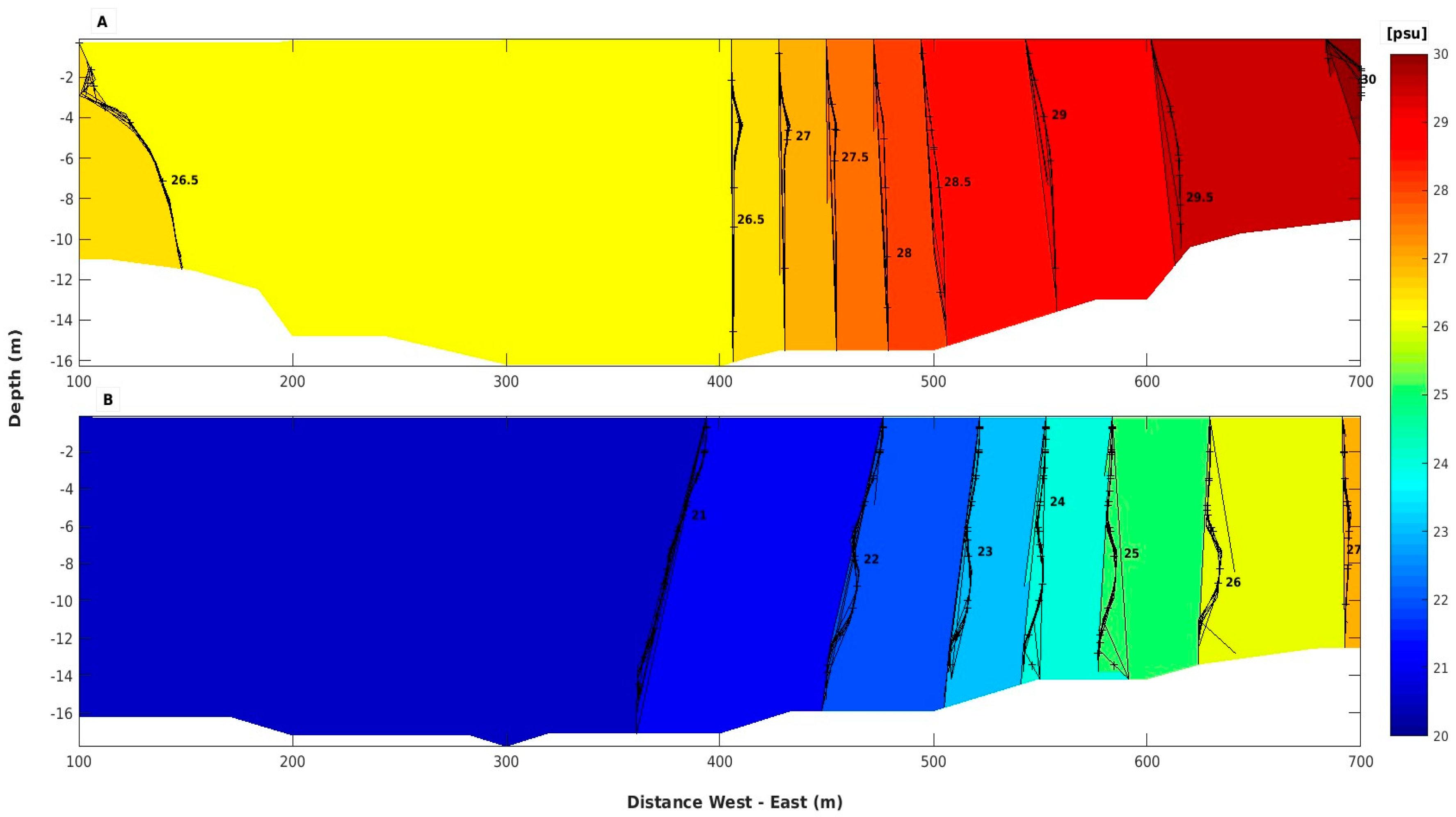
3.3. Changes in Salinity Stratification at the Mouth of the Estuary

Lateral stratification was evident between the jetties during the flood and ebb conditions, both at the surface and bottom for the old (Figure 15A,D,G,J) and new (Figure 15B,E,H,K) scenarios. Lateral stratification occurred at the estuary mouth, with higher salinity near the eastern than the western jetty. It was also evident that the range of salinity values between the jetties changed after the modification. In the old scenario, during flooding, the lateral salinity between the jetties ranged from 30–35 and was reduced to 23–27 after the jetty modification. During the ebb conditions, the lateral salinity values changed from 27–30 to 20–25 after the jetty modification.
After the changes in the jetty configuration, the lateral stratification time was reduced. During the flood flow at the same time step (Figure 15A,D), more salted water near the eastern than the western jetty was verified in the old configuration. In contrast, in the new configuration (Figure 15B,E), the flood current already dominated every navigation channel. On the other hand, in the western jetty during the ebb time step with the new configuration (Figure 15H,K), the estuary lost less saline water (approximately 20) to the ocean. In the old configuration (Figure 15G,J), the estuary lost a greater quantity of saline water (approximately 25).
The differences in salinity between the old and new scenarios for the flood results were significant in the region adjacent to the coast and in the shallow regions inside the estuary. A decrease of up to 15 units in the salinity was estimatedin the coastal and shallow embayments, and a decrease of approximately 5 was estimated in the navigation channel (Figure 15C,F). During the ebb flow, the highest differences were along the navigation channel and the coastal plume, with a decrease of approximately 7 units of salinity (Figure 15I,L). No changes were evident in the eastern coastal region.
Figure 16 presents the vertical cross sections of salinity between the jetties at point P1 (Figure 1), during the ebb time step of Figure 15G,H, for the old (Figure 16A) and the new configuration (Figure 16B). Salinity values presented a vertical mixed structure and horizontal stratified water column in both configurations. The horizontal structure from the western jetty to the eastern jetty showed salinity values ranging from 26.5 to approximately 30 in the old scenario (Figure 16A) and from approximately 20 to 27 in the new scenario (Figure 16B). The lateral salinity gradient was approximately 3.5 units in the old jetty configuration and approximately 7 in the new configuration. Results demonstrated a characteristic lateral salinity gradient with more salted water in the eastern side than in the west during the NE winds.
The ebb flow velocities were approximately twice the flood intensities between the jetties, but the center ebb velocity was highest with values above −6 m s−1 (Figure 17). The ebb current velocities were reduced in the western jetty and eastern jetty. In contrast, the flood velocity was more intense from the center of the channel to the eastern jetty, with currents faster than 2 m s−1. The ebb velocities were more intense from August to October. The velocity intensity for both the ebb and flood conditions was reduced by approximately 20% at the surface with jetty modification. At the bottom, the reduction was up to 50% at the center of the channel and near the eastern jetty.
Lateral stratification was also evident in the current velocity time series. The frequency distribution of the current velocities also revealed lateral stratification at the mouth of the estuary and indicated velocities higher than 6 m s−1 at the surface and close to 3 m s−1 at the bottom during flood conditions (Figure 18 and Figure 19). Reductions in the ebb and flood velocities occurred in the center of the channel and in the eastern channel from the old to new jetty configurations, both for the surface (Figure 18B,C,E,F) and the bottom (Figure 19B,C,E,F). In contrast, in the new western configuration, the intensification of the ebb and flow was registered at the surface (Figure 18A,D) and bottom (Figure 19A,D). The frequency of high velocities was reduced in the central area and the eastern side, while the maximum flood and ebb velocities were increased on the western side, both at the surface and bottom.
At the surface area by the eastern jetty (Figure 18C,F), the maximum ebb velocity decreased from approximately 5 to 4 m s−1, a reduction of approximately 20%. However, at the bottom (Figure 19C,F), the maximum flood and ebb velocities decreased from 2 to 1 m s−1, a reduction of 50%. Similar velocity behavior was verified at the bottom during the flood period in the center of the channel, but during the ebb period (Figure 19B,E), the maximum velocities did not exceed 2 m s−1 in the new configuration, in comparison with the 3 m s−1 registered in the old scenario, a reduction of approximately 33%. At the surface (Figure 18B,E), the maximum ebb velocity decreased from approximately 6 to 5 m s−1, a reduction of approximately 16%, and no visible change was verified in the flood velocities. In contrast, at the surface near the western jetty (Figure 18A,D), the maximum ebb velocities increased from approximately 3 m s−1 to more than 5 m s−1 from the old to the new scenario (an increase of 66%). In the flood stage, the velocities doubled in intensity, from approximately 1 to 2 m s−1 (an increase of 100%). At the bottom (Figure 19A,D), the velocities up to 1 m s−1 and higher than 1 ms−1 doubled in frequency of occurrence in the flood and ebb periods, respectively.
Changes in the jetty configuration also promoted changes in the angle of incidence of the current velocity from the old to the new configuration, which was more evident in the western jetty. The angle of incidence of the ebb flow from the western jetty changed from W to NW, while the angle of incidence of the flood flow changed from SE to E (Figure 18A,D, and Figure 19A,D).

4. Discussion

This paper applied the TELEMAC-3D model to investigate the effects of the recent modernization work on the jetties of the Patos Lagoon mouth on the hydrodynamics of the system during the high discharge period in 2002–2003 (El Niño) and the low discharge period in 2011–2012 (La Niña). As the model results agreed well with the in situ data during the calibration and validation processes, the model was considered adequate for predicting the current velocity, water level and salinity behavior, both at the bottom and surface, for both configurations (new and old).
The hydrodynamic characteristics of estuaries are subject to several forces that could determine their spatio-temporal variability [27,37]. In this study, we presented changes in the hydrodynamic behavior of the Patos Lagoon estuary due to alterations in the jetty configurations and the entrance channel to Patos Lagoon. The study evaluated changes in currents and salinity excursion and distribution in the scenarios with different geomorphologies, freshwater inflow and local and non-local wind effects. The scenarios of high and low river discharge were used since freshwater inflow is a major controlling force of the dynamics of the Patos Lagoon [21,24], and the region is subject to El Niño/La Niña cycles [20].
These periods of extreme high and low discharge were accompanied by dynamic winds that predominantly came from the N and S quadrants, which were also important for the local hydrodynamics [19,38], mainly when discharge was lower than 3000 m3 s−1 [21,24].
Contrary to what was anticipated and used as the motivation for the jetty elongation and the narrowing of its mouth, results revealed a decrease in the current velocity throughout the estuary and in the inner lagoon after the alteration. A more significant decrease of approximately 20% was estimated at the estuary mouth and has also been observed by [14]. These authors suggested that the causes could be related to changes in the dynamics of coastal currents and in the coastal plume direction and the intensification of the recirculation zones, which occur at the north and south of the jetties. Other factors, such as the prolongation and intensification of the funnel [11], and the convergence of the jetty edges, could have contributed to the decrease in the current velocity. In [24], the authors assumed that changes in the morphology induced by dredging, embankment, jetty or bridge construction can alter wave propagation, modify vertical salinity stratification, and decrease or increase the saltwater penetration into the estuary.
In estuaries that present a significant contribution of freshwater, salinity decreases with high river flow, reflecting the effect of river discharge on the salinity distribution in coastal environments [27,39]; the opposite effect is observed for low discharges. The model results showed decreasing salinity with the increase of discharge during 2002–2003, and the opposite was verified during 2011–2012. Similar results were observed during 1997–1998 and 2011, which were high discharge periods [18,19,20,27], where the salinity decrease was followed by high precipitation associated with the El Niño events and NE wind, which promoted intense ebb flows, making the estuarine region sometime unsalted. This event may persist for months because the continental waters are forced towards the mouth, preventing the salinization of the lagoon [24]. In contrast, salinization of Patos Lagoon occurred during 2011–2012, and [27] and [38] studied the 1988 and 2006 La Niña events, respectively, and attributed the enhanced saltwater intrusion to the combination of low precipitation and SW wind and reported that the oligohaline limit reached approximately 180 km, from the Patos Lagoon mouth, near point P7 (Figure 1), which was in agreement with our results.
The jetty modernization work changed the salinity distribution by reducing saltwater intrusion. The direct analyses of the daily salinity time series revealed strong variability in the salinity patterns on a timescale of approximately 16 days. This modulation was characteristic of the passage of meteorological fronts over the area [21,34]. Significant differences in the power variability from the estuary entrance region to the northern limit of the lagoon were registered. Near the estuary mouth for both high and low discharge simulations, the global power spectrum was approximately one order of magnitude higher than in the estuarine limit and close to the Guaíba River mouth in the old configuration. However, in the new configuration, the global power spectrum decreased two orders of magnitude for the same locations. This behavior can be associated with the reduction of the most energetic events in the exchange region between the estuary and the coastal regions [34] as a consequence of the jetty modification.
The power variation analyses also showed that the local wind close to the Patos Lagoon mouth was the main factor that controlled salinity propagation in the coastal and southern estuarine regions, with the direct transfer of momentum to the water column [34]. On the other hand, from the north of the lagoon towards the estuary, the discharge-controlled salinity events. Previous studies based on in situ measurements and model results have noted that the Patos Lagoon circulation was mainly controlled by the combination of discharges and local and non-local wind action [19,21,23,34].
The salinity signal lost strength and significantly decreased in power towards the lagoon as a consequence of the reduced saltwater intrusion with the new configuration compared to the old jetty configuration. The modification of the jetty configuration also seemed to contribute to the reduction of the propagation of the tides into the estuary.
The lateral flow stratification characterized by flooding near the eastern jetty and ebb near the western jetty in the Patos Lagoon access channel was already present in the old jetty configuration [23]. This behavior was attributed to the asymmetry of the jetty length and the anthropogenic dredging activity in the navigation channel located near the eastern jetty and the channel depth [23,24]. The jetty modification maintained this behavior but decreased the occurrence of lateral stratification by half. Despite the presence of lateral stratification, the vertical water column presented a mixed characteristic, which is typical of estuaries [21,40], suggesting that when the lateral density gradient was at a maximum, vertical mixing was supposed to be less efficient.
With the new jetty configuration, the higher velocities estimated from the center of the channel to the eastern jetty during the ebb and flood currents were reduced. Associated with the other findings of this study, this trend highlights the decrease in current velocity, which was mainly verified near the estuary mouth. The western shift in the ebb and flood propagation angle was also visible and indicated a result of the engineering work, as suggested by [9] at the eastern coast of Bandar Abbas. Changes in the propagation current velocity direction changed the bed level evolution and induced sedimentation on the eastern jetty and erosion on the western jetty.
The influence of the jetty configuration on the saltwater intrusion was reflected in the flow characteristic. The indentation of the maximum saltwater intrusion on the new configuration contributed to the reduced transfer of momentum and promoted stratification by weak vertical shear action at the new, less than the old, configuration [23]. The weak action of the hydrodynamic agents and the condition that was directly related to lower depth and smaller tidal range have as a consequence weaker turbulence and tidal current action [37].
The results supported the hypothesis that the jetty modernization work caused changes in the Patos Lagoon hydrodynamics. As a consequence, changes in the transport and distribution of the estuarine properties and organisms in the whole lagoon could also be expected. In [10], the authors explained that changes in the circulation pattern could also negatively impact the navigation of large vessels and the pollution and sedimentation processes (by the reduction of the ebb currents and natural dredging in the access channel). Other effects, such as the migration of the tidal delta as a result of changes in the morphodynamics of the central channel and the infilling or formation of banks on the jetty sides, which could influence the maintenance of adequate water depth, were mentioned by [2] after the Ribadeo port expansion in Spain. Ecologically, the reduction of saltwater intrusion and sporadic saltwater peak events could greatly impact the entrance of oceanic organisms, which contribute to the increase of recruitment of estuarine dependent species and are essential for maintaining the fish stocks in the Rio Grande do Sul coastal region.
The presence of lateral stratification in the access channel was expected to be an important factor because it influences the stratification, mixing, and distribution of the organisms and properties in areas of the estuary. In [40], the authors considered that this effect occurs when a maximum lateral density gradient is observed and that the transverse mixing should be less efficient. This lateral stratification could define the distribution of eggs, larvae, sediments and other water properties during the ebb and flood currents, indicating possible locations of maximum and minimum concentrations.

5. Conclusions

The effect of the recent modernization works on the jetties at the access channel to the Port of Rio Grande port was investigated applying the TELEMAC-3D numerical modeling in extreme freshwater discharge conditions. The validation and calibration demonstrated that the applied model provided acceptable results.
The jetty modernization did not contribute to the propagation of the inflow and outflow through the narrow inlet, and the ebb and flood current velocity ranges were reduced by approximately 20%. With the new configuration, the saltwater intrusion decreased, sporadic salinity peaks disappeared, and the strength of the salinity signal decreased by more than one order of magnitude in the interior of the estuary and lagoon.
Changes in the mouth configuration contributed to the partial centralization of the access channel flow, reducing the duration of lateral stratification by one-third.
The modifications induced a reduction of approximately 20% for the ebb and flood surface velocities, and a reduction of over 50% in the bottom velocities was estimated near the eastern jetty. A relative increase in the current velocity at the western jetty during flooding was estimated. The modernization of the jetties also changed the flow characteristic into the estuary by altering the angle of propagation of the ebb and flood currents near the western jetty.

Supplementary Materials

The following are available online at https://www.mdpi.com/2073-4441/12/11/3197/s1, Figure S1: Time series of river discharge and wind for the period between August 2011 and July 2012. South (North) winds are positive (negative) (L). Current velocity time series at surface (left) and bottom (right) at points P6 (M and N), P7 (O and P), P8 (Q and R) for old (black line) and new (red line) jetties configuration during August 2011 and July 2012. Positive (negative) values denote flood (outflow). The blue line in all plots shows the difference between the old and new jetties configuration, Figure S2: Time series (top) of river discharge and wind for the period between August 2011 and July 2012. South (North) winds are positive (negative) (L). Salinity time series at surface (left) and bottom (right) at points P6 (M and N), P7 (O and P), P8 (Q and R), of old (black) and new (red) jetties configuration during 2011–2012 (La Niña). The blue line in all plots shows the difference between the old and new jetties configuration, Table S1: Parameters used in the model set-up.

Author Contributions

M.H.P.A. conceived and designed the experiments, performed the experiments, analyzed the data, prepared figures and/or tables, authored and reviewed drafts of the paper, approved the final draft. E.H.F. and J.H.M. conceived and designed the experiments, authored and reviewed drafts of the paper, approved the final draft. All authors have read and agreed to the published version of the manuscript.

Funding

This research was partially funded by the Brazilian Long-Term Ecological Research Program (PELD) from CNPq (Proc.441492/2016-9) and the Fundação de Amparo à Pesquisa do Estado do Rio Grande do Sul (Proc. 16/2551-0000102-2).

Acknowledgments

The authors would like to acknowledge CAPES (Coordenação de Aperfeiçoamento Pessoal de Ensino Superior) for sponsoring the first author’s (M.H.P.A.) PhD’s grant through the Programa de Pós-Graduação Ciência para o Desenvolvimento (PGCD), and CNPq (Conselho Nacional de Desenvolvimento Científico and Tecnológico) for the research grants 307602/2014-1 (E.H.F.) and Proc. 310047/2016-1 (J.H.M.). We are also grateful to the LOCOSTE (Laboratório de Oceanografia Costeira e Estuarina) team for giving support during this research and to Osmar Moller for providing the in situ data used for the calibration and validation of TELEMAC-3D model.

Conflicts of Interest

The authors declare no conflict of interest.

References

  1. Adger, W.N.; Hughes, T.P.; Folke, C.; Carpenter, S.R.; Rockstrom, J. Social-Ecological Resilience to Coastal Disasters. Science 2005, 309, 1036–1039. [Google Scholar] [CrossRef] [Green Version]
  2. Prumm, M.; Iglesias, G. Impacts of port development on estuarine morphodynamics: Ribadeo (Spain). Ocean Coast. Manag. 2016, 130, 58–72. [Google Scholar] [CrossRef] [Green Version]
  3. Zhao, J.; Guo, L.; He, Q.; Wang, Z.B.; Maren, D.S.V.; Wang, X. An analysis on half centurry morphological changes in the Changjiang Estuary: Saptial variability under natural processes and human intervention. J. Mar. Syst. 2018, 181, 25–36. [Google Scholar] [CrossRef] [Green Version]
  4. Braverman, M.S.; Acha, E.M.; Gagliardini, D.A.; Rivarossa, M. Distrubution of Whitemouth croaker (Micropoginias furnieri, Desmarest 1823) larvae in the Rio de La Plata estuarine front. Estuar. Coast. Shelf Sci. 2009. [Google Scholar] [CrossRef]
  5. Salvador, N.L.A.; Muelbert, J.H. Environmental variability and body condition of Argentine menhaden larvae, Brevoortia pectinata (Jenyns, 1842), in estuarine and coastal waters. Estuaries Coasts 2019, 42, 1654–1661. [Google Scholar] [CrossRef]
  6. Abreu, P.C.; Odebrecht, C.; Niencheski, L.F. Nutrientes Dissolvidos. In O Estuário da Lagooa dos Patos: Um século de Transformações; Seeliger, U., Odebrecht, C., Eds.; FURG: Rio Rrande, Brazil, 2010; 180p, ISBN 978-85-7566-144-4. [Google Scholar]
  7. Able, K.W. A re-examination of fish estuarine dependence: Evidence for connectivity between estuarine and ocean habitats. Estuar. Coast. Shelf Sci. 2005, 64, 5–17. [Google Scholar] [CrossRef]
  8. Sheaves, M.; Baker, R.; Nagelkerken, I.; Connolly, R.M. True value of estuarine and coastal nurseries for fish: Incorporating complexity and dynamics. Estuaries Coasts 2015, 38, 401–414. [Google Scholar] [CrossRef] [Green Version]
  9. Ghashemizadeh, N.; Tajziehchi, M. Impact of Long Jetty on Shoreline Evaluation (Case Study: Eastern Coast of Bandar Abbas). J. Basic Appl. Sci. Res. 2013, 1256–1266. [Google Scholar]
  10. Azarmsa, S.A.; Esmaeili, M.; Khaniki, A.K. Impacts of Jetty construction on the wave heights of theKiashahr lagoon. Aquat. Ecosyst. Health Manag. 2009, 12, 358–363. [Google Scholar] [CrossRef]
  11. Yuk, J.H.; Aoki, S. Impact of Jetty construction on the current and Ecological Systems in the Estuary with a Narrow Inlet. J. Coast. Res. 2007, 784–788. [Google Scholar]
  12. Martelo, A.F.; Trombetta, T.B.; Lopes, B.V.; Marques, W.C.; Moller, O.O. Impacts of dredging on the hydromorphodynamics of the Patos Lagoon estuary, southern Brazil. Ocean Eng. 2019, 188. [Google Scholar] [CrossRef]
  13. Esteves, L.S.; Da Silva, A.R.P.; Arejano, T.B.; Pivel, M.A.G.; Vranjac, M.P. Coastal Development and Human Impacts Along the Rio Grande do Sul Beaches, Brazil. Journal of Coastal Research SI 35. In Proceedings of the Brazilian Symposium on Sandy Beaches, Morphodynamics, Ecology, Uses, Hazards and Management, Itajaí, Brazil, 3–6 September 2003; pp. 548–556. [Google Scholar]
  14. Silva, P.D.; Lisboa, P.V.; Fernandes, E.H. Changes on the fine sediment dynamics after the Port of Rio Grande expansion. Adv. Geosci. 2015, 39, 123–127. [Google Scholar] [CrossRef] [Green Version]
  15. Lisboa, P.V.; Fernandes, E.H. Anthropogenic influence on the sedimentary dynamics of a sand spit bar, Patos Lagoon Estuary, RS, Brazil. J. Integr. Coast. Zone Manag. 2015, 15, 35–46. [Google Scholar] [CrossRef]
  16. Kjerfve, B.; Magill, E.K.E. Comparative oceanography of coastal lagoons. In Estuarine Variability; Wolfe, D.A., Ed.; Academic Press: New York, NY, USA, 1986; pp. 63–81. [Google Scholar]
  17. Castelão, R.M.; Moller, O.O. A modeling study of Patos Lagoon (Brazil) Flow response to idealized wind and river discharge dynamical analysis. Braz. J. Oceanogr. 2006, 54, 1–17. [Google Scholar] [CrossRef]
  18. Moller, O.O.; Castello, J.P.; Vaz, A.C. The Effect of river discharge and winds on the interannual variability of the Pink Shrimp Farfantepeneaus paulensis Production in Patos Lagoon. Estuaries Coasts 2009, 787–796. [Google Scholar] [CrossRef]
  19. Fernandes, E.H.L.; Dyer, K.R.; Moller, O.O.; Niencheski, L.F.H. The Patos Lagoon hydrodynamics during El Niño event (1998). Cont. Shelf Res. 2002, 22, 1699–1713. [Google Scholar] [CrossRef]
  20. Garcia, A.M.; Vieira, J.P.; Winemiller, K.O. Effects of 1997-1998 El-Niño on the dynamics of the shallow-water fish assemblage of the Patos Lagoon Estuary (Brazil). Estuar. Coast. Shelf Sci. 2003, 57, 489–500. [Google Scholar] [CrossRef]
  21. Moller, O.O.; Castaing, P.; Salomon, S.; Lazure, P. The Influence of Local and Non-local Forcing Effects on the Subtidal Circulation of Patos Lagoon. Estuaries 2001, 24, 297–311. [Google Scholar] [CrossRef]
  22. Fernandes, E.H.L.; Tapia, I.M.; Dyear, K.R.; Moller, O.O. The attenuation of tidal and subtidal oscillations in the Patos Lagoon Estuary. Ocean Dyn. 2004, 54, 348–359. [Google Scholar] [CrossRef]
  23. Fernandes, E.H.L.; Dyer, K.R.; Moller, O.O. Spatial Gradients in Flow of Southern Patos Lagoon. J. Coast. Res. 2005, 21, 759–769. [Google Scholar] [CrossRef]
  24. Moller, O.O.; Fernandes, E.H.L. Hidrologia e Hidrodinâmica. In O Estuário da Lagoa dos Patos: Um século de Transformações; Seeliger, U., Odebrecht, C., Eds.; FURG: Rio Grande, Brazil, 2010; pp. 17–27. ISBN 978-85-7566-144-4. [Google Scholar]
  25. Marques, W.C.; Monteiro, I.O.; Fernandes, E.H. Numerical modeling of Patos Lagoon plume, Brazil. Cont. Shelf Res. 2009, 29, 556–571. [Google Scholar] [CrossRef]
  26. Marques, W.C.; Fernandes, E.H.L.; Rocha, L.A.O. Straining and advection contributions to the mixing process in the Patos Lagoon estuary, Brazil. J. Geophys. Res. 2011, 115, C03016. [Google Scholar] [CrossRef]
  27. Seiler, L.M.N.; Fernandes, E.H.L.; Martins, F.; Abreu, P.C. Evolution of hydrologic influence on water quality variation in a coastal lagoon through numerical modeling. Ecol. Model. 2015, 314, 44–61. [Google Scholar] [CrossRef]
  28. TELEMAC 3D Model Information. Available online: www.opentelemac.org (accessed on 16 September 2020).
  29. Hervouet, J.M. Hydrodynamics of Free Surface Flows: Modeling with the Finite Element Method; Wiley: Chichester, UK, 2007. [Google Scholar]
  30. Vaz, A.C.; Möller, O.O.; Almeida, T.L. Análise quantitativa da descarga dos rios afluentes da Lagoa dos Patos. Atlântica 2006, 28, 13–23. [Google Scholar]
  31. Discharge Data. National Water Agency. Available online: http://www.ana.gov.br (accessed on 16 September 2020).
  32. Salinity and Temperature Data. Hybrid Model Coordinate Oceanic. Available online: https://hycom.org/ (accessed on 16 September 2020).
  33. Wind Data. European Center for Medium-Range Weather Forecasts. Available online: http://www.ecmwf.int (accessed on 16 September 2020).
  34. Marques, W.C.; Fernandes, E.H.L.; Moller, O.O. Straining and advection contributions to the mixing process of the Patos Lagoon coastal plume, Brazil. J. Geophys. Res. 2010, 115, C06019. [Google Scholar] [CrossRef] [Green Version]
  35. Walstra, L.; Van Rijn, L.; Blogg, H.; Van Ormondt, M. Evaluation of a Hydrodynamic Area Model Based on the Coast3d Data at Teignmouth 1999; Report TR121-EC MAST Project No. MAS3-CT97-0086; HR: Wallinford, UK, 2001; pp. D4.1–D4.4. [Google Scholar]
  36. Torrence, C.; Compo, G.P. A Practical guide of wavelet analyses. Bull. Am. Meteorol. Soc. 1998, 79, 61–79. [Google Scholar] [CrossRef] [Green Version]
  37. Freitas, P.P.; Menezes, M.O.B.; Schettini, C.A.F. Hydrodynamics and Suspended Particulate matter transport in a shallow and highly urbanized estuary: The Cocó Estuary, Fortaleza, Brazil. Rev. Bras. De Geofísica 2015, 33, 579–590. [Google Scholar] [CrossRef] [Green Version]
  38. Odebrecht, C.; Abreu, P.C.; Moller, O.O., Jr.; Niencheski, I.F.; Proença, L.A.; Torgan, L.C. Drought Effect on Pelagic Properties in the shallow and turbid Patos Lagoon, Brazil. Estuaries 2005, 28, 675–685. [Google Scholar] [CrossRef]
  39. Azevedo, I.C.; Bordalo, A.A.; Duarte, P. Influence of freshwater inflow variability on the Douro estuary primary productivity: A modelling study. Ecol. Model. 2014, 272, 1–15. [Google Scholar] [CrossRef]
  40. Dyer, K.R. Estuarine flow interaction with topography—Lateral and longitudinal effects. In Estuarine Circulation; Neilson, B.J., Kuo, A., Brubaker, J., Eds.; Human Press: Tototowa, NJ, USA, 1989; pp. 39–59. [Google Scholar]
Figure 1. The study site located in Southeast South America, depicting (A) The Patos Lagoon and its main tributaries, where the three blue points (E1—São Lourenço, E2—Arambaré and E3—Ipanema) indicate the position where in situ water level data were obtained inside the lagoon, and the red point (N) indicates where current velocity was obtained from the coastal region. The dotted line indicates the estuarine limit (Ponta da Feitoria). (B) Patos Lagoon estuary, where eight back points (P1–P8) show the location where the model results were extracted and P2 indicates the Praticagem position where salinity and current velocity data were obtained in the estuarine area.
Water 12 03197 g001
Figure 2. Southern Oscillation Index (SOI) and discharge anomalies for the 2002–2012 period (top and middle panels). Black rectangles represent periods of Patos Lagoon high discharge during El-Niño (bottom left) and low discharge during La-Niña (bottom right), the years that were simulated in this study.
Water 12 03197 g002
Figure 3. (A) The model domain and the finite elements grid with the initial and boundary conditions applied to the old and new configuration. The lower Patos Lagoon estuary in the (B) old and (C) new jetty configuration.
Water 12 03197 g003
Figure 4. Calibration exercise—comparison between modeled (red line) and measured (black line) current velocity at the surface (left panel) and bottom (right panel), in the old (A,B) and new (C,D) jetty configurations.
Water 12 03197 g004
Figure 5. Validation exercise comparison between modeled (red line) and measured (black line) current velocity, salinity and water elevation for the old jetty configuration. Surface velocity (A) and salinity (C) and bottom velocity (B) and salinity (D). (EG) water elevation for points E1 (São Lourenço), E2 (Arambaré) and E3 (Ipanema).
Water 12 03197 g005
Figure 6. Validation exercise comparison between modeled (red line) and measured (black line) salinity and water elevation for new jetty configuration. Surface (A) and bottom (B) salinity data. (CE) water elevation for points E1 (São Lourenço), E2 (Arambaré) and E3 (Ipanema), respectively.
Water 12 03197 g006
Figure 7. Time series of river discharge and wind for the period between April 2002 and March 2003. South (North) winds are positive (negative) (A). Calculated current velocity difference between results for the old and new jetty configuration at surface (left) and bottom (right) at points P1 (B,C), P2 (D,E), P3 (F,G), P4 (H,I) and P5 (J,K), between April 2002 and March 2003. Positive (negative) values denote inflow (outflow).
Water 12 03197 g007
Figure 8. Time series of river discharge and wind for the period between August 2011 and July 2012. South (North) winds are positive (negative) (A). Calculated current velocity difference between results for the old and new jetty configuration at surface (left) and bottom (right) at points P1 (B,C), P2 (D,E), P3 (F,G), P4 (H,I) and P5 (J,K) between August 2011 and July 2012. Positive (negative) values denote inflow (outflow).
Water 12 03197 g008
Figure 9. Time series of river discharge and wind for the period between April 2002 and March 2003. South (North) winds are positive (negative) (A). Calculated salinity difference between results for the old and new jetty configuration at surface (left) and bottom (right) at points P1 (B,C), P2 (D,E), P3 (F,G), P4 (H,I) and P5 (J,K), in 2002–2003 (El Niño).
Water 12 03197 g009
Figure 10. Spatial distribution of salinity during maximum flood (top panels) and maximum ebb (bottom panels) during the period of high discharge (2002–2003), considering the old (left) and new (center) scenarios and the calculated difference in salinity distribution (right). Results are presented for the surface (AC,GI) and for the bottom (DF,JL).
Water 12 03197 g010
Figure 11. (A,D,G,J) Time series of salinity and (B,E,H,K) wavelet power spectrum of the time series for the estuary entrance (P1, top 2 panels) and near estuary limit (P4, bottom 2 panels), during the high discharge 2002–2003 period for the old (A,B,G,H) and for the new (D,E,J,K) jetty configurations. Thick contour line enclosed regions of greater than 95% confidence. Dash-dot regions indicate the cone of influence. Dash-dot regions indicate the cone of influence where the edge effect become important (C,F,I,L). The global wavelet power spectrum of the time series and the dotted red line indicate the 95% confidence level.
Water 12 03197 g011
Figure 12. Time series (top) of river discharge and wind for the period between August 2011 and July 2012. South winds are positive, north winds are negative (A). Calculated salinity time series at surface (left) and bottom (right) at points P1 (B,C), P2 (D,E), P3 (F,G), P4 (H,I) and P5 (J,K), of old (black) and new (red) jetties configuration during 2011–2012 (La Niña). The blue line in all plots shows the difference between results for the old and new jetty configurations.
Water 12 03197 g012
Figure 13. Spatial distribution of salinity during maximum flood (top panels) and maximum ebb (bottom panels) during the period of low discharge (2011–2012), considering the old (left) and new (center) scenarios, and the calculated difference in salinity distribution (right). Results are presented for the surface (AC,GI) and for the bottom (DF,JL).
Water 12 03197 g013
Figure 14. (A,D,G,J) Time series of salinity and (B,E,H,K) wavelet power spectrum of the time series for the estuary entrance (P1, top 2 panels) and estuary limit (P5, bottom 2 panels), during the low discharge 2011–2012 period for the old (A,B,G,H) and for the new (D,E,J,K) jetty configurations. Thick contour line enclosed regions of greater than 95% confidence. Dash-dot regions indicate the cone of influence where the edge effect become important (C,F,I,L). The global wavelet power spectrum of the time series and the dotted red line indicate the 95% confidence level.
Water 12 03197 g014
Figure 15. Spatial distribution of salinity at the mouth of the estuary depicting changes in intensity and lateral stratification between the jetties during the high discharge period of 2002–2003. Flood (top panels) and ebb (bottom panels), for the old (left) and new (center) scenarios, and the calculated difference in salinity distribution (right) at the surface (AC,GI) and bottom (DF,JL).
Water 12 03197 g015
Figure 16. Vertical cross-section distribution of salinity during ebb flow at the estuary entrance (P1) from west (left) to east (right) jetties, for the old (A) and new (B) jetty configurations, during the high discharge period 2002–2003 (El Niño).
Water 12 03197 g016
Figure 17. Current velocity time series from three points between the jetties (point P1) for the old (black line) and the new (colored lines) jetty configurations, during the high discharge period of 2002–2003 (El Niño). The points are located at: first near the west jetty (top panel), second at the center of the channel (center panel) and third near the east jetty (bottom panel), both for surface (left panel) and bottom (right panel). Positive (negative) values denote inflow (outflow).
Water 12 03197 g017
Figure 18. Frequency distribution of current velocity and incidence angle at the surface for points at the west (A,D), center (B,E) and east (C,F) jetties in the estuary entrance (P1), for the old (top) and new (bottom) jetty configurations, during the high discharge period 2002–2003 (El Niño). Northward (southward) velocities denote outflow (inflow).
Water 12 03197 g018
Figure 19. Frequency distribution of current velocity and incidence angle at the bottom for points at the west (A,D), center (B,E) and east (C,F) jetties in the estuary entrance (P1), for the old (top) and new (bottom) jetty configurations, during the high discharge period 2002–2003 (El Niño). Northward (southward) velocities denote outflow (inflow).
Water 12 03197 g019
Table 1. Relative Mean Absolute Error (RMAE) results for hydrodynamic model validation.
ParametersPositionOld ConfigurationNew Configuration
RMAERMAE
VelocitySurface0.17-
Bottom0.18-
SalinitySurface0.060.09
Bottom0.300.05
ElevationE10.020.014
E20.080.03
E10.270.16
Publisher’s Note: MDPI stays neutral with regard to jurisdictional claims in published maps and institutional affiliations.

