Grapevine Sap Flow in Response to Physio-Environmental Factors under Solar Greenhouse Conditions

Abstract

Understanding transpiration responses to physiological and environmental factors is essential for efficient water management practices in greenhouse grapevine farms. To determine the driving factors of grapevine sap flow under solar greenhouse conditions in a typical cold climate, the sap flow, greenhouse micro-environmental conditions, and canopy details were measured and analyzed for the 2017–2018 growing season in Northeast China. The results showed that leaf area index controlled the upper boundary of sap flow rate (SFR). Correlations between SFR and meteorological factors obviously varied with time scales. Besides, the correlations at the hourly scale varied across the seasons. Photo-synthetically active radiation (PAR) was the primary control factor of sap flow, irrespective of time scale or season. The start and stop times of sap flow did not change with weather conditions, but SFR had broader peaks with higher peak values during sunny days. The diurnal variation of SFR lagged behind that of PAR, but remained ahead of those of VPD and temperature. Weather condition changed the sizes of the hysteresis loops, but not the rotation direction. The hydrological and physiological processes involved in sap flow are useful for refining transpiration models and improving water use efficiency in the greenhouse environment.

1. Introduction

Transpiration is a vital part of water transport in the soil–plant–atmosphere continuum and transpiration-related studies are crucial for understanding the physiological, hydrological, and ecological processes of plants [1]. Environmental coupling mechanisms of transpiration are important for improving the efficiency and sustainability of water resource management, both under irrigated and rain-fed conditions [2]. Among the various technologies for measuring transpiration in trees, heat-based sap flow methods have been widely used [3,4]. Based on previous studies, both physiological (e.g., leaf area, crown size, stem water potential, and stem shrinkage) and environmental factors (e.g., air temperature, precipitation, radiation, vapor pressure deficit, soil type, soil moisture and temperature, and groundwater level) influence sap flow to various extents. As a result, sap flow is often estimated using a variety of models with different forms and complexities considering both environmental and physiological factors [5,6].

Although countless studies on the investigation of physiological and environmental interactions involved in water movement process within tree trunks have been reported, the dominant factors influencing sap flow and their mode of sap flow-regulation are evidently different depending on tree species, climate conditions, management strategies, growth statuses, soil characteristics, etc. [7]. For example, the sap flow of Cryptomeria japonica was mainly controlled by VPD when wind speed was above 0.7 m s⁻¹, but the main driving factor changed to PAR when the wind speed was below 0.7 m s⁻¹ [8]. However, Tie et al. [9] indicated that PAR was always the key environmental factor controlling sap flow during the whole growth stage of Aspen (Populus davidiana) in a sub-humid mountainous catchment. Additionally, the influence of radiation on water usage by plants was reported to be strong during the wet season but much weaker in the dry season for plants in Brazilian semiarid coniferous forests [2] and Eucalyptus macrorhyncha in semiarid sites of south-eastern Australia [10].

Apart from massive studies on sap flow analyses conducted under natural planting conditions, numerous studies were also carried out in greenhouses, where the energy transmission pathway is changed artificially, leading to a pronounced micro-environment that is different from the outside. Regarding the sap flow feature and the underlying driving mechanism under greenhouse conditions, most studies focused on vegetables and flowers, such as tomato [11], cucumber [12], zucchini [13], impatiens ornamental plants [14], studies on trees showed that the controlling pattern of the influence factors on sap flow vary among tree species, climate, greenhouse type, and other factors. For example, Van Herk et al. [15] demonstrated that the sap flux of black spruce (Picea mariana (Mill.) BSP) planted in greenhouse was mainly driven by VPD and PAR. However, according to another study conducted in the Iberian Peninsula, the water usage of cherry trees grown in a greenhouse was mainly influenced by leaf stomatal conductance, which was directly linked to short radiation [16]. Similar observations were also noted in greenhouse apricot trees from south eastern Spain [17].

As the world’s largest greenhouse horticulture country, China has a greenhouse cultivation area of over 2.1 × 10⁶ hm², occupying 42.8% of the world’s total greenhouse cultivation area, mainly used to grow vegetables and fruits [18]. Because of the cold winter and large seasonal temperature difference, the effective accumulated temperature in years ranged from 1765 to 4395 °C in the Northeast China (Figure 1). Thus, the region is the core distribution zone of greenhouse horticulture in China. Pertaining to greenhouse horticulture, greenhouse grapevine accounts for a considerable portion. A comprehensive understanding of the interaction between grapevine sap flow and its influencing factors is vital for the sustainable development of the grape greenhouse industry in such high latitude region with cold weather and large temperature differences. Since previous relevant studies were mainly conducted in other regions [15,16,17], and studies from the local region were mainly targeted at other greenhouse plants [11,12]; necessary information for grapevine is lacking in Northeast China.

Therefore, this study focuses on enhancing the understanding of the special water use processes and water management systems in vineyards under solar greenhouse conditions in Northeast China. A systematic monitoring of grapevine physiology, micro-meteorological factors and the soil moisture conditions in greenhouse facilities during grapevine growth seasons were conducted for two consecutive years. The main objectives of the study include: (1) To analyze the main driving factors of sap flow at different time scales in greenhouse condition. (2) To investigate diurnal variation in sap flow and how its hysteresis is related to environmental factors under different weather conditions.

2. Materials and Methods

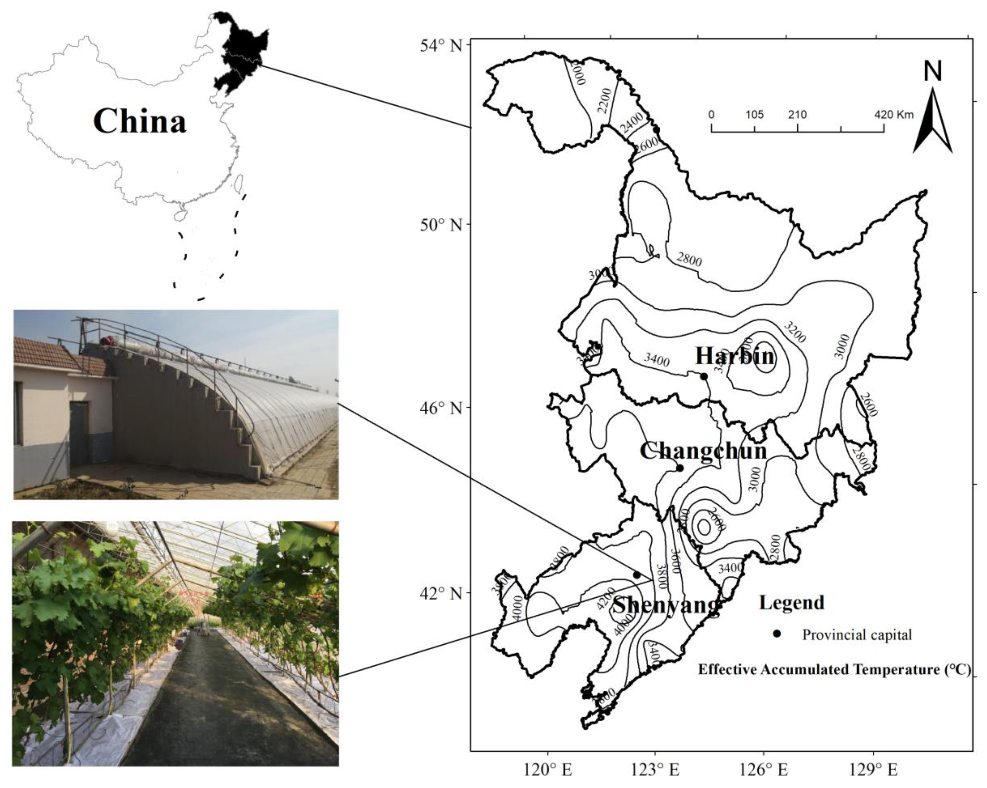
2.1. Study Site

The experiment was conducted in a solar greenhouse belonging to Shenyang Agricultural University in Northeast China (41°82′ N, 123°57′ E, Figure 1). The greenhouse type is a Liaoshen III style solar energy-saving greenhouse, a typical solar greenhouse type in Northeast China. Measurements were done during the whole growth stages in 2017 and 2018. The greenhouse was a single-sided parabolic lighting canopy with height of 3.5 m, length of 60 m and width of 9 m. An anti-aging PVC plastic film with non-dripping function was used to cover the top of the greenhouse and a rain-proof cotton quilt was used as insulator. The soil is sandy loam, with field moisture holding capacity of 22.3% and bulk density of 1.44 g cm⁻³. In total, 200 grapevines (Vitis vinifera L.cv.Muscat Ham-burg) were planted in two rows on 25 March 2016 at tree spacing of 0.5 m and row spacing of 4.5 m.

Before entering a new round of growing season every year, the grapevines were pruned to maintain trunk length within 4.0 ± 0.2 m and keep the number of fruit-bearing branches to 13–15 per tree at the end of March. The grapevine trunks were trained on trellis support of hockey stick shape (shown in Figure S1 as Supplementary Material). Water was supplied regularly by drip irrigation. More precisely, irrigation was done to 90% field moisture holding capacity whenever the soil water content in the root zone dropped below 70% field moisture-holding capacity. Urea fertilizer was applied at the early growth stage, before June, at 288 kg hm⁻². This was replaced with 600 kg hm⁻² of Germany compo special fertilizer (N = 14%, P = 3.5%, K = 24.9%) in subsequent applications, in June and July, corresponding to the fruit setting, enlargement, and coloring stages. The application amount of Germany compo special fertilizer was reduced to 450 kg hm⁻² from the fruit-ripening stage in August. All the cultivation practices, including but not limited to irrigation, fertilizer application, and disease and pest control, were the same for each plant and were based on local management standards.

2.2. Data Collection

2.2.1. Sap Flow

A total of 10 heathy and vigorous grapevines (see

Table 1. Characteristics of grapevines selected for sap flow measurement.

Grapevine Number	Trunk Length (m)		Average Length of Lateral Branch (m)		Number of Fruit Bearing Branches		Trunk Diameter (cm)
	2017	2018	2017	2018	2017	2018	2017	2018
1	3.81	3.83	0.65	0.61	14	13	1.09	1.15
2	3.82	3.89	0.59	0.65	14	15	1.03	1.09
3	3.85	3.88	0.61	0.70	15	15	1.09	1.18
4	3.84	3.81	0.64	0.60	15	14	1.04	1.08
5	4.01	4.17	0.59	0.53	15	15	1.07	1.12
6	3.84	3.82	0.61	0.62	15	14	1.09	1.17
7	3.87	3.88	0.66	0.6	15	13	1.01	1.06
8	3.82	3.83	0.62	0.64	14	14	1.06	1.12
9	3.89	3.93	0.58	0.62	14	15	1.05	1.13
10	3.89	3.81	0.61	0.59	15	15	1.04	1.09

Note that trunk diameter was measured at 30 cm aboveground.

for more details) with relatively straight trunks were randomly chosen as samples for sap flow measurement. Sap flow dynamics across the growth stages in 2017 and 2018 were monitored using the heat balance method. All the heat balance stem-flow gauge sensors (Flower 32-1K, SGB-9) (Dynamax, Inc., Houston, TX, USA) were installed on the main trunk of the grapevine at about 20 cm aboveground. Tin foil was used to wrap the sensors in order to prevent thermal exchange with the outside. Data were collected with CR1000 equipment (Campbell Scientific, Inc., Logan, UT, USA) at a time step of 10 min. Sap flow was calculated as described by Shackel et al. [19]

$$F=\frac{P\mathrm{in}-Qr-Qv}{\mathrm{Cp}\times \mathrm{dT}}$$

(1)

where F is the instantaneous sap flow rate (SFR; g h⁻¹); Pin is heat input (W); Qr is radial heat dissipation (W); Qv is vertical thermal conductivity (W); Cp is specific heat of water (4.186 J/g × C); and dT is average voltage of the two vertical thermocouples (°C).

The daily transpiration of the grapevine (T_c) was obtained by integrating sap flow throughout the day as follows

$$T_i={\displaystyle {\int }_0^{24}\mathrm{Fdt}}$$

(2)

$$T_c=\frac{\mathrm{m}\times {\displaystyle \sum _{i=1}^n{T}_i}}{1000\times n\times A}$$

(3)

where T_i is daily transpiration of a single grapevine (mm); T_c is the average daily transpiration of grapevines in the whole greenhouse (mm); A is the ground area of the vineyard (m²); n is the number of grapevines, for which, sap flow was measured (n = 10); i is the ith measured grapevine. m is the total number of grapevines in the vineyard.

2.2.2. Leaf Area Index (LAI)

During the whole study period, 30 shoots were randomly chosen from plants, for which, sap flow was monitored, to measure the shoot length, and the length and maximum width of all the leaves on the shoots. Besides, a total of 20 leaves on chosen shoots were randomly surveyed in the greenhouse for individual leaf area measurement. Specifically, leaf length and maximum width were measured. Subsequently, leaf photos were taken and leaf area was calculated with the software named “ImageJ”. The relationship between the leaf area of an individual leaf and the product of leaf length and maximum leaf width was derived from the data of 20 leaves. This relationship was then used to estimate the individual leaf area of all leaves on each marked shoot using the leaf length and maximum width data. This was next summed up to obtain the total leaf area for each shoot.

The correlation between the total leaf area of each shoot and shoot length was established using regression analysis (y = 0.0391x² + 9.371x + 82.492; R² = 0.84, p < 0.01). The length of every shoot on the 10 grapevines used for sap flow measurement was recorded and the corresponding total leaf area of all the shoots were calculated using the above correlation, and the shoot leaf area data summed up to get the total leaf area of the tree. For the experimental period, the above calculation was done once every 7–10 days and used to build the tree leaf area dynamics. At the same time, crown dimensions of the 10 plants were concurrently measured in four different directions, then, the canopy projection area was calculated as the area summation of different sub-sections of the canopy projection. The leaf area index (LAI) dynamics of each grapevine was obtained by dividing the leaf area by canopy projection area.

2.2.3. Soil Water Content

The SWC was measured using TDT (Time Domain Transmissometry) soil moisture sensors (Campbell Scientific, Inc., Logan, UT, USA). From personal investigation, root systems of the grapevines were mainly distributed in the 0–60 cm soil profile. Consequently, the SWC at 15, 30, and 50 cm depths were monitored at 10 randomly chosen sites in the greenhouse. The data were collected using the CR1000 (Campbell Scientific, Inc., Logan, UT, USA) at a time interval of 10 min, in the whole growth period.

2.2.4. Meteorology

Meteorological factors were continuously measured using the GRWS100 automatic weather stations (Campbell Scientific, Inc., Logan, UT, USA) in the greenhouse. Four climate factors were monitored—solar radiation (R_s, W m⁻²), photosynthetically active radiation (PAR, μmol m⁻² s⁻¹), air temperature (T, °C) and relative humidity (RH, %). R_s was monitored by CMP3 (Li-Cor, Lincoln, Nebraska, USA), PAR was measured by an LI-190R quantum sensor (Li-Cor, Lincoln, NE, USA), T and RH were measured by an HC2S3-L temperature and relative humidity probe (Rotronic AG, Grindelstrasse, Bassersdorf, Switzerland) with a radiation shield. All sensors were installed at 2 m above the ground. Additionally, three sensors were installed to measure outdoor temperature, humidity, and photosynthetically active radiation. Data were collected every 10 min using the CR1000. Vapor pressure deficit (VPD) was calculated from air temperature (T) and relative humidity (RH), as follows [20]

$$\mathrm{VPD}=0.611\times (1-\mathrm{RH})e^{\frac{1.27\times \mathrm{T}}{\mathrm{T}+278.8}}$$

(4)

Transpiration variable (VT), which is an integrated index, was introduced in the study. Since VPD accounts for over two-thirds, solar radiation accounts for most of the remaining one-third of total transpiration, VT was defined as a function of VPD and Rs, and was calculated as follows [9,21,22]

$$\mathrm{VT}=\mathrm{VPD}\times {(\mathrm{Rs})}^{1/2}$$

(5)

2.3. Data Analysis

Both linear and non-linear regression analysis were used to analyze the quantitative relationships between sap flow and physio-environmental factors. Regression analyses and data plotting were performed using SPSS ver. 19.0 and Origin ver. 9.1, respectively.

3. Results

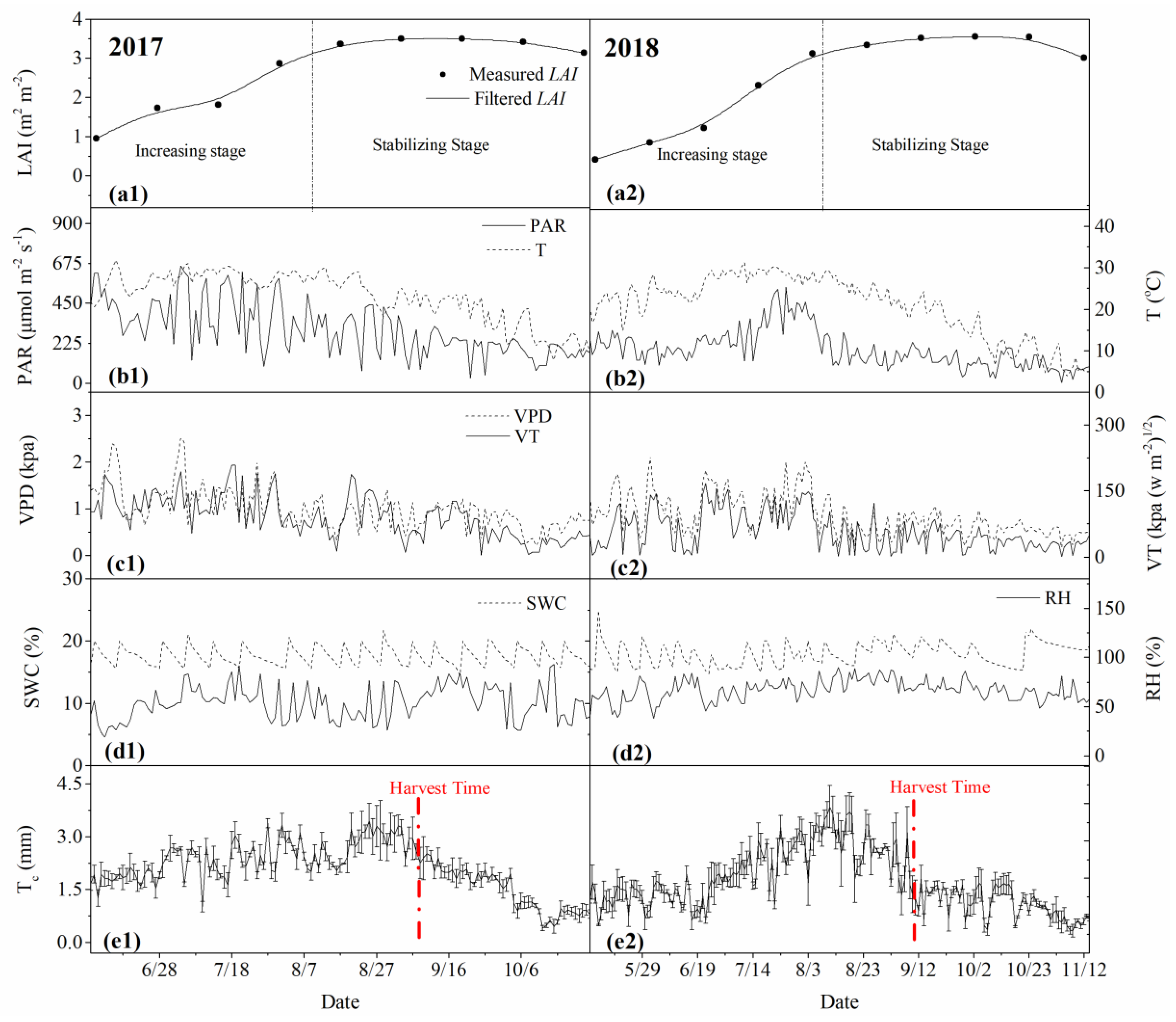
3.1. Dynamics of Physiological and Environmental Factors

Continuous diurnal variations of environmental factors (PAR, T, VPD, VT, SWC, and RH) in the greenhouse and the physiological indexes (LAI and transpiration) of grapevine during the 2017–2018 experimental period are shown in Figure 2.

LAI growth dynamics was roughly divided into two stages (Figure 2(a1,a2))—rapid increasing stage (including the flowering and fruit enlargement stages in April to July) and relative stabilizing stage (mainly refers to the fruit ripening and after harvesting stages in August to October). During the experimental period, T, PAR, VT, and VPD in the greenhouse were overall high before September, with peak values in July to August. Specifically, PAR fluctuated within 31.26–659.4 and 4.06–541 μmol m⁻² s⁻¹, respectively, in 2017 and 2018, with corresponding averages of 306.7 and 245.6 μmol m⁻² s⁻¹. Daily T averages in the greenhouse were 23.14 and 20.73 °C, respectively, in 2017 and 2018. Comparatively, greenhouse RH remained relatively stable during the whole experimental period, with averages of 53.30% and 66.76% in 2017 and 2018, respectively. This trend further led to relative narrow ranges of VPD, which changed within 0.21–2.5 kpa in 2017 and 0.17–2.12 kpa in 2018.

The transpiration of grapevine had obvious seasonal variation, with a unimodal peak (low-high-low) during the growing period from May to November (Figure 2(e1,e2)). During the early growth stage of grapevine in May, the daily transpiration was low, averaging 1.73 and 1.29 mm d⁻¹, in 2017 and 2018, respectively. With the expansion of leaves and the increase in LAI, daily transpiration gradually increased before peaking at the fruit ripening stage in August. During this period, the average transpiration reached 3.44 and 3.85 mm d⁻¹, respectively, in 2017 and 2018. This was followed by a drastic drop in the transpiration due to fruit harvest, for which period, the average transpiration dropped to 1.58 and 1.19 mm d⁻¹ respectively, in 2017 and 2018. The harvest time of 2018 was nine days later than that of 2017. After fruits harvesting, the grapevine leaves began to drop successively. In this process, the remaining leaves still consumed some water but they were much weaker.

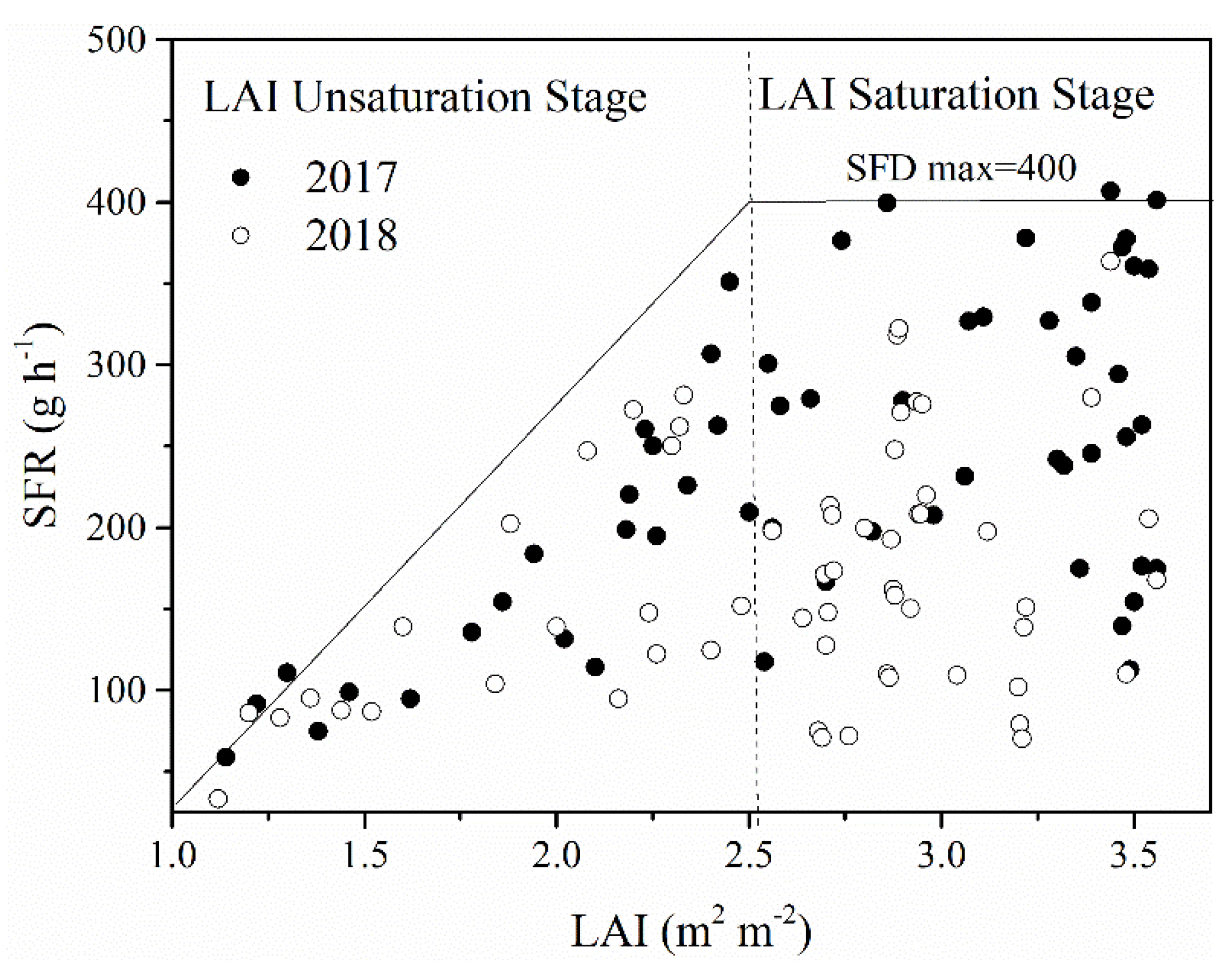
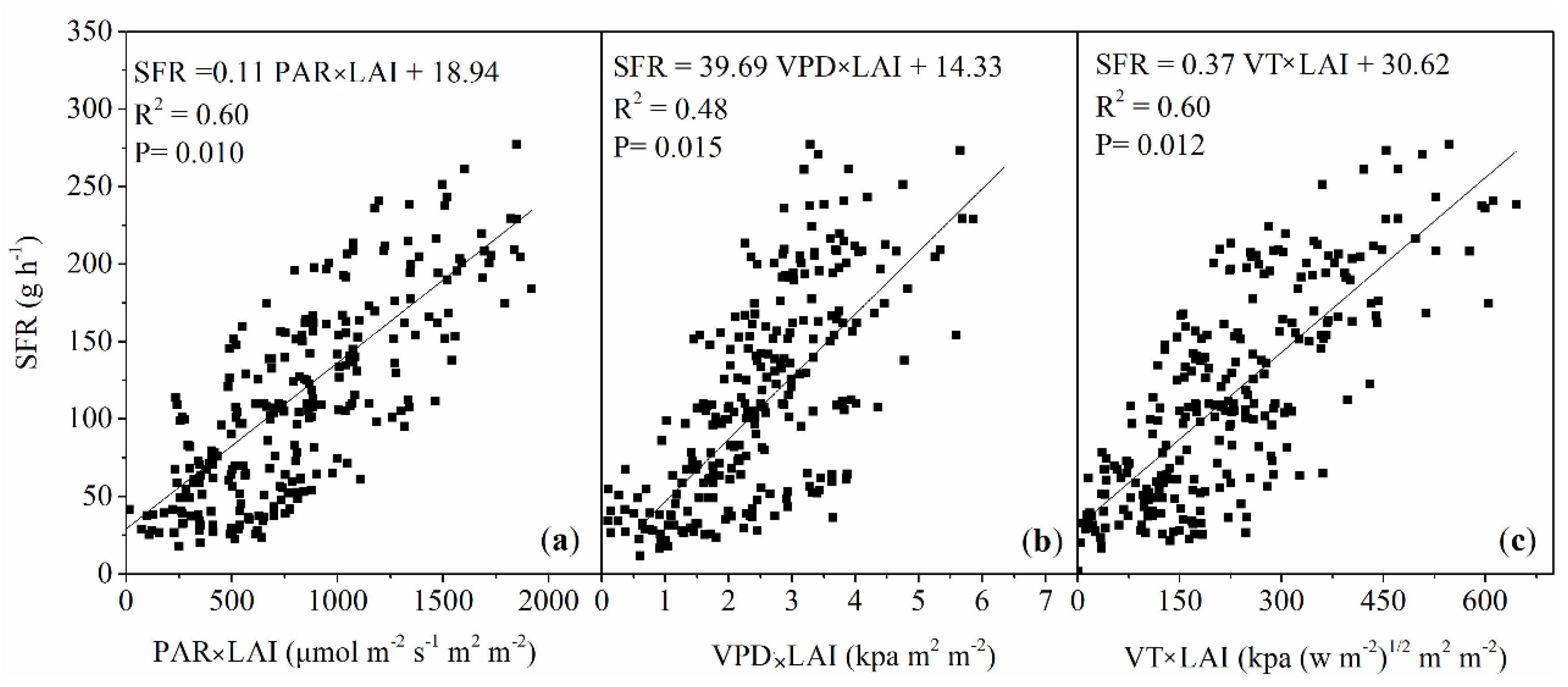
3.2. Control of Leaf Area Index on Sap Flow Rate

As in Figure 3, there were distinct responses of SFR to LAI for different phases. At the LAI unsaturated stage, the leaves grew vigorously; the SFR, overall, increased with increasing LAI for LAI < 2.5 m² m⁻², indicating that SFR was controlled by both LAI and other factors. At the LAI near saturation stage (corresponding roughly to fruit enlargement and coloring period), LAI finally stabilized at around 3.6 m² m⁻². There was no direct significant correlation between SFR and LAI for LAI > 2.5 m² m⁻². Under this condition, SFR largely fluctuated but had a stable maximum value of 400–450 g h⁻¹. Moreover, LAI determined the outlying envelope line of grapevine sap flow no matter at LAI saturation or unsaturated stages. There were some values distributed under the envelope line, because the transpiration of plants was not only controlled by LAI, it was also affected by the soil water and other meteorological factors [10,15].

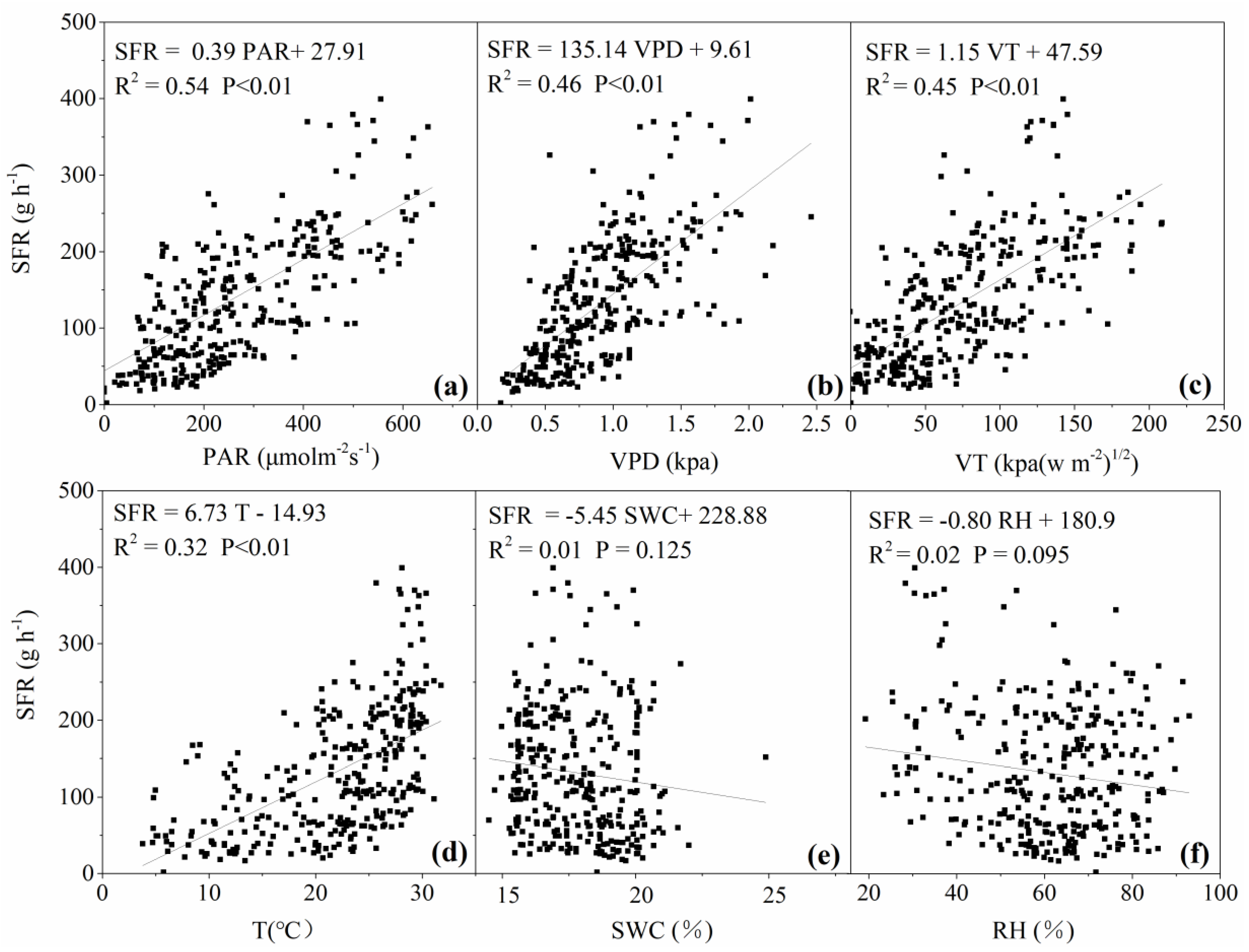
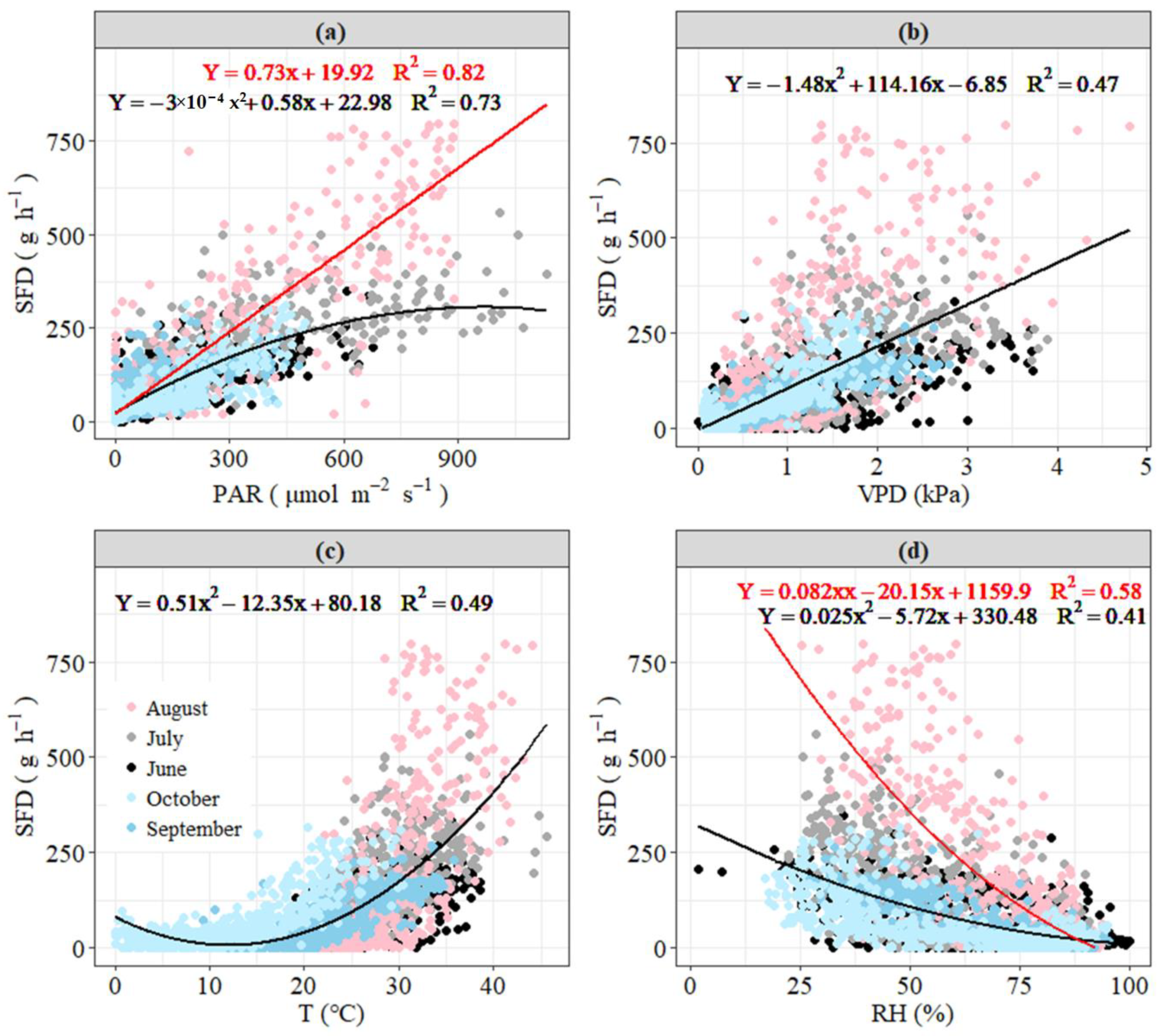
3.3. Response of Daily Sap Flow to Main Environmental Factors

To determine the response of sap flow in grapevine to environmental factors under greenhouse conditions, the correlations between the daily SFR and six major environmental factors (PAR, VPD, T, VT, SWC, and RH) were analyzed for the 2017 and 2018 growing periods (Figure 4). The results showed that the daily SFR was significantly positively correlated with PAR, T, VPD, and VT (p < 0.01), but had no significant correlation with SWC (p = 0.125) and RH (p = 0.095). The significance of the correlations between SFR and each of the meteorological factors was in the following order: PAR > VPD > VT > T > RH > SWC. Accordingly, PAR, VPD and VT were the most important environmental factors controlling sap flow in the grapevine at the daily time scale.

There is often a combination of environmental and physiological factors as integrated indicators in sap flow estimation, as such indicators are apparently more compatible with sap flow [9]. Based on the results from this study, the three most critical factors of SFR (PAR, VPD, and VT) were combined with the physiological factors of LAI to build three other integrated indicators (PAR × LAI, VPD × LAI, and VT × LAI) for further analysis (Figure 5). Regression relations with greater determination coefficient were noted between SFR and the integrated factors, compared with single environmental factors (0.48–0.60, as against 0.46–0.54). Among the three integrated factors, PAR × LAI had the highest estimation accuracy, with a determination coefficient of 0.60.

3.4. Response of Hourly Sap Flow to Climatic Factors and Seasonal Variability

To analyze the relationship between SFR and the main influencing factors, regression analysis was done for SFR and PAR, VPD, T, and RH, at an hourly scale, considering the variabilities across the seasons (Figure 6). SFR had good positive correlations with the PAR for each month. The plots in other months, except August, followed an overall consistent trend (parabolic function), which had an increasing phase with increasing PAR and a stable phase for PAR greater than 600 μmol m⁻² s⁻¹ (R² = 0.73). On the contrary, the plots for August had a clear linear correlation (R² = 0.82) with no insensitive change in SFR. It implies that even if PAR exceeds 600 μmol m⁻² s⁻¹, the stomata can remain largely open in August. This is beneficial for carbon assimilation and favor fruit-ripening quality. This holds true for the different diurnal changes in stomatal conductance, photosynthetic rate, and transpiration rate across different seasons, as shown in Figure S2, which suggested that the overall diurnal course of the three indexes was higher in August than in any other month. Similar to PAR, the correlation between hourly SFR and RH varied with season. Both plots for August and the other months followed a parabolic curve, but the plots for August (R² = 0.58) decreased more rapidly with increasing RH than for the other months (R² = 0.41). This also agreed well with the diurnal stomatal conductance, for which the decreasing trend after noon was sharper in August than in other months (Figure S2). Comparatively, plots of SFR against VPD or T for all the months had roughly the same parabolic curve (R² = 0.47 and 0.49 for VPD and T, respectively).

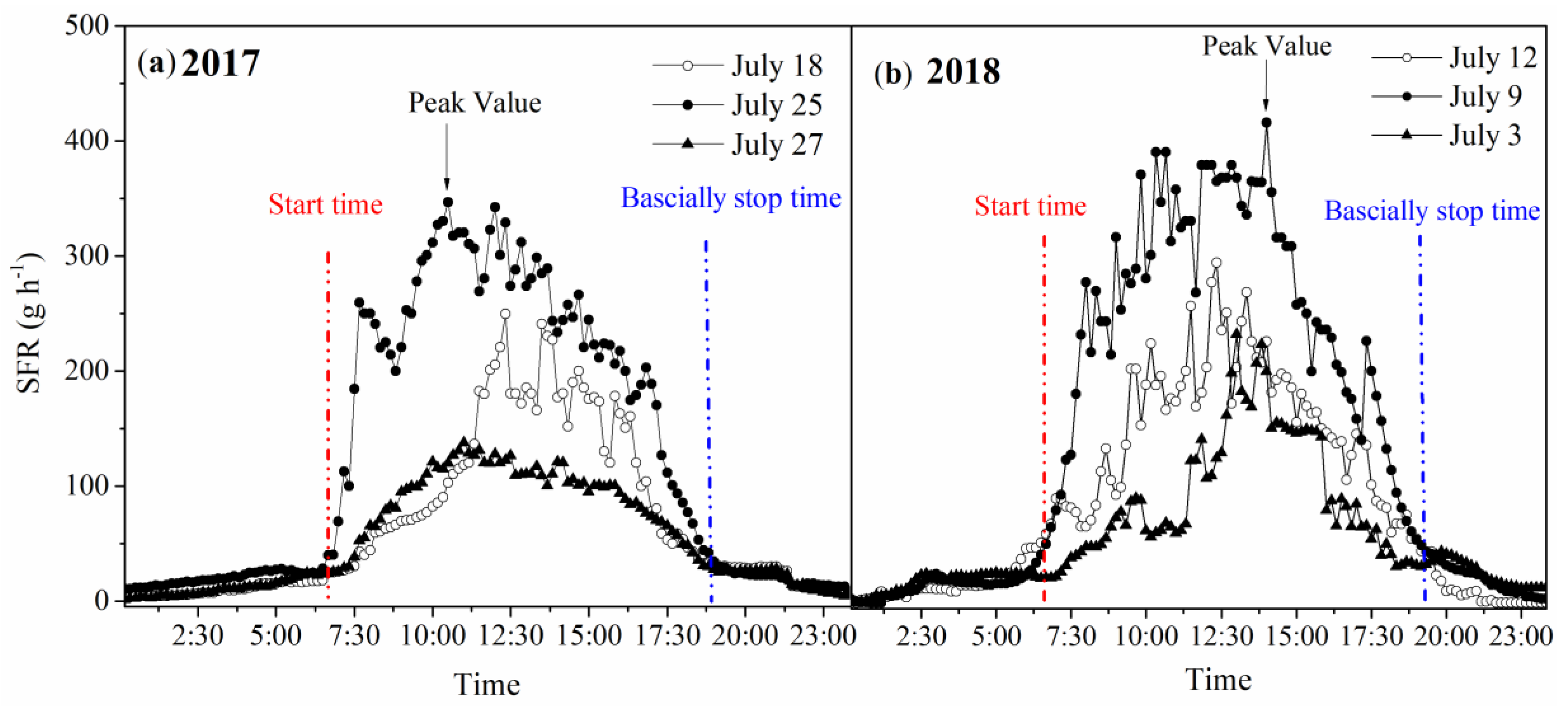
3.5. Diurnal Variations in SFR under Different Weather Conditions

The diurnal course of SFR under different typical days (sunny, cloudy, and rainy) is plotted in Figure 7. In order to avoid the obfuscation effect by plant vigor, typical days were selected in the same growing stage—27 July 2017 and 3 July 2018 were selected as typical rainy days (PAR = 8.38 and 9.54 mol m⁻² d⁻¹, respectively), 18 July 2017 and 12 July 2018 as typical cloudy days (PAR = 19.87 and 18.45 mol m⁻² d⁻¹, respectively), and 25 July 2017 and 9 July 2018 as typical sunny days (PAR = 37.78 and 40.12 mol m⁻² d⁻¹, respectively). In order to clearly describe the characteristics of the sap flow, three important time nodes (sap flow start time, stop time, and peak value) were selected for comparison. While on sunny days, the SFR followed unimodal peak dynamics, it followed multi-modal peaks dynamics on rainy and cloudy days. On sunny days, SFR rapidly increased to the peak value (SFR = 342.53 g h⁻¹ in 2017 and 390 g h⁻¹ in 2018) and the duration of vigorous sap flow lasted longer (about 6 h), giving rise to a conspicuously broad peak. Furthermore, the fluctuation in the SFR curve in peak times was stronger on sunny days. On rainy days, the SFR peak was attained 3 h later than on sunny days and with peak value lessened by 59.86% in 2017 and 62.4% in 2018, compared with sunny days. The peak value on rainy days occurred about 1.5 h ahead of that on cloudy days. On average, the SFR was, respectively, 122.85 and 143.08 g h⁻¹ in 2017 and 2018, on sunny days, which was significantly higher than that on cloudy (51.85 and 62.12 g h⁻¹) and rainy (42.08 and 42.25 g h⁻¹) days. There was little difference between the start and stop time of sap flow for the different typical days.

3.6. Lags and Hysteresis of Sap Flow

To further clarify diurnal variations in sap flow in grapevine in relation to the main climatic factors, diurnal hysteresis loops between SFR and PAR, and VPD and T are plotted in Figure 8. To further elucidate on how hysteresis varies with weather condition, different typical days—sunny day (PAR > 20 mol m⁻² d⁻¹), cloudy day (10 < PAR < 20 mol m⁻² d⁻¹) and rainy day (PAR < 10 mol m⁻² d⁻¹)—were separately analyzed. It was clear that time lags indeed existed. The change in SFR direction with PAR on a day was a counter-clockwise hysteresis, indicating that the variation in SFR lagged behind that of PAR in the day. On the contrary, clockwise hysteresis was observed in the day for a relationship between SFR and VPD and then between SFR and T. This showed that the variation in VPD and T with time during the day lagged behind that of SFR. The size of the hysteresis loop on cloudy and rainy days was obviously smaller than that on sunny days, but the direction of rotation was the same.

4. Discussion

4.1. Influence of Physiological Factors on Sap Flow

To date, the research carried out on the response of transpiration and physio-environmental factors of fruit trees has led to considerable advancement in our level of understanding of how its hydrological process is generated. In our study, we found that LAI = 2.5 m² m⁻² was the threshold of the LAI unsaturated stage and LAI saturated stage. The upper limit of LAI control on sap flow in the former stage indicated that transpiration capacity and potential increased with increasing LAI. Then, condition in the later stage suggested that transpiration capacity and potential did not increase further after LAI reached a certain degree. This was because transpiration water use largely relied on shortwave radiation: a pattern which was partly interpretable by Beer’s law [23]. In the LAI unsaturated stage, shortwave radiation intercepted by plant increases with the increase in leaf area, particularly when the radiation intensity was over or equal to the blade maximum intensity of light absorption. At this stage, the transpiration rate is proportional to the leaf area. With further increase in the LAI, leaves become overlapped, and short-wave radiation intercepted by leaves cannot continue to increase. Thus, the LAI determines the light interception capacity of the plant, thereby controlling the transpiration intensity.

On the contrary, other studies have reported different phenomena. For example, significant positive linear correlation was found between the LAI and sap flow at the rapidly increasing LAI stage, and no clear correlation was observed with the LAI due to the relative stability of the jujube plantation [21] and apple orchard [24]. This discrepancy could be attributed to the differences in the growing environments and species of the plants. The jujube and apple in the above studies were planted in Northwest China where there is severe dry climate and water scarcity. Therefore, water deficit was common in these orchards, particularly in the jujube plantations cultivated under rain-fed conditions. However, there was sufficient irrigation in the greenhouse experiment and the Aspen was grown in a sub-humid catchment [9]. Another possible reason was that different plant species have different physiological water use mechanisms in response to the environment.

4.2. Influence of Environmental Factors on Sap Flow

4.2.1. Daily Scale

Based on existing studies, the responses of sap flow to meteorological factors vary with the time scales [25]. On a daily scale, our result was in agreement with several studies [26,27], where both VPD and radiation were identified as important factors influencing transpiration. This is because VPD is indicated from the atmosphere water demand and radiation provides the energy for transpiration. Nonetheless, our results were different from those of Du et al. [28], where temperature and wind speed were identified as the main climate factors driving sap flow in the grapevine. Except for the differences in the sensitivities of plant cultivars to climatic factors, another explanation for the discrepancies in the results was that the environment was unique in our solar greenhouse where there were heat preservation measures and the micro-environment was isolated from the outside. This manmade condition caused relatively low temperature fluctuation and poor air circulation [29]. However, the grapevines in Du et al. [28] were planted in the desert oasis in Northwest China, where temperature difference was large and wind speed was strong. Under such conditions, it was no surprise that temperature and wind speed were not the main factors driving sap flow change in the grapevine in this study.

Numerous studies exploring the effects of soil moisture on plant water use note that the soil water processes affect transpiration activities, which are closely related with stomata regulation [30,31,32,33]. While obvious correlations have been noted between soil moisture and plant transpiration in a pool of other studies, no significant correlation was noted between SFR and SWC (R² = 0.01) in our study. This difference is mainly due to the different modes of water supply and the degree to which water demand was met. Many other experiments were conducted under water shortage conditions, as such, plant water use was evidently restricted by water availability. For example, low soil moisture considerably suppressed the transpiration of mature aspen and jack pine during the dry season in Canada [34]. Similarly, transpiration in the Mediterranean Quercus ilex forest decreased by 23% when precipitation soil moisture replenishment dropped by 29% in four successive years [35]. The canopy transpiration of Pinus laricio dropped by 50% when the only water source (rainfall) was avoided by using shelter in Southern Italy [36]. According to previous studies, ecosystem water use is largely limited by soil water availability in water-deficit regions, whatever the atmospheric demand [37,38,39,40,41,42,43,44,45,46,47,48,49]. Generally, soil moisture can affect plant water use when it is below a certain threshold. In our study, irrigation was controlled by root zone soil water content. For soil moisture lower than 70% of field water-holding capacity, irrigation automatically kicked in until soil moisture hit the upper limit of 90% field water-holding capacity. Our experiment was done under a no-water-shortage condition, hence no significant correlation between SFR and SWC was observed. Consistent with our study, O Brien [40] noted that soil water nearly had no impact on tree sap flow in wet tropical forests, and no clear correlation between soil moisture and sap flow was observed in Aspen in sub-humid zones with abundant precipitation [9]. Similar conclusions have been reached for various plant species and across multiple growth environments [41,42,43,44]. Although irrigation generally accounts for less than 10% of the total cost of cultivation under greenhouse conditions, it does not necessarily hold that the more irrigation supplied, the larger the yield, and the better the quality produced. Indeed, excess water can lead to excess environmental humidity that can further reduce fruit quality and increase diseases and pest attack [45]. Thus, appropriate irrigation control is required and should be emphasized in future studies.

There are also many studies on the accuracy comparison of integrated indicators and single indicators. According to Tie et al. [9], a simple linear equation between PAR × LAI and sap flow that does not consider other factors can be used to replace complex methods for transpiration estimation under negligible water stress condition, as it has a coefficient of determination as high as 0.89. Under similar no-water stress condition, the determination coefficient was 0.61 in our study, much lower than that recommended by the model reliability criterion (R² > 0.8) in other studies [46]. This suggests that there is a need for more accurate estimation of the micro-environments in greenhouse conditions.

4.2.2. Hourly Scale

For the correlation between the sap flow and meteorological factors at the hourly scale, we found that the overall trend in the different months was the same, except for August. This was attributed to the large water consumption by the grapevine in August, during which period both temperature and radiation were extremely high in the greenhouse. As grapevines maintain active transpiration to reduce greenhouse micro-temperature to avoid organ damage by heat stress [47], threshold control was not observed during this period, which was also supported by Figure 8. The above results agree with those in other studies with both linear and threshold responses of sap flow to the PAR [2,40,48,49]. However, plots of SFR against VPD or T roughly had the same parabolic curve. This stabilized with change in season, illustrating that VPD and T control on grapevine sap flow was relatively insensitive to seasonal change under greenhouse conditions. Besides, the correlations between hourly SFR and VPD, and T and RH were much weaker than that between hourly SFR and PAR for all the seasons. This was consistent with the daily trend, indicating that PAR was always the primary regulator of sap flow in grapevine under greenhouse condition.

4.3. Diurnal Variations of Sap Flow and Hysteresis Loops

In order to show diurnal variations in sap flow in grapevine in the study period and to limit uncertainty in the analysis [3], the diurnal variation in sap flow was analyzed using hourly average data. Shao et al. [50] reported unimodal peak and irregular multi-modal peak diurnal sap flow curves on sunny and rainy days, respectively. This was the same as the conclusion of our study. Compared with outdoor studies [7,20], the peak duration of sap flow was longer and the decline was slower in this study. This could be due to the slow drop in temperature in our greenhouse experiment where there was insulation effect. Additionally, SFR was near 0 (zero) early in the morning, but a little higher than 0 (zero) at night. This phenomenon could be caused by root pressure [4,51] that allows water to actively enter the plant during the night to supplement transpiration water loss at daytime, a process that in turn maintains plant water balance [52]. Night time sap flow has also been reported in many other studies. For example, Liu et al. [53] found that the amount of sap flow at nighttime accounted for 6% of daily transpiration in an intact forested watershed in South China.

A time lag between sap flow and climatic factors widely existed [40,54,55]. Our conclusion was much in agreement with that of O Grady et al. [7]. In contrast to previous reports [21,40], the increasing phase crossed with the decreasing phase of the hysteresis curve for SFR and PAR, whatever the weather was, in our study. This could be caused by the different patterns of change in climate. In our greenhouse, heat storage increased sharply with increasing radiation from morning to noon due to insulation effect, contributing to a faster rise in temperature than in outdoor conditions that, in turn, led to a further rapid rise in SFR. However, because of the same insulation effect, temperature dropped much slower in the greenhouse than outside under decreasing radiation from noon to night, leading to a slow decline in SFR. Consequently, there was an inverse change in the dynamics of SFR with PAR at different times of the day, resulting in the crossing hysteresis loops observed in this study. Compared with greenhouse conditions, the temperature increase and decrease variations at different times of the day are more consistent and parallel in field experiments [3], resulting in SFR and PAR hysteresis loops without obvious crosses.

5. Conclusions

Quite different from other studies conducted in outdoor condition, our study clearly clarified that the diurnal hysteresis curve between sap flow and radiation crossed regardless of weather, and weather condition altered the size, but not the direction, of the hysteresis loops. The new findings enhanced our understanding of the water use processes of greenhouse grapevine. Additionally, the environmental and physiological driving mechanisms of grapevine sap flow under solar greenhouse conditions in our study are useful for refining transpiration models and improving water use efficiency in the greenhouse environment.

References

1. Jasechko, S.; Sharp, Z.D.; Gibson, J.J.; Birks, S.J.; Yi, Y.; Fawcett, P.J. Terrestrial water fluxes dominated by transpiration. Nat. Cell Biol. 2013, 496, 347–350. [Google Scholar] [CrossRef] [PubMed]
2. Marques, T.V.; Mendes, K.; Mutti, P.; Medeiros, S.; Silva, L.; Perez-Marin, A.M.; Campos, S.; Lúcio, P.S.; Lima, K.; Dos Reis, J.; et al. Environmental and biophysical controls of evapotranspiration from Seasonally Dry Tropical Forests (Caatinga) in the Brazilian Semiarid. Agric. For. Meteorol. 2020, 287, 107957. [Google Scholar] [CrossRef]
3. Ma, C.; Luo, Y.; Shao, M.; Li, X.; Sun, L.; Jia, X. Environmental controls on sap flow in black locust forest in Loess Plateau, China. Sci. Rep. 2017, 7, 13160. [Google Scholar] [CrossRef] [PubMed] [Green Version]
4. Miner, G.L.; Ham, J.M.; Kluitenberg, G.J. A heat-pulse method for measuring sap flow in corn and sunflower using 3D-printed sensor bodies and low-cost electronics. Agric. For. Meteorol. 2017. [Google Scholar] [CrossRef]
5. Poyatos, R.; Villagarcía, L.; Domingo, F.; Piñol, J.; Llorens, P. Modelling evapotranspiration in a Scots pine stand under Mediterranean mountain climate using the GLUE methodology. Agric. For. Meteorol. 2007, 146, 13–28. [Google Scholar] [CrossRef]
6. Rana, G.; Ferrara, R.M.; Mazza, G. A model for estimating transpiration of rainfed urban trees in Mediterranean environment. Theor. Appl. Clim. 2019, 138, 683–699. [Google Scholar] [CrossRef]
7. O’Grady, A.P.; Worledge, D.; Battaglia, M. Constraints on transpiration of Eucalyptus globulus in southern Tasmania, Australia. Agric. For. Meteorol. 2008, 148, 453–465. [Google Scholar] [CrossRef]
8. Komatsu, H.; Kang, Y.; Kume, T.; Yoshifuji, N.; Hotta, N. Transpiration from aCryptomeria japonica plantation, part 1: Aerodynamic control of transpiration. Hydrol. Process. 2006, 20, 1309–1320. [Google Scholar] [CrossRef]
9. Tie, Q.; Hu, H.; Tian, F.; Guan, H.; Lin, H. Environmental and physiological controls on sap flow in a subhumid mountainous catchment in North China. Agric. For. Meteorol. 2017, 46–57. [Google Scholar] [CrossRef]
10. Macinnis-Ng, C.; Zeppel, M.; Palmer, A.; Eamus, D. Seasonal variations in tree water use and physiology correlate with soil salinity and soil water content in remnant woodlands on saline soils. J. Arid. Environ. 2016, 129, 102–110. [Google Scholar] [CrossRef]
11. Gong, X.; Liu, H.; Sun, J.; Gao, Y.; Zhang, H. Comparison of Shuttleworth-Wallace model and dual crop coefficient method for estimating evapotranspiration of tomato cultivated in a solar greenhouse. Agric. Water Manag. 2019, 217, 141–153. [Google Scholar] [CrossRef]
12. Yan, H.; Acquah, S.J.; Zhang, C.; Wang, G.; Huang, S.; Zhang, H.; Zhao, B.; Wu, H. Energy partitioning of greenhouse cucumber based on the application of Penman-Monteith and Bulk Transfer models. Agric. Water Manag. 2019, 217, 201–211. [Google Scholar] [CrossRef]
13. Rouphael, Y.; Colla, G. Modelling the transpiration of a greenhouse zucchini crop grown under a Mediterranean climate using the Penman-Monteith equation and its simplified version. Aust. J. Agric. Res. 2004, 55, 931. [Google Scholar] [CrossRef] [Green Version]
14. Ali, H.B.; Bournet, P.-E.; Cannavo, P.; Chantoiseau, E. Development of a CFD crop submodel for simulating microclimate and transpiration of ornamental plants grown in a greenhouse under water restriction. Comput. Electron. Agric. 2018, 149, 26–40. [Google Scholar] [CrossRef]
15. Van Herk, I.G.; Gower, S.T.; Bronson, D.R.; Tanner, M.S. Effects of climate warming on canopy water dynamics of a boreal black spruce plantation. Can. J. For. Res. 2011, 41, 217–227. [Google Scholar] [CrossRef]
16. Abdelfatah, A.; Aranda, X.; Savé, R.; De Herralde, F.; Biel, C. Evaluation of the response of maximum daily shrinkage in young cherry trees submitted to water stress cycles in a greenhouse. Agric. Water Manag. 2013, 118, 150–158. [Google Scholar] [CrossRef]
17. Alarcón, J.; Domingo, R.; Green, S.; Sánchez-Blanco, M.; Rodríguez, P.; Torrecillas, A. Sap flow as an indicator of transpiration and the water status of young apricot trees. Plant Soil 2000, 227, 77–85. [Google Scholar] [CrossRef]
18. Li, T.L. Science and Technology and Industrial Development Status and Trends of China’s Facilities Vegetable. China Rural Sci. Technol. 2016, 5, 77–79. [Google Scholar]
19. Shackel, K.A.; Johnson, R.S.; Medawar, C.K.; Phene, C.J. Substantial errors in estimates of sap flow using the heat balance technique on woody stems under field conditions. J. Am. Soc. Hortic. Sci. 1992, 117, 351–356. [Google Scholar] [CrossRef]
20. Solie, R.B.T.N. An Introduction to Environmental Biophysicsby Gaylon S. Campbell. Am. Sci. 1978, 66, 237–238. [Google Scholar] [CrossRef]
21. Chen, D.; Wang, Y.; Liu, S.; Wei, X.; Wang, X. Response of relative sap flow to meteorological factors under different soil moisture conditions in rainfed jujube (Ziziphus jujuba Mill.) plantations in semiarid Northwest China. Agric. Water Manag. 2014, 136, 23–33. [Google Scholar] [CrossRef]
22. Köstner, B.M.M.; Schulze, E.-D.; Kelliher, F.M.; Hollinger, D.Y.; Byers, J.N.; Hunt, J.E.; McSeveny, T.M.; Meserth, R.; Weir, P.L. Transpiration and canopy conductance in a pristine broad-leaved forest of Nothofagus: An analysis of xylem sap flow and eddy correlation measurements. Oecologia 1992, 91, 350–359. [Google Scholar] [CrossRef]
23. De León, M.A.P.; Bailey, B.N. Evaluating the use of Beer’s law for estimating light interception in canopy architectures with varying heterogeneity and anisotropy. Ecol. Model. 2019, 406, 133–143. [Google Scholar] [CrossRef] [Green Version]
24. Liu, C.; Du, T.; Li, F.; Kang, S.; Li, S.; Tong, L. Trunk sap flow characteristics during two growth stages of apple tree and its relationships with affecting factors in an arid region of northwest China. Agric. Water Manag. 2012, 104, 193–202. [Google Scholar] [CrossRef]
25. Kropp, H.; Loranty, M.M.; Alexander, H.D.; Berner, L.T.; Natali, S.M.; Spawn, S.A. Environmental constraints on transpiration and stomatal conductance in a Siberian Arctic boreal forest. J. Geophys. Res. Biogeosciences 2017, 122, 487–497. [Google Scholar] [CrossRef]
26. Massoud, E.C.; Purdy, A.; Christoffersen, B.; Santiago, L.; Xu, C. Bayesian inference of hydraulic properties in and around a white fir using a process-based ecohydrologic model. Environ. Model. Softw. 2019, 115, 76–85. [Google Scholar] [CrossRef] [Green Version]
27. Nagler, P.L.; Glenn, E.P.; Thompson, T.L. Comparison of transpiration rates among saltcedar, cottonwood and willow trees by sap flow and canopy temperature methods. Agric. For. Meteorol. 2003, 116, 73–89. [Google Scholar] [CrossRef]
28. Du, T.S.; Kang, S.Z.; Zhang, B.Z.; Li, S.E.; Yang, X.Y. Stem sap flow of grape under different drip irrigation patterns and its relationships with environmental factors in arid oasis region of Shiyang River basin. Chin. J. Appl. Ecol. 2008, 19, 299–305. [Google Scholar] [CrossRef]
29. Li, B.; Shi, B.; Yao, Z.; Shukla, M.K.; Du, T. Energy partitioning and microclimate of solar greenhouse under drip and furrow irrigation systems. Agric. Water Manag. 2020, 234, 106096. [Google Scholar] [CrossRef]
30. Duursma, R.A.; Blackman, C.J.; Lopéz, R.; Martin-StPaul, N.; Cochard, H.; Medlyn, B.E. On the minimum leaf conductance: Its role in models of plant water use, and ecological and environmental controls. New Phytol. 2018, 221, 693–705. [Google Scholar] [CrossRef] [Green Version]
31. Frank, D.C.; Poulter, B.; Saurer, M.; Esper, J.; Huntingford, C.; Helle, G.; Treydte, K.; Zimmermann, N.E.; Schleser, G.H.; Ahlström, A.; et al. Water-use efficiency and transpiration across European forests during the Anthropocene. Nat. Clim. Chang. 2015, 5, 579–583. [Google Scholar] [CrossRef] [Green Version]
32. Lin, Y.-S.; Medlyn, B.E.; Duursma, R.A.; Prentice, I.C.; Wang, H.; Baig, S.; Eamus, D.; De Dios, V.R.; Mitchell, P.J.; Ellsworth, D.S.; et al. Optimal stomatal behaviour around the world. Nat. Clim. Chang. 2015, 5, 459–464. [Google Scholar] [CrossRef] [Green Version]
33. E Ewers, B.; Gower, S.T.; Bond-Lamberty, B.; Wang, C.K. Effects of stand age and tree species on canopy transpiration and average stomatal conductance of boreal forests. Plant Cell Environ. 2005, 28, 660–678. [Google Scholar] [CrossRef]
34. Bernier, P.; Bartlett, P.; Black, T.; Barr, A.; Kljun, N.; McCaughey, J. Drought constraints on transpiration and canopy conductance in mature aspen and jack pine stands. Agric. For. Meteorol. 2006, 140, 64–78. [Google Scholar] [CrossRef]
35. Limousin, J.M.; Rambal, S.; Ourcival, J.M.; Rocheteau, A.; Joffre, R.; Rodriguezcortina, R. Long-term transpiration change with rainfall decline in a MediterraneanQuercus ilexforest. Glob. Chang. Biol. 2009, 15, 2163–2175. [Google Scholar] [CrossRef]
36. Cinnirella, S.; Magnani, F.; Saracino, A.; Borghetti, M. Response of a mature Pinus laricio plantation to a three-year restriction of water supply: Structural and functional acclimation to drought. Tree Physiol. 2002, 22, 21–30. [Google Scholar] [CrossRef] [PubMed]
37. Depante, M.; Morison, M.Q.; Petrone, R.M.; DeVito, K.J.; Kettridge, N.; Waddington, J.M. Hydraulic redistribution and hydrological controls on aspen transpiration and establishment in peatlands following wildfire. Hydrol. Process. 2019, 33, 2714–2728. [Google Scholar] [CrossRef]
38. Brown, S.M.; Petrone, R.M.; Chasmer, L.; Mendoza, C.A.; Lazerjan, M.S.; Landhäusser, S.M.; Silins, U.; Leach, J.; DeVito, K.J. Atmospheric and soil moisture controls on evapotranspiration from above and within a Western Boreal Plain aspen forest. Hydrol. Process. 2013, 28, 4449–4462. [Google Scholar] [CrossRef]
39. Mackay, D.S.; Ewers, B.E.; Cook, B.D.; Davis, K.J. Environmental drivers of evapotranspiration in a shrub wetland and an upland forest in northern Wisconsin. Water Resour. Res. 2007, 43. [Google Scholar] [CrossRef] [Green Version]
40. O’Brien, J.J.; Oberbauer, S.F.; Clark, D.B. Whole tree xylem sap flow responses to multiple environmental variables in a wet tropical forest. Plant Cell Environ. 2004, 27, 551–567. [Google Scholar] [CrossRef]
41. Wilson, T.G.; Kustas, W.; Alfieri, J.G.; Anderson, M.C.; Gao, F.; Prueger, J.H.; McKee, L.G.; Alsina, M.M.; Sanchez, L.A.; Alstad, K.P. Relationships between soil water content, evapotranspiration, and irrigation measurements in a California drip-irrigated Pinot noir vineyard. Agric. Water Manag. 2020, 237, 106186. [Google Scholar] [CrossRef]
42. Hölscher, D.; Koch, O.; Korn, S.; Leuschner, C. Sap flux of five co-occurring tree species in a temperate broad-leaved forest during seasonal soil drought. Trees 2005, 19, 628–637. [Google Scholar] [CrossRef]
43. Mutti, P.R.; Da Silva, L.L.; Medeiros, S.D.S.; Dubreuil, V.; Mendes, K.R.; Marques, T.V.; Lúcio, P.S.; e Silva, C.M.S.; Bezerra, B.G. Basin scale rainfall-evapotranspiration dynamics in a tropical semiarid environment during dry and wet years. Int. J. Appl. Earth Obs. Geoinf. 2019, 75, 29–43. [Google Scholar] [CrossRef]
44. Petousi, I.; Daskalakis, G.; Fountoulakis, M.; Lydakis, D.; Fletcher, L.; Stentiford, E.; Manios, T. Effects of treated wastewater irrigation on the establishment of young grapevines. Sci. Total. Environ. 2019, 658, 485–492. [Google Scholar] [CrossRef]
45. Girona, J.; Mata, M.; Arbonès, A.; Alegre, S.; Rufat, J.; Marsal, J. Peach Tree Response to Single and Combined Regulated Deficit Irrigation Regimes under Shallow Soils. J. Am. Soc. Hortic. Sci. 2003, 128, 432–440. [Google Scholar] [CrossRef] [Green Version]
46. Chen, D.; Wang, X.; Liu, S.; Wang, Y.; Gao, Z.; Zhang, L.; Wei, X.; Wei, X. Using Bayesian analysis to compare the performance of three evapotranspiration models for rainfed jujube (Ziziphus jujuba Mill.) plantations in the Loess Plateau. Agric. Water Manag. 2015, 159, 341–357. [Google Scholar] [CrossRef]
47. Neves, L.H.; Santos, R.I.N.; Teixeira, G.I.D.S.; De Araujo, D.G.; Silvestre, W.V.D.; Pinheiro, H.A. Leaf gas exchange, photochemical responses and oxidative damages in assai (Euterpe oleracea Mart.) seedlings subjected to high temperature stress. Sci. Hortic. 2019, 257, 257. [Google Scholar] [CrossRef]
48. Mendes, K.R.; Granja, J.A.A.; Ometto, J.; Antonino, A.C.D.; Menezes, R.S.C.; Pereira, E.C.; Pompelli, M.F. Croton blanchetianus modulates its morphophysiological responses to tolerate drought in a tropical dry forest. Funct. Plant Biol. 2017, 44, 1039. [Google Scholar] [CrossRef] [PubMed]
49. Dragoni, D.; Lakso, A.; Piccioni, R. Transpiration of apple trees in a humid climate using heat pulse sap flow gauges calibrated with whole-canopy gas exchange chambers. Agric. For. Meteorol. 2005, 130, 85–94. [Google Scholar] [CrossRef]
50. Shao, G.; Huang, D.; Cheng, X.; Cui, J.; Zhang, Z. Path analysis of sap flow of tomato under rain shelters in response to drought stress. Int. J. Agric. Biol. Eng. 2016, 9, 54–62. [Google Scholar] [CrossRef]
51. Chen, L.; Zhang, Z.; Li, Z.; Tang, J.; Caldwell, P.; Zhang, W. Biophysical control of whole tree transpiration under an urban environment in Northern China. J. Hydrol. 2011, 402, 388–400. [Google Scholar] [CrossRef]
52. Juhász, Á.; Sepsi, P.; Nagy, Z.; Tőkei, L.; Hrotkó, K. Water consumption of sweet cherry trees estimated by sap flow measurement. Sci. Hortic. 2013, 164, 41–49. [Google Scholar] [CrossRef]
53. Liu, X.; Li, Y.; Chen, X.; Zhou, G.; Cheng, J.; Zhang, D.; Meng, Z.; Zhang, Q. Partitioning evapotranspiration in an intact forested watershed in southern China. Ecohydrology 2014, 8, 1037–1047. [Google Scholar] [CrossRef]
54. Farrer, E.C.; Goldberg, D.E.; King, A.A. Time Lags and the Balance of Positive and Negative Interactions in Driving Grassland Community Dynamics. Am. Nat. 2010, 175, 160–173. [Google Scholar] [CrossRef]
55. Kume, T.; Komatsu, H.; Kuraji, K.; Suzuki, M. Less than 20-min time lags between transpiration and stem sap flow in emergent trees in a Bornean tropical rainforest. Agric. For. Meteorol. 2008, 148, 1181–1189. [Google Scholar] [CrossRef]
Figure 1. A map of Liaoning Province depicting the location of the site in the study area.
Water 12 03081 g001
Figure 2. Plots of temporal dynamics of leaf area index (LAI), photosynthetically active radiation (PAR), air temperature (T), vapor pressure deficit (VPD), variable of transpiration (VT), soil water content (SWC), relative humidity (RH) and daily transpiration (Tc) during the experimental period in 2017 (a1,b1,c1,d1,e1) and 2018 (a2,b2,c2,d2,e2).
Water 12 03081 g002
Figure 3. Plots of sap flow rate (SFR) responses to leaf area index (LAI) of grapevine grown in the greenhouse in 2017 and 2018 growing seasons in Northeast China.
Water 12 03081 g003
Figure 4. Plots of relationship between daily average sap flow rate (SFR) and six environmental factors—photosynthetically active radiation (PAR, (a)), vapor pressure deficit (VPD, (b)), variable transpiration (VT, (c)), air temperature (T, (d)), soil water content (SWC, (e)) and relative humidity (RH, (f)) in 2017 and 2018 experimental periods.
Water 12 03081 g004
Figure 5. Relationship between daily sap flow rate (SFR) and three integrated indexes—photosynthetically active radiation by leaf area index (PAR × LAI, (a)), vapor pressure deficit by leaf area index (VPD × LAI, (b)) and variable transpiration by leaf area index (VT × LAI, (c))—in 2017 and 2018 experimental periods.
Water 12 03081 g005
Figure 6. Plots of relationship between hourly sap flow rate (SFR) and environmental factors—(a) photosynthetically active radiation (PAR), (b) vapor pressure deficit (VPD), (c) air temperature (T) and (d) relative humidity (RH) in different months in 2018. Note that the red line is the regression relationship for data in August, and the black line is that for data in other months.
Water 12 03081 g006
Figure 7. Daily changes in grapevine sap flow rate (SFR) under different weather conditions during the 2017 (a) and 2018 (b) experimental periods.
Water 12 03081 g007
Figure 8. Changes in daily cycle of hourly mean sap flow rate (SFR) for (a) photosynthetically active radiation (PAR), (b) air temperature (T) and (c) vapor pressure deficit (VPD) in a day, for sunny (PAR > 20 mol m−2 d−1, (a1,b1,c1)), cloudy (10 mol m−2 d−1 < PAR< 20 mol m−2 d−1, (a2,b2,c2)), and rainy (PAR < 10 mol m−2 d−1, (a3,b3,c3)) days in 2017 and 2018 experimental periods. Note that arrow denotes direction of change with time and n denotes number of days with corresponding typical climatic conditions.
Water 12 03081 g008