Numerical Simulation of Free Surface Flow on Spillways and Channel Chutes with Wall and Step Abutments by Coupling Turbulence and Air Entrainment Models

Abstract

Spillways and channel chutes are widely used in hydraulic works. Two kinds of abutment—walls and steps—are usually constructed to dissipate energy; however, they may also cause cavitation at the abutment position. In this study, we used Flow 3D with the Reynolds-averaged Navier–Stokes (RANS) and large eddy simulation (LES) turbulent models which included air entrainment to simulate the free surface flow through the spillway, channel chute and stilling basin of the Ngan Truoi construction to optimize the configuration of walls and dams. We measured the water level, velocity and pressure to estimate the influence of grid size and the turbulent model type used. Our results highlight the need to include air entrainment in the model simulating rapid flow over a hydraulic construction. With adjustments for energy loss, this study shows that walls provide the best results and the optimal distance between two walls is 2.8 m.

1. Introduction

The safety of dams and other hydraulic works (e.g., spillways, sluice gates, stilling basins) plays an important role in water resources management in many countries because its failure can cause disasters downstream. Therefore, studying the hydraulic characteristics of flow over constructions with different working conditions is always considered an important task. Computational fluid dynamic (CFD) simulation is an effective and robust tool with which to simulate many complicated hydraulic phenomena. Demeke [1] selected the Flow 3D model to calculate flow over spillways and channels. Salmasi [2] utilized both the Ansys Fluent model and experiments to study flow over a stepped spillway. The commercial Flow 3D model based on Navier–Stokes equations has been applied frequently to address many environmental issues. This software provides various modules, such as viscosity and turbulence, air entrainment, shallow water and granular flow, to solve complicated hydraulic problems including supercritical flow, shock wave due to dam break flow, hydraulic jump in stilling basin, etc. Studies on the hydraulic characteristics of stepped spillways have been widely researched [3,4,5,6,7,8,9,10]. “White flow” can be observed when a rapid velocity flow occurs on a channel chute and stilling basin due to self-aeration and turbulent features. Several studies have used a coupling of turbulence and air entrainment modules within Flow 3D to verify the effectiveness and robustness of this model. Valero [10] calibrated an air entrainment module in CFD spillway applications. Arnau [11] performed an assessment of OpenFoam and Flow 3D in the numerical modeling of a low Reynolds number hydraulic jump. Valerio [12] reviewed several studies of water and gas flow and divided spillways into two types—smooth and step slope spillways. Bore [13] indicated that a step spillway and chute can yield negative pressure and increase the cavitation potential at the steps. However, step spillways are less prone to cavitation erosion than smooth ones. Although Felder and Chanson [14] provided some conclusions of energy loss with mild-sloped channel chutes, to the best of our knowledge, the hydraulic profile of free surface flows on channel chutes with a small slope and regularly distributed abutments have not been studied in depth using an air–water numerical model. In Vietnam, this kind of channel chute is quite common—there are more than 50 such constructions and their slope varies from 5% to 15%, with length ranging from 50 m to 250 m depending on the surrounding topography. In extreme cases, a large input unit discharge induces very high velocity in the channel. Therefore, in order to dissipate energy in the channel chute, as well as reduce the dimensions of the stilling basin, the optimal abutment types in the channel chute should be considered. Besides the advantages of abutments, they also generate vacuum pressure, which increases the risk of cavitation, [15]. Hence, besides estimating the energy dissipation of the two types of abutment considered here—wall (W) and step (S)—evaluating their cavitation potential is also important.

In this paper, we used the commercial software Flow 3D with the Reynolds-averaged Navier–Stokes (RANS) and Large Eddy Simulation (LES) turbulent models, the volume of fluid (VOF) method, and the sub grid model for air entrainment, density evaluation and drift-flux to study the two phases of water–gas flow over the spillway and channel chute with two types of abutment. A case study from Ngan Truoi, Ha Tinh province was used in the physical model introduced in [16], and was selected for analysis here. The simulated velocity, water level profile and pressure data were are compared with measured data. The location of the submerged hydraulic jump in the stilling basin and the pressure profile on several steps connecting the channel chute and stilling basin are also indicated. We also used our analysis to determine the optimal distance between abutments.

2. Materials and Methods

2.1. Air Entrainment and Turbulent Models in Flow 3D

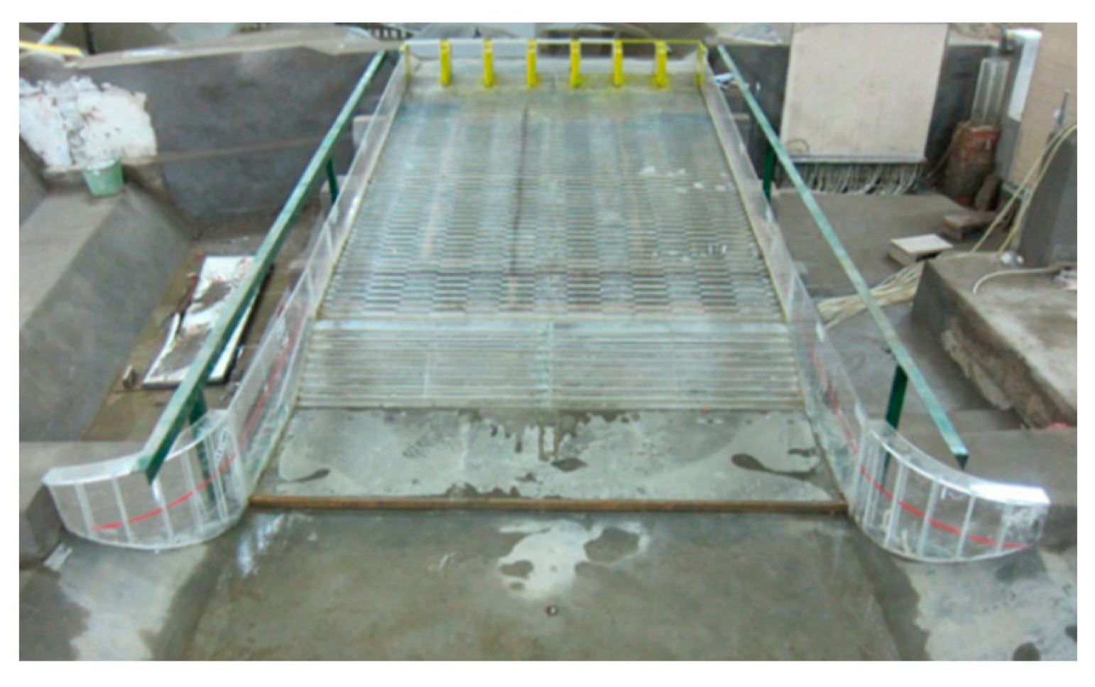
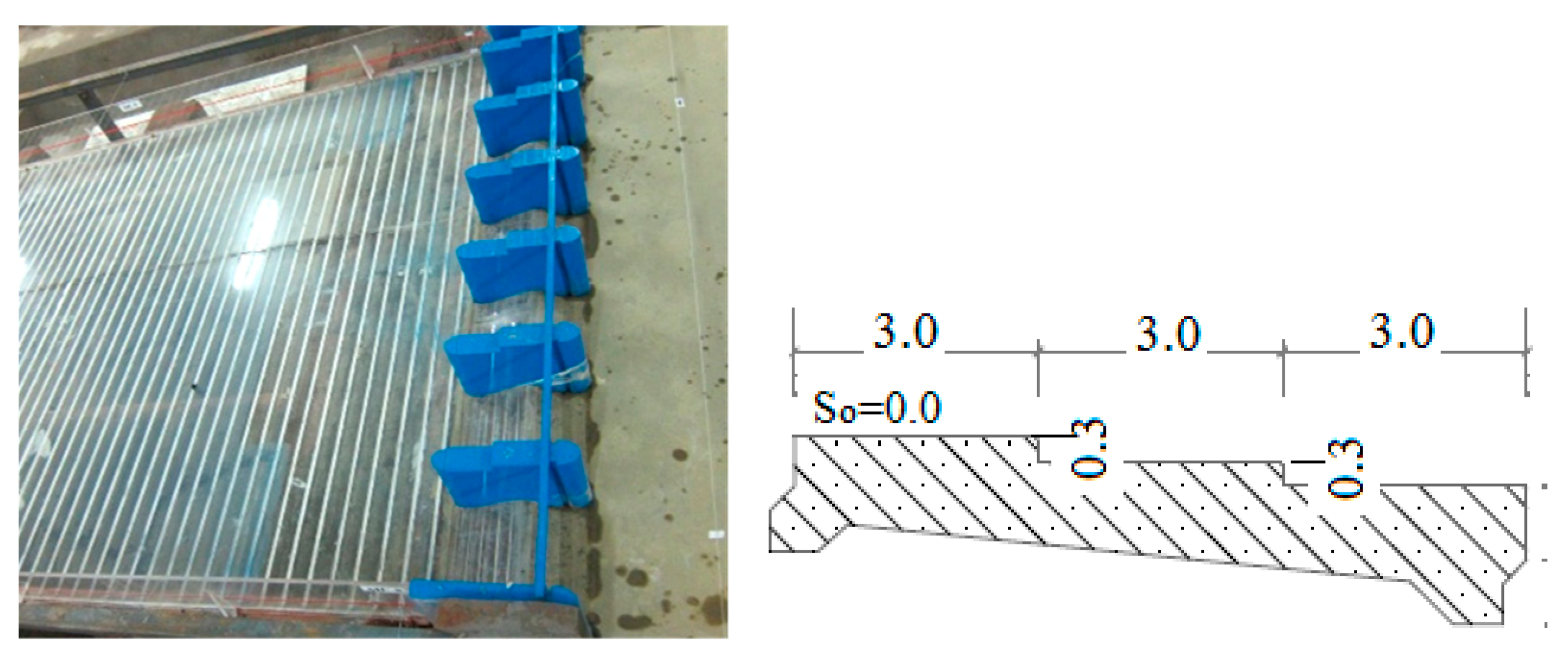
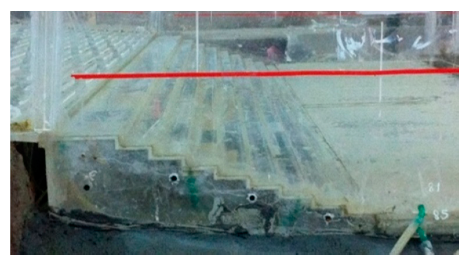
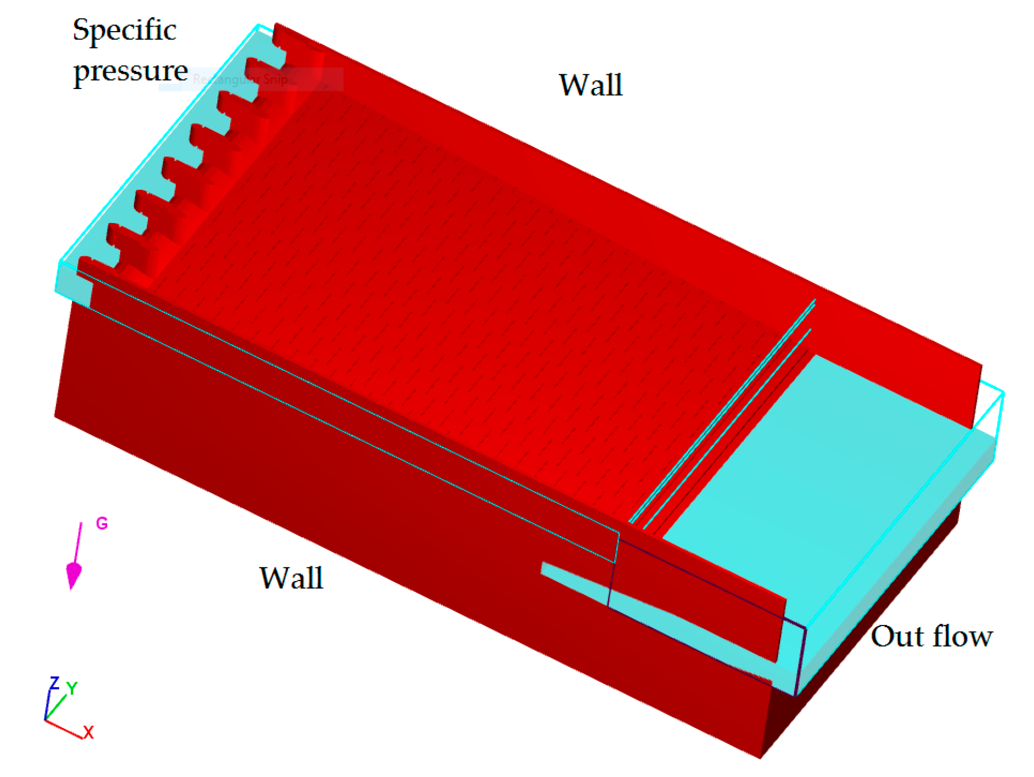
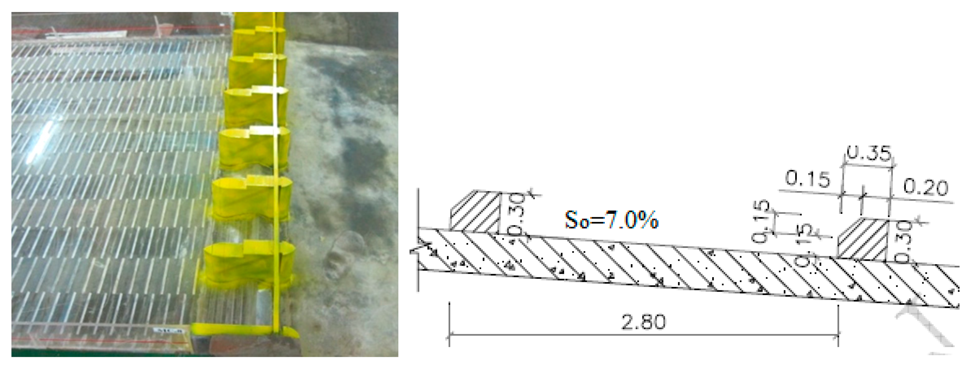
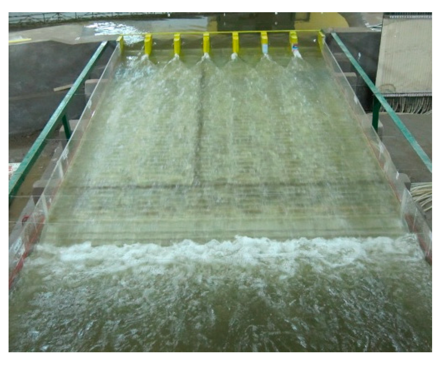
The commercial CFD software Flow 3D version 12 was used to simulate the hydraulic characteristics of complex problems. Flow 3D is based on the VOF method to solve the system equation of mass and momentum conservation laws, while Navier–Stokes equations and the TurVOF method are used for interface tracking [17]. In version 12, Flow 3D replaced the simplest volume-based air entrainment model option with the existing mass-based model. The mass-based model is more physics-based since, unlike volume, entrained air mass is conserved, while its volume changes in response to the surrounding fluid pressure. In the case of self-aeration, the entrainment of gas can be modeled by the air entrainment model. The air entrainment model estimates the rate at which gas (represented by void regions) is entrained into the flow using a balance of stabilizing forces (gravity and surface tension) and destabilizing forces (turbulence) [18]. For air–water flow, the density is not constant. Thus, the continuity formula is written as

$$\frac{\partial {\rho }_a}{\partial t}+\nabla \times \left({\rho }_{a}u\right)-\nabla \times \left(\upsilon \nabla {\rho }_a\right)=0$$

(1)

where ρ_a is the volume minus the weighted average density and u is velocity.

The momentum equation of air entrainment flow is expressed by

$$\frac{\partial \left({\rho }_a{u}_a\right)}{\partial t}+\nabla \times \left({\rho }_a{u}_a{u}_a\right)=-\nabla P+{\rho }_{a}g+\nabla \times \tau =0$$

(2)

where P is pressure, τ is Reynolds stress tensor and g is gravity acceleration.

The air entrainment model in Flow 3D offers the option to include buoyancy and bulking in the output, meaning that areas of variable density flows can be accurately represented. This model can capture air going into the surface of a rapid flow when the flow is turbulent. Buoyancy effects can be included by selecting the “activate bulking” and “activate buoyancy” options and defining the associated parameters. For the activate bulking option, the density evaluation model accounts for non-uniform fluid density by using the value for density of phase#2 in the model panel. The activate buoyancy option enables the drift flux model to estimate the interaction between the two phases. The air bubble can enter the fluid due to the difference in their densities and affects the fluid’s motion. The drift flux model requires the “viscous flow” option be enabled.

When modeling turbulent flows, Flow 3D recommends using Reynolds-averaged Navier–Stokes (RANS) with the two equations k-ε (RNG), or the two equations k-ω. Previous studies [6,9] suggest that the RNG turbulence model is the most accurate when simulating turbulent rapid flow on a group of structures, so we selected it to compute all flow characteristics in this research.

The LES model is beneficial when dealing with problems associated with small spartial scale constructions. In terms of air–water flow, Lubin [19] used this model to study the air bubble occurring in plunging breaking waves. However, there are no examples of using the LES model for free surface flow over a complex group of structures. In this paper, we use both turbulent models to simulate the two-phase liquid–gas flow over a complex structure.

2.2. Physical Model

The project “Design Ngan Truoi- Ha Tinh hydraulic construction” was established by Vietnam Hydraulic Engineering Consultants Corporation (HEC). The physical model was constructed at Key Laboratory of River and Coastal Engineering with a ratio of 1/50 to examine the outflow capacity; water level; velocity; and pressure profiles on the weir and spillway chute; and to estimate the energy dissipation of two abutment types (wall and step) corresponding to the different operational working conditions (Figure 1). The 7-gate weir had a width of 12 m per gate, and a height of 3.4 m; this was followed by a rectangular channel chute with a slope gradient of 7%, 140 m in length and 108 m in width. There are two kinds of abutment: step and wall were constructed regularly along channel chute on laboratory to investigate and compare its advantage and disadvantage in hydraulically point of view, (see Figure 2 and Figure 3). Peak elevations of pier and weir are +57.80 m and +48.60 m, respectively. The 9-step segment connected between channel chute and stilling basin is 23 m long. Its elevation varied from +30 m to +30.64 m, so the height of each step is 0.75 m. The stilling basin has 108 m of width, 30 m of length and bed elevation is +30 m. The gauges are set up at center line of hydraulic work to collect hydraulic data. Two types of abutment were constructed (steps and walls), corresponding with two scenarios, that is, the design case and complete case, respectively. The details of the two scenarios can be seen in Figure 3 and Figure 4, and are demonstrated in [16]. At the end of the channel chute, a stepped segment was constructed to connect the chute with the stilling basin (Figure 4). The measured data from the physical model were multiplied by the physical scale to obtain values for the original design; then, we compared these data with the solution of the model. The two tests we selected to make this comparison are indicated on

Table 1. Working conditions.

No	Flow Rate Q (m3/s)	Upstream Water Level Zup (m)	Downstream Water Level Zdown (m)
1	3319	55.86	39.54
2	1061	52.00	35.11

.

The commercial sofware Flow 3D verson 12 was utilized to study flow over the group of hydraulic structures (spillway, channel chute, stilling basin) in a protoplast of the Ngan Truoi hydraulic construction. AutoCAD-3D was used to draw and generate a stereolithographic (stl) file to use in Flow 3D as a solid boundary.

The computational model with a width of 108 m and length of 215 m was divided to two blocks (Figure 5). Block 1 consisted of the spillway and channel chute. Block 2 contained a stepped segment and the stilling basin. The boundary in flow direction of block 1 was X_min (specific pressure), corresponding with the upstream water elevation; the boundary of X_max was symmetric. For block 2, the boundary of X_max was flow out. Both boundaries of the Y direction are the wall, while in the lower Z direction the boundaries are the wall and the upper boundary is specified pressure with fluid fraction is set equal to zero. The Manning coefficient n was set to 0.017. The initial conditions were water elevations both upstream and downstream corresponding with different operating conditions, as shown in Table 1. The numerical solution was obtained with different mesh resolutions (1.0 m, 0.75 m, 0.5 m) for all domains, consisting of 463,500, 1,098,666, and 3,708,000 cells, respectively. The finest mesh size of 0.1 m was also used with the Y axis of 1.0 m width, with 4,500,000 cells in total to simulate hydraulic characteristic in the stilling basin.

3. Result and Discussion

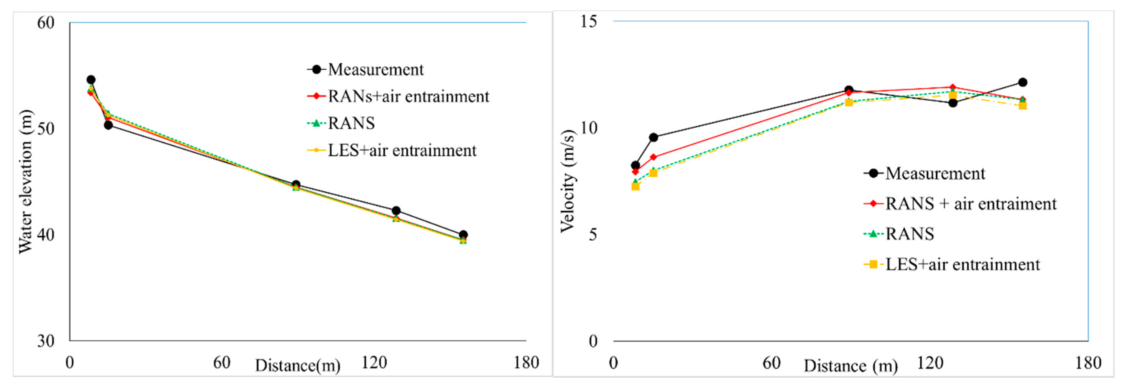
3.1. The Influence of the Turbulence Model

Two turbulence models were constructed on Flow 3D software: RANS-Renormalized Group (RNG) and LES were implemented to research a range of hydraulic feartures on the spillway, chute and stilling basin and determine the effect of abutments in the design and complete case scenarios presented here. A cell size of 0.1 m was used in this study. The relative error quantity (R) was calculated by

$$R_i=\frac{X_{meas,i}-X_{sim,i}}{X_{meas,i}}·100$$

(3)

where X_sim is the simulated value, X_meas is the measured data and i is the index of the gauge’s order.

Table 2. Water elevation and velocity in case 1.

No	X (m)	Zbed (m)	Water Level					Velocity
			Zmeas (m)	ZRANs (m)	RZ,RAN (%)	ZLES (m)	RZ,LESs (%)	Vmeas (m/s)	VRANs (m/s)	RV,RAN (%)	VLES (m/s)	RV,LES (%)
7	8.30	48.60	54.62	53.40	2.23	53.76	1.57	8.25	7.94	3.74	7.24	12.74
8	15.13	46.40	50.35	51.07	−1.42	51.27	−1.83	9.56	8.62	9.82	7.89	19.42
9	89.23	41.10	44.73	44.49	0.54	44.38	0.79	11.77	11.65	1.05	11.19	4.97
10	128.63	38.30	42.30	41.57	1.71	41.43	2.06	11.17	11.90	−6.55	11.53	−3.05
11	155.13	36.40	40.00	39.51	1.21	39.40	1.50	12.14	11.33	6.69	11.03	9.77

shows the numerical results obtained from the two turbulent models in case 1 of Table 1. These datsa were then compared with the observed data of water elevation and velocity profiles.

In general, the mathematical solutions for both cases match well with experimental ones in all gauges. The velocity was over-estimated, expecially at point 8, when the effect of piers on free surface flow is quite strong. Besides, the relative error (R) of numerical results obtained by the RANS model is higher than that obtained by the LES model. This is because the LES model should be applied for domains with a very fine mesh. The water level was modeled more accurately than the velocity, that is, its R value is smaller.

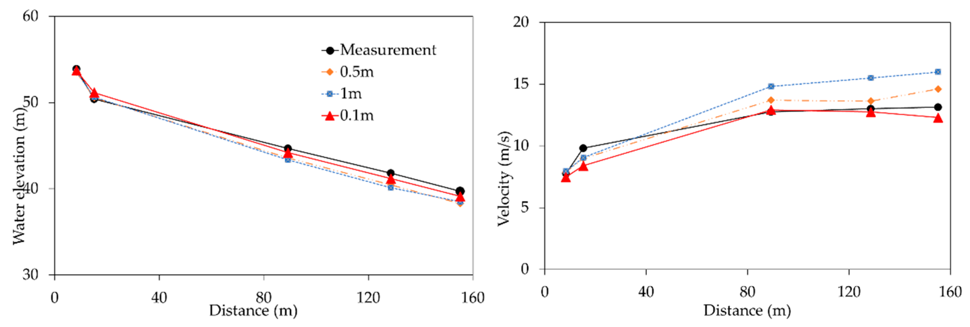
3.2. The Influence of Discretization Schemes

To evaluate the impact of grid size in generating numerical solution, 4 cell sizes, namely, 1.0 m, 0.75 m, 0.5 m, 0.1 m were selected to get water elevation (Z) and depth averaged velocity (V) at 5 gauses on the centerline of spillway and chute. In this section, RANs equation was used to estimate hydraulic characteristics. The accuracy of numerical result is estimated by Nash-Sufficent number. This parameter is defined by the following formular:

$$Nash=1-\frac{{\displaystyle \sum _{i=1}^N{\left(X_{sim,i}-X_{obs,i}\right)}^2}}{{\displaystyle \sum _{i=1}^N{\left(X_{obs,i}-{\overline{X}}_{obs}\right)}^2}}$$

(4)

where X_sim and X_obs are predicted and observed values of water elevation and velocity; i is index of gauges; N is total of gauges.

The Nash values of Z and V are shown in

Table 3. Nash coefficient of water level.

Zup (m)	Grid Size (m)
	1.00		0.75		0.50		0.10
	Design	Complete	Design	Complete	Design	Complete	Design	Complete
55.86	0.95	0.93	0.96	0.93	0.96	0.93	0.98	0.98
52.00			0.97	0.96		0.96	0.97	0.99

and

Table 4. Nash coefficient of velocity.

Zup (m)	Grid Size (m)
	1.00		0.75		0.50		0.10
	Design	Complete	Design	Complete	Design	Complete	Design	Complete
55.86	0.17	0.22	0.79	0.68	0.82	0.71	0.85	0.79
52.00			0.75	0.65		0.66	0.81	0.71

. Nash coefficient of water level was approximately 1.0 for all cell sizes. However, in Table 4, the Nash coefficient of velocity was very low for the coarsest mesh size (1 m). A grid size of 0.5 m or 0.75 m yielded acceptable hydraulic data, so, they could be used for the whole domain. The design case gave better results than the complete case. The higher the input water level is, the better the hydraulic solution becomes; this is because a steady flow over the hydraulic structure with distributed abutments can be maintained easily. Figure 6 shows more detail of the Z and V values at five study points in the mathematical and physical models of the design case. There is good agreeement between the numerical solution with a cell size of 0.1 m and the empirical solution. Ther FAVOR^TM tool in Flow 3D provides a discretization of the solid boundary with two resolutions (0.75 m and 0.1 m), which means the obstacles are almost removed (Figure 7). Therefore, the numerical solution can not be influenced by the walls or steps.

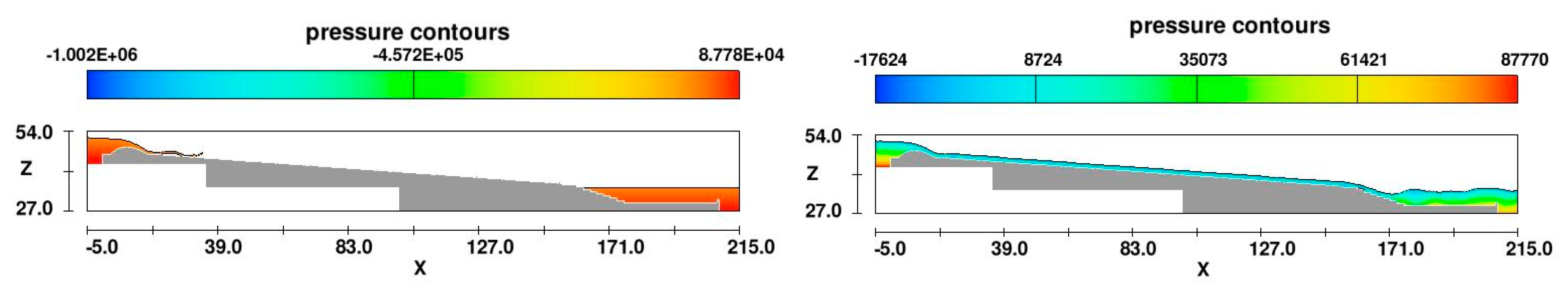
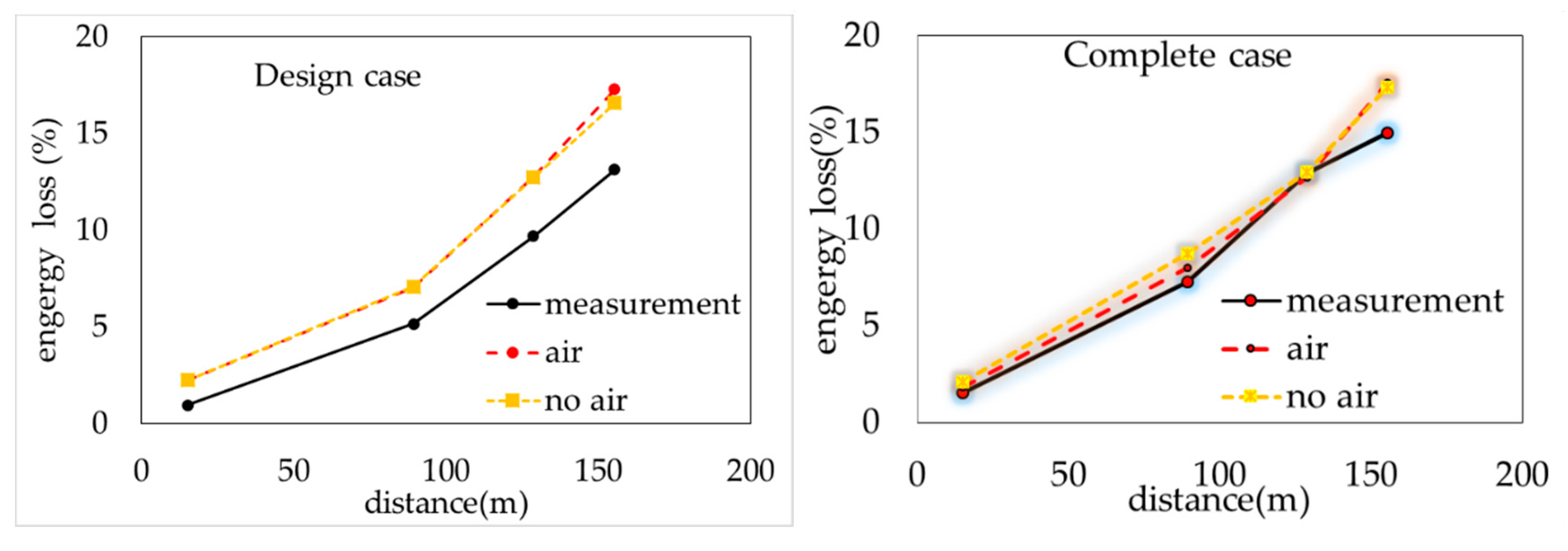
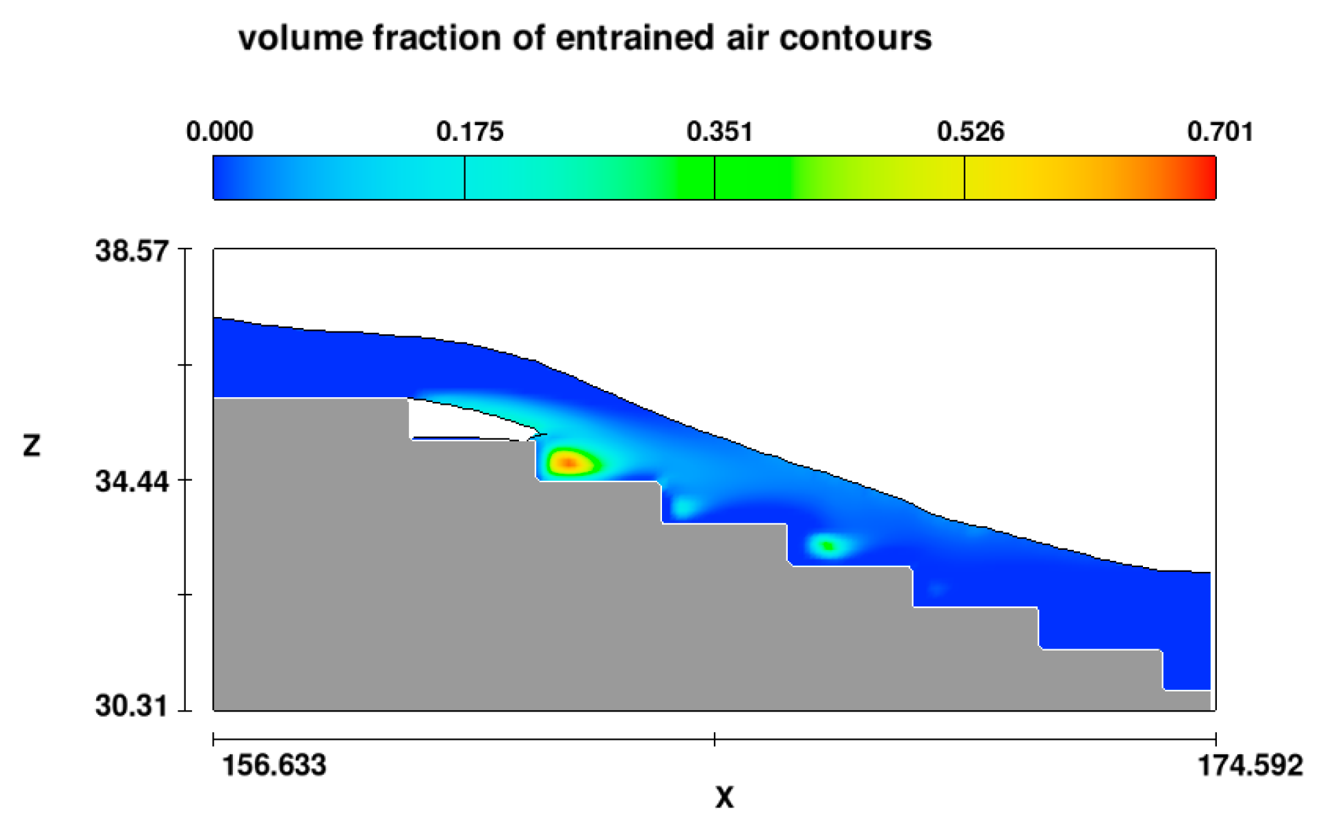
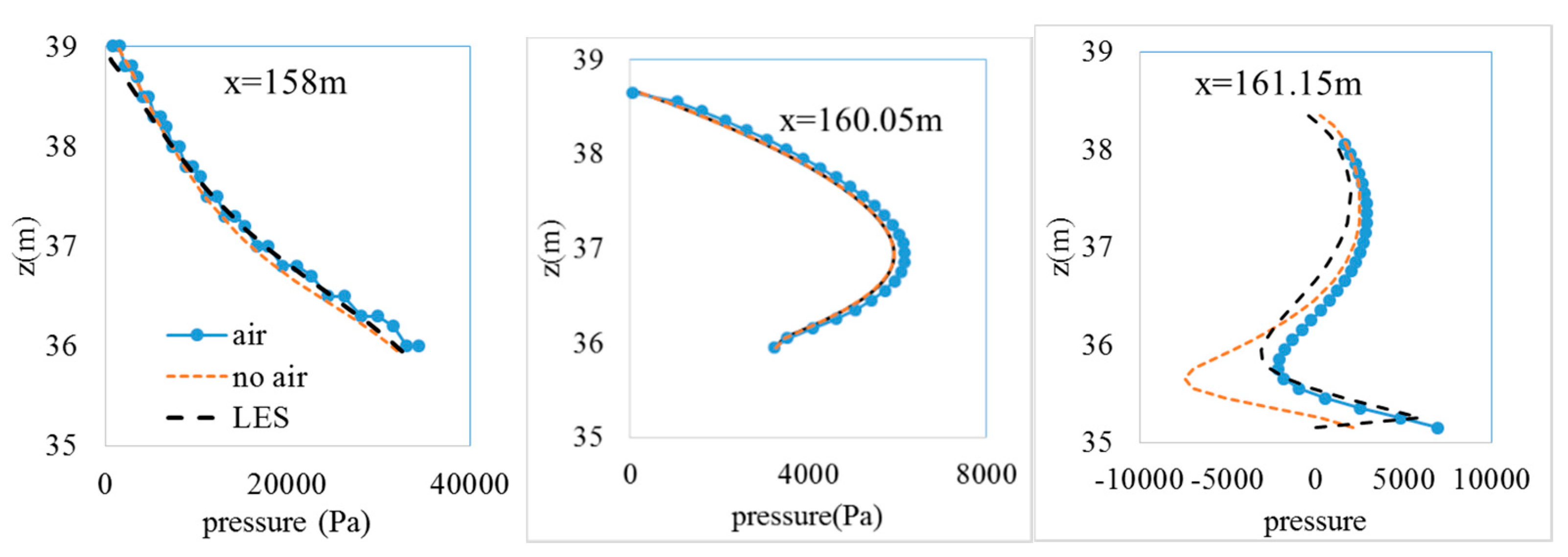
3.3. The Influnce of the Air Entrainment Model on Mathematical Results

For small discharges, the flow regime is a napped flow. An increase of discharge may induce the appearance of a skimming flow regime [14]. Two-phase water–gas flow appears on a set of hydraulic structures. Due to the existence of many abutments on the channel chute, the flow is turbulent and gas easily enters the napped flow when the input discharge reduces. Figure 8 demonstrates two numerical results obtained with and without the air entrainment model when measuring this type of flow. Regardless of air entraiment, the jet flow goes far from the obstacle, so it does not exist in the real case.

Additionally, Figure 9 shows that when the input water level is low (Z_up = 52 m), the free surface flow on the spillway chute can be only simulated by Flow 3D with both the tuburlence and air entrainment modules. If the entrainment module is not actived, the software Flow 3D does not work after 20 m length of spillway and chute. This point can be explained by Figure 10, which indicates percentage of air in the water flow calculted by the air entraiment model. At the cross section at 20 m, this ratio is approximately equal to zero, while at the locations 50 m, 100 m and 150 m along the spillway and chute, the maximum values of the void fraction are 0.5%, 0.35%, 0.32%, respectively, when the obstacle is a wall, and 0.01%, 0.1%, 0.2%, respectively, when the obstacle is a step. Hence, regardless of the air entrainment module, the simulation is not acceptable.

The water elevation and velocity were measured using five guages, and one phase water and two phase water–gas flow data were compared with the measured data (Figure 11). There is no significant difference between the water levels calculated by both scenarios, except at the second gauge, where the flow is strongly fluctuated because of the oblique waves after piers. The velocity results measured by the RANS model and air entrainment model are closest to the empirical solution, except in the case of gauge 4. At gauge 3, the relative error yeilded by RANS and air entraintment models was 0.83% in comparison with 4.5% of the result calculated by only turbulent one.

3.4. Esimate Flow Characteristics on Stirlling Basin

Under the second working conditions (Z_up = 52 m) with the physical model, the vacumn pressure was observed on the second and the third step of the segment between the chute and stilling basin. In the design project, this value varied from 2648 Pa to 3924 Pa, but it is smaller, at around 590 Pa, in the complete case [16].

Table 5. Maximum numerical vacumn pressure on step segment.

No	Zup (m)	Max Pvac (Pa) - Design Case	Max Pvac (Pa) - Complete Case
1	55.86	23,561.5	9027.2
2	52.00	4549.5 (2nd step); 6242.8 (3rd step)	894.9 (2nd step); 981.2 (3rd step)

presents the numerical solution of vacumn pressure taken from steps in both the design and complete cases. In the Flow 3D solution, the influence of the gas phase on flow is clearly seen via the volume fraction air parameter (Figure 12). The jet of bubble air appears after the second step because in the first step there is a blank space on the face. Thus, air bubbles enter the lowrer and upper layers of a free surface flow.

Three different numerical models—RANS turbulence model with the air entrainment model (a) and without the air entrainment model (b); and the LES turbulence model with the entrained air model (c)—were used to calculate the pressure profiles at three points on the first step of the complete case. At the beginning and middle of the second step’s face, the profiles of the three cases are quite similar. However, at the tip of this step, case (b) majorly overestimates when the minimum pressure is equal to –6000 Pa. Therefore, it does not provide a good fit with the measured data (Figure 13).

The phenomenon of submerged hydraulic jumps in the stilling basin occurred under all operating conditions of the physical model (see Figure 14 and Figure 15). This feature was reproduced by coupling the turbulence model RANS-RNG and the air entraiment model. There was an acceptable level of agreement between the calculated and measured data regarding the hydraulic jump’s location (

Table 6. Location of hydraulic jump.

Zup (m)	Design Project		Complete Project
	Physical	Mathematical	Physical	Mathematical
55.86	Middle of 4th step	End of 4th step	Begin of 4th step	End of 4th step
52.00	End of 5th step	Begin of 6th step	Begin of 6th step	Middle of 6th step

).

The distribution of pressure calculated by the three different models at the middle of the stilling basin (x = 192.05m) was similar, except for case (c), which gave negative values near the surface of the flow. Furthermore, the profile of u-velocity in the x direction showed strong fluctations. The maximum negative and positive values were around 10 m/s. A vortex appeared when two backward flowpaths occurred at the bottom and the surface of the flow in the basin. The w-velocity direction was downwards in all three cases and the maximum value of 3 m/s was obtained by model (a), (Figure 16).

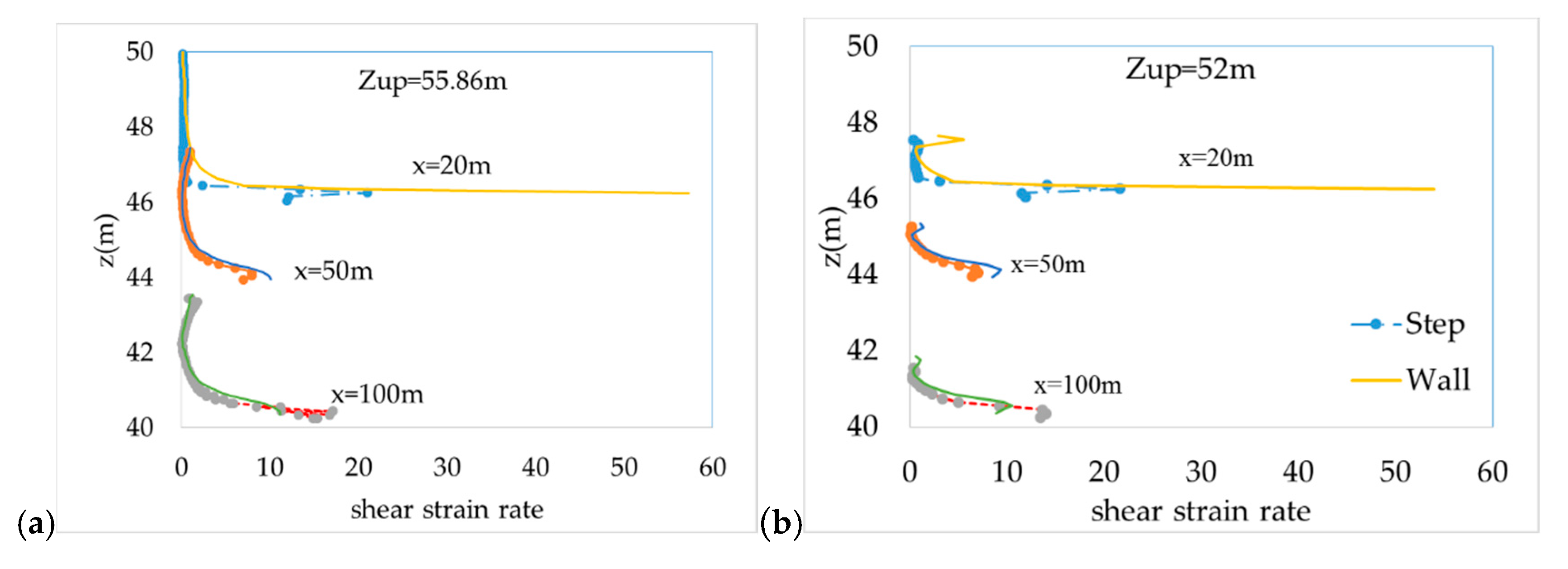
3.5. Estimated Energy Dissipation Capability of Two Types of Abutment

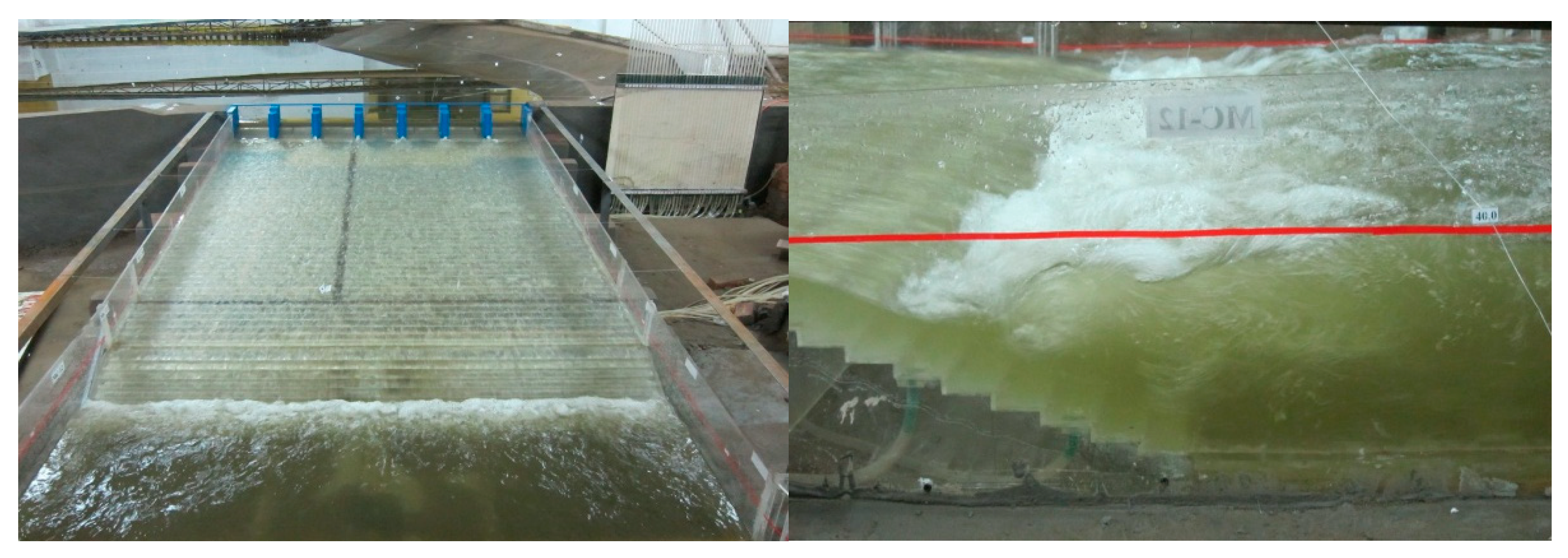
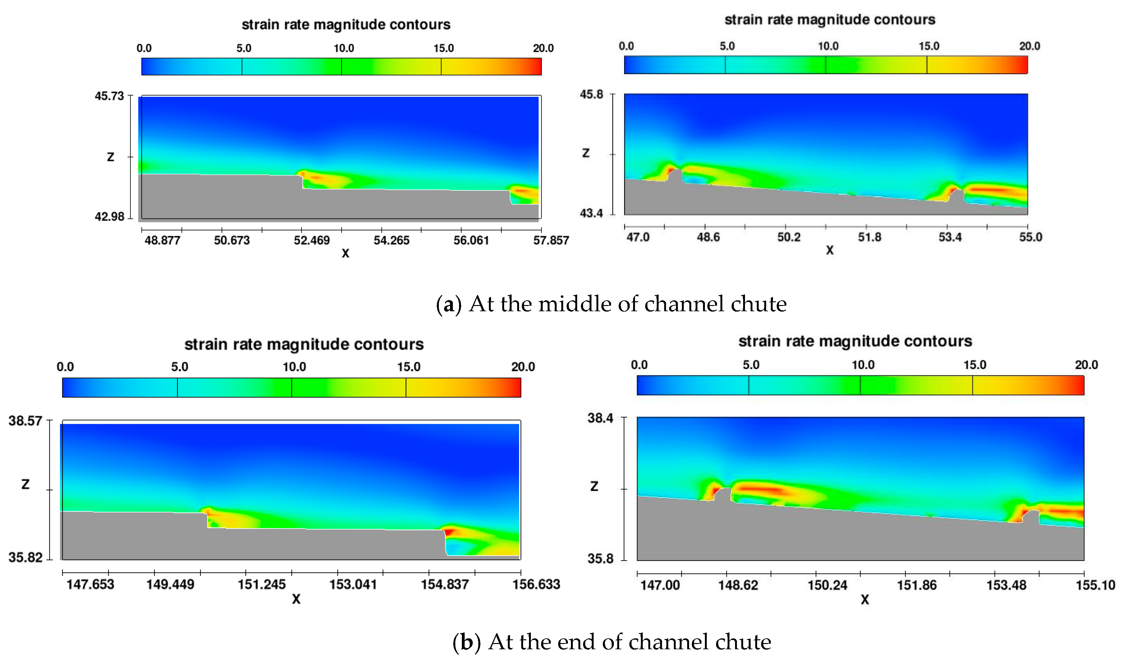
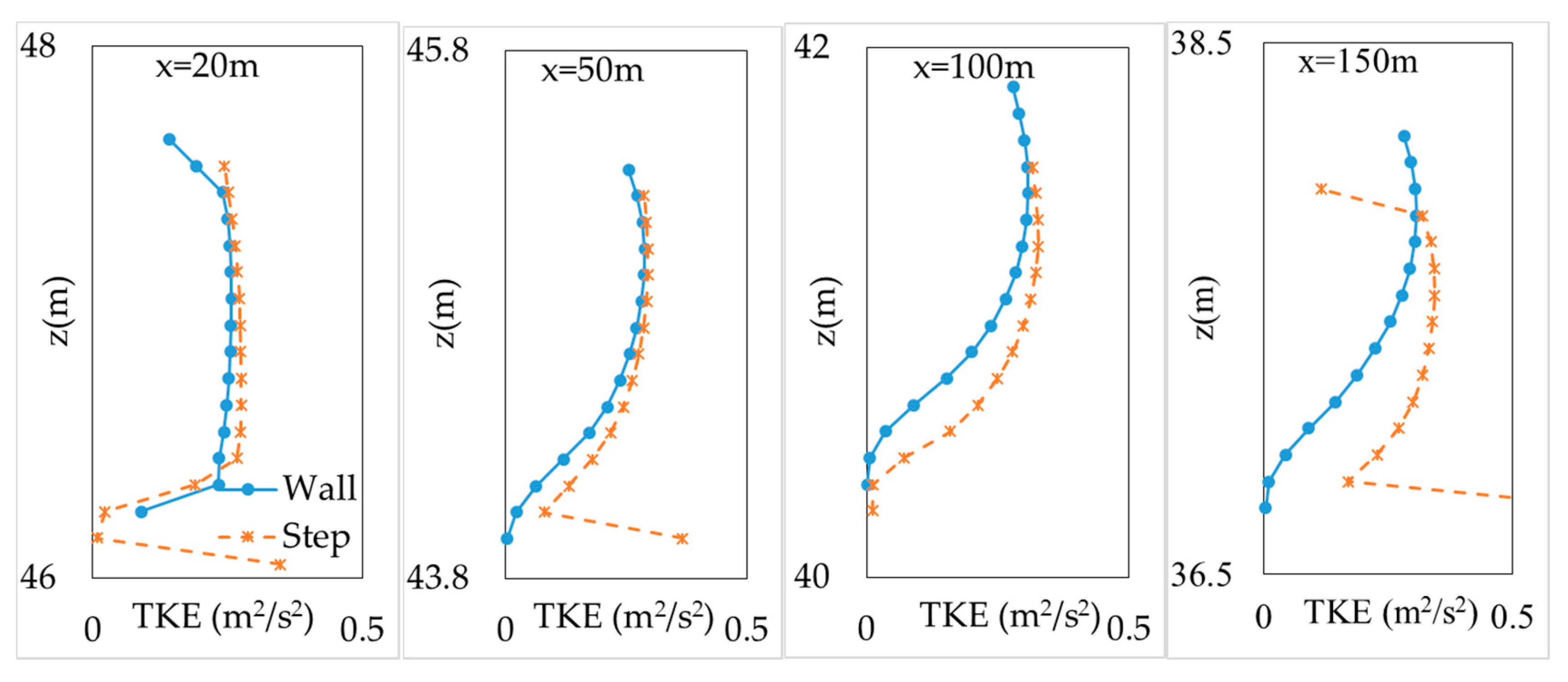
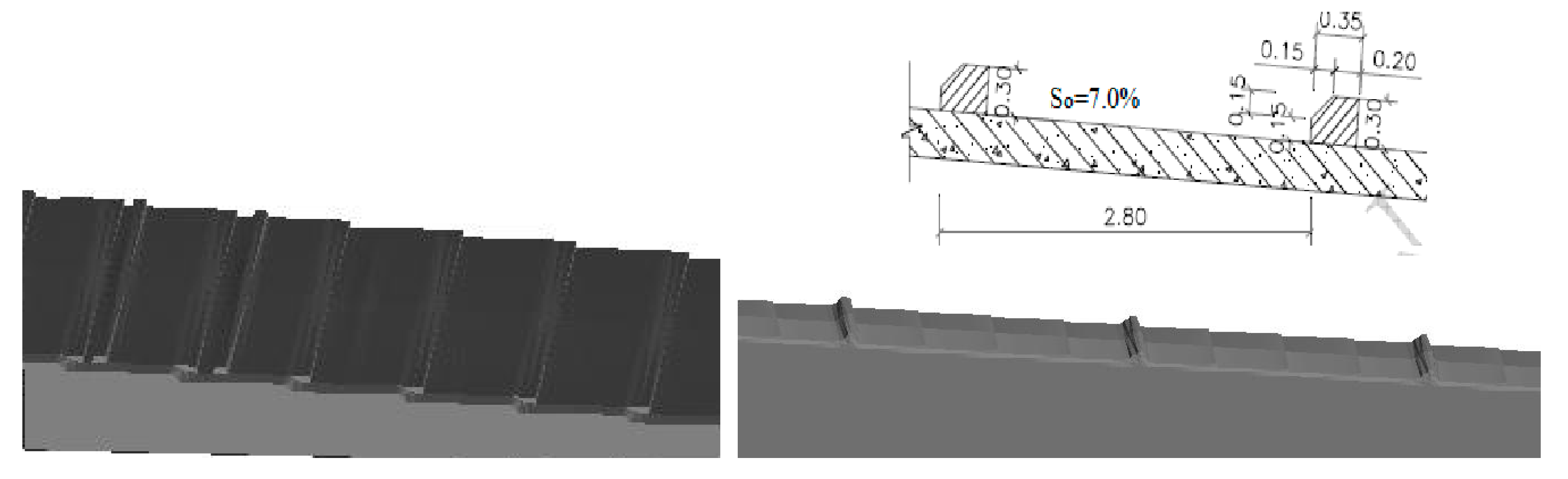
3.5.1. Hydraulic Characteristics of the Channel Chute with Wall Abutments

Abutments distributed regulary along the channel chute can reduce flow energy dramatically. According to Chanson [15], when the volume flow rate reduces, a napped flow can occur. In addition, a high intensity shear layer develops near the bottom of the bed, which is an important feature impacting energy dissipation. It also generates vacuum pressure in the channel chute. High shear stress regions can cause vortexes and second flows behind abutments. The pressure at its center reduces and can lead to negative pressure at the abutment. Figure 17 indicates the distribution of the shear strain rate magnitude obtained by Flow 3D. The red areas, demonstrating the maximum strain rate magnitude, which occurred after steps were smaller than those occurring after walls.

Figure 18 shows that the wall abutment develops a larger shear stress layer. The significant difference is seen at the thickness of 0.4 m–0.8 m from the bottom of the bed. This point can be explained by the results shown in Figure 19, which displays the distribution of u-velocity on the z axis at different positions. This value near the bottom of the wall abutment is smaller than the value at the bottom of the step abutment. Therefore, the turbulence kinetic energy (TKE) at these locations exhibted a similar trend (Figure 20). The u-velocity and TKE obtained by numerical models for the shear stress layer were similar with or without the air entrainment model. However, at the end of the channel chute, the flow velocity near the bottom of the wall abutment was 3–5 m/s lower than for the step abutment. In the half of flow depth above, the velocity trend for the two abutment types is identical, so the variation of TKE is similar as well.

In the case of a lower input water level, the displacement between two TKE profiles is greatest (Figure 21). This finding is related to the development of a roughness layer: The smaller the thickness of the TKE layer, the greater the turbulence length scale is.

In a skimming flow regime, the steps cause more friction and a larger roughness layer. Most of the engergy is dissipated to maintain stable vortices beneath the pseudo-bottom formed by the external edges of the steps. The vortices are maintained through the transmission of turbulent shear stress between the skimming stream and the recirculating fluid underneath. According to Chanson [15], energy loss in an ungated spillway and channel chute can be estimated by Equation (5):

$$\frac{\Delta H}{H_{\max }}=1-\frac{{\left(\frac{f}{8·\sin \alpha }\right)}^{1/3}·\cos \alpha +\frac{1}{2}·{\left(\frac{f}{8·\sin \alpha }\right)}^{-2/3}}{\frac{2}{3}+\frac{H_{dam}}{d_c}}$$

(5)

where f is the friction factor, α is the channel slope, H_dam is the dam head crest above the downstream toe and H₀ is the free surface elevation above the spillway crest. For an ungated spillway, the maximum head available and the dam height are determined by H_max = H_dam + 1.5.d_c, where d_c is the critical depth.

The percentage of energy loss under both working conditions in Table 1, calculated by Equation (5), was 17.7% and 21.9%, respectively. Note that Equation (5) in this analysis neglects the effect of air entraiment.

The expression generally adopted to estimate energy dissipation along the spillway and chute is written by

$$h_L{}_i={\left(Z_u+\frac{V_u^2}{2g}\right)}_i-{\left(Z_d+\frac{V_d^2}{2g}\right)}_i$$

(6)

where Z_u, V_u and Z_d, V_d are the water level and depth-average velocity at upstream and downstream cross sections of a segment, respectively.

In the case of the highest input water level (Z_up = 55.86 m), the volume flow rate reached up to 3319 m³/s, and energy loss was determined along spillway and chute with both the design and complete cases by numerical and physical models. As can be seen from Figure 22, the observed data show that energy loss at the end of the chute of the design project was 13.12%, which was smaller than the complete case, with 14.94 %. Similarly, the percentage of this term calculated by Flow 3D showed the same trend (17.23% for the design case compared with 17.55% for the complete case). Besides that, the depth of the average velocity magnitude along the channel chute with the step abutment was higher than that with the wall one (see Figure 22). These points show that, from a hydraulic perspective, the complete project gives better results than the design case.

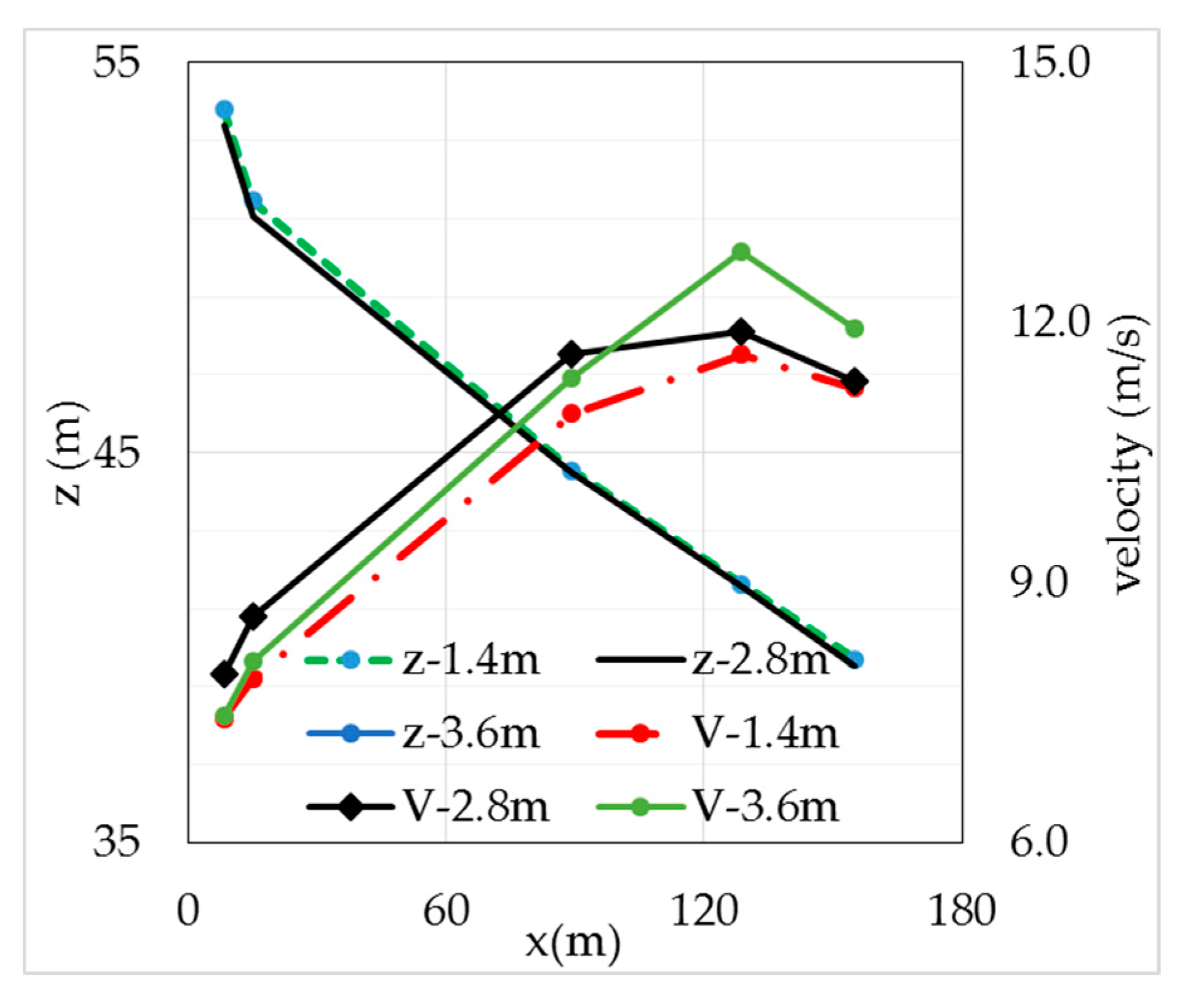
3.5.2. Optimal Distance between Two Walls

Morris [20] indicated that the most effective distance between two obstacles (l) is in the range (7.5–12 d), where d is the height of the wall, so that a shock wave fully depvelops within this distance. In this research, d = 0.3 m, so we study the capability of distance engery loss in the first operating working condition when l was taken as three different values—1.4 m, 2.8 m and 3.6 m—by the Flow 3D model.

When the concentration of wall abutment distribution is higher (l = 1.4 m) or lower (l = 3.6 m) than the original design (l = 2.8 m), the water level along the channel chute varies slightly (Figure 23). Most of the difference between the three cases of distance was observed in the velocity. When l = 1.4 m, the velocity at all five gauges was smaller than at l = 2.8 m. At a distance of x = 15.13 m after the spillway and x = 89.23 m, the difference in velocity was 8.3% and 5.9%, respectively. When the abutments are distributed further apart (l = 3.6m), the velocity at the beginning of the chute is higher than with the original design, although it is lower at the end of the chute.

The percentage energy loss (ΔE/E) yielded by the three abutment distances (1.4 m, 2.8 m, 3.6 m), as estimated by Equation (6) is shown in

Table 7. Energy loss.

l (m)	1.4	2.8	3.6
ΔE/E(%)	17.36	17.55	16.92

, where E is total head at upstream of spillway. As the maximum value was obtained with an abutment distance of 2.8 m, this was deemed the optimal distance between abutments to maximize energy dissipation. Although the distance 1.4 m gives a lower velocity and head loss is slightly smaller than the 2.8 m spacing, the price of the former is more costly because the number of abutments required increases. Moreover, the numerical solution shows that there is no submerged jump in the stilling basin if a spacing distance of 1.4 m is used. Therefore, the complete project with a 2.8 m spacing between wall abutments distributed regularly along the channel chute is the optimal configuration from a hydraulic perspective.

4. Conclusions

In this research, various hydraulic characteristics (water depth, velocity, pressure profiles, energy loss) of the Ngan Truoi hydraulic works with two abutment types (walls and steps) were investigated using both numerical and physical models. We have reached the following conclusions:

• Two turbulent models (RANS and LES) were used to calculate features. The results showed that RANS gives better solutions for the water level, velocity and pressure profiles.
• Four discretization types (1 m, 0.75 m, 0.5 m and 0.1 m) were used. The finest mesh cell of 0.1 m yeilded the best match between numerical model results and the physical measurements.
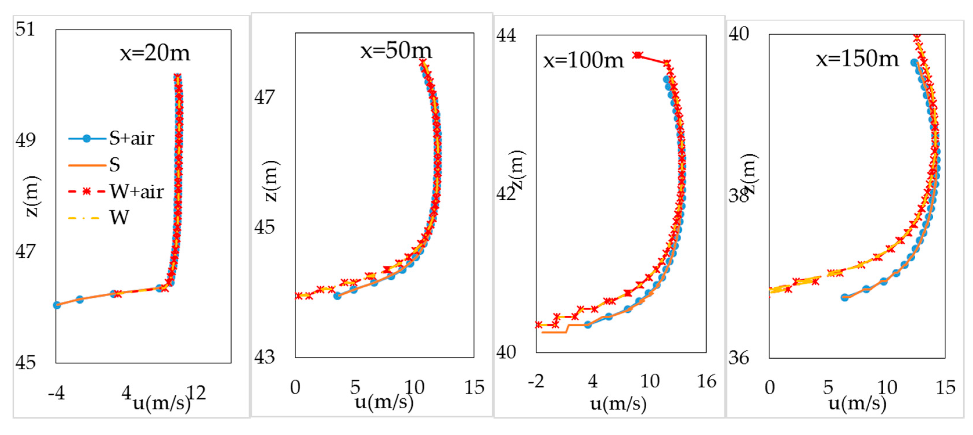
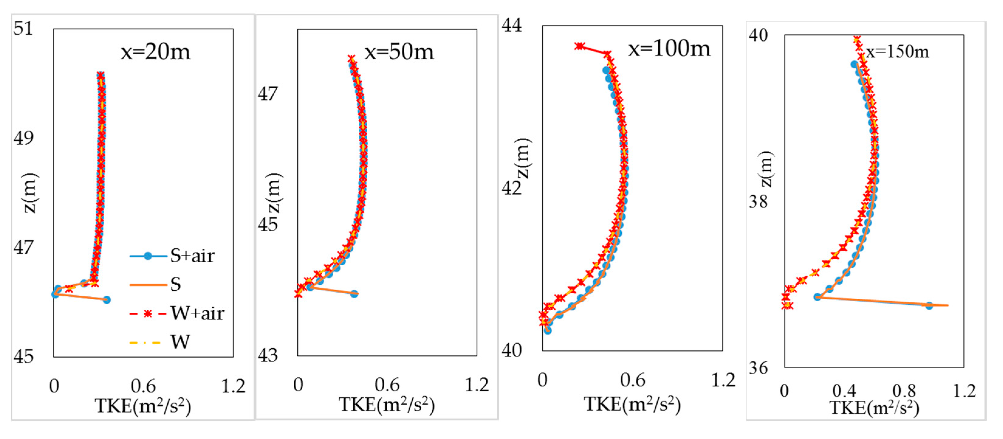
• An air entrainment model was included to simulate rapid flow over a complex structure. The predictions for the water level, velocity in the spillway chute, pressure distribution, and the location of the hydraulic jump in the stilling basin all closely agreed with measured data. The study also indicates that, without the air entrainment model, air–water flow cannot be simulated well if the water input is low and a napped flow occurs.
• The estimation of engergy dissipation also indicates that wall abutments provide better energy dissipation. The maximum strain rate after steps was smaller than after walls. Three spacing distances between abutments were tested on the spillway chute to study energy dissipation along the chute. Our results showed that the distance of 2.8 m dissipated energy better than other spacings.

References

1. Demeke, G.K.; Asfaw, D.H.; Shiferaw, Y.S. 3D Hydrodynamic Modelling Enhances the Design of Tendaho Dam Spillway, Ethiopia. Water 2019, 11, 82. [Google Scholar] [CrossRef] [Green Version]
2. Salmasi, F.; Samadi, A. Experimental and numerical simulation of flow over stepped spillways. Appl. Water Sci. 2018. [Google Scholar] [CrossRef] [Green Version]
3. Amador, A.; Juny, M.S.; Dolz, J. Developing flow region and pressure fluctuations on steeply sloping stepped spillways. J. Hydraul. Eng. 2009, 135, 1092–1100. [Google Scholar] [CrossRef]
4. Bayon, A.; Toro, J.P.; Bombardelli, F.A.; Matos, J.; Lospez-Jiménez, P.A. Influence of VOF technique, turbulence model and discretization scheme on the numerical simulation of the non-aerated, skimming flow in stepped spillways. J. Hydro Environ. Res. 2018, 19, 137–149. [Google Scholar] [CrossRef] [Green Version]
5. Dong, Z.; Wang, J.; Vetsch, D.F.; Boes, R.M.; Tan, G. Numerical simulation of air water two phase flow on stepped spillway behind X shaped flaring gate piers under very high unit discharge. Water 2019, 11, 1956. [Google Scholar] [CrossRef] [Green Version]
6. Bombardelli, F.A.; Meireles, I.; Matos, J. Laboratory measurements and multi-block numerical simulations of the mean flow and turbulence in the non-aerated skimming flow region of steep stepped spillways. Environ. Fluid Mech. 2011, 11, 263–288. [Google Scholar] [CrossRef] [Green Version]
7. Morovati, K.; Eghbalzadeh, A. Study of inception point, void fraction and pressure over pooled stepped spillways using Flow-3D. Int. J. Numer. Methods Heat Fluid Flow 2018, 28, 982–998. [Google Scholar] [CrossRef]
8. Kermani, E.F.; Barani, G.A. Numerical simulation of flow over spillway based on CFD method. Sci. Iran. A 2014, 21, 91–97. [Google Scholar]
9. Kumcu, S.Y. Investigation of flow over spillway modeling and comparison between experimental data and CFD analysis. KSCE J. Civ. Eng. 2017, 21, 994–1003. [Google Scholar] [CrossRef]
10. Valero, D.; Rafael, G.B. Calibration of an Air Entrainment Model for CFD Spillway Applications. Adv. Hydroinform. 2016, 38, 571–582. [Google Scholar] [CrossRef]
11. Arnau, B.; Daniel, V.; Rafael, G.B.; Francisco, J.V.M.; Amparo, L.J. Performance assessment of OpenFOAM and FLOW-3D in the numerical modeling of a low Reynolds number hydraulic jump. Env. Model. Softw. 2016, 80, 322–335. [Google Scholar]
12. Valerio, D. On the Fluid Mechanics of Self-Areation in Open Channel Flow. Ph.D. Thesis, Liege University, Liege, Belgium, November 2018. [Google Scholar]
13. Bore, R.M. Guidelined on the design and hydraulic characteristics on stepped spillways. In Proceedings of the 24th ICOLD Congress, Kyoto, Japan, 6–8 June 2012; pp. 203–220. [Google Scholar]
14. Felder, S.; Chanson, H. Energy dissipation, flow resistance and gas-liquid interfacial area in skimming flows on moderate-slope stepped spillways. Environ. Fluid Mech. 2009, 9, 427–441. [Google Scholar] [CrossRef]
15. Chanson, H. Comparison of energy dissipation between nappe and skimming flow regimes on stepped chutes. J. Hydraul. Res. 1994, 32, 213–219. [Google Scholar] [CrossRef]
16. Key Laboratory of River and Coastal Engineering. Báo cáo kết quả thí Nghiệm mô hình Thủy Lực—Tràn xả lũ Ngàn Trươi PA6B; Key Laboratory of River and Coastal Engineering: Hanoi, Vietnam, 2008. (In Vietnamese) [Google Scholar]
17. Flow Science Inc. Flow-3D, Version 12.0; User Mannual; Flow Science Inc.: Santa Fe, NM, USA, 2020. [Google Scholar]
18. Hint, C.W. Modeling Turbulent Entrainment of Air at a Free Surface; Technical Note FSI-01-12; Flow Science, Inc.: Santa Fe, NM, USA, 2003. [Google Scholar]
19. Lubin, P.; Vincent, S.; Abadie, S.; Caltagirone, J.P. Three dimensional large eddy simulation of air entrainment under plunging breaking waves. Coast. Eng. 2006, 53, 631–655. [Google Scholar] [CrossRef] [Green Version]
20. Morris, H.M. Hydraulics of Energy Dissipation in Steep, Rough Channels; Technical Report; Civil Engineering Department, Virginia Polytechnic Institute: Blacksburg, VA, USA, 1968. [Google Scholar]
Figure 1. Physical model of Ngan Truoi hydraulic construction [16].
Water 12 03036 g001
Figure 2. Physical model of the design case and dimensions of the step [16].
Water 12 03036 g002
Figure 3. Physical model of the complete case and dimensions of the wall [16].
Water 12 03036 g003
Figure 4. Stepped connecting segment [16].
Water 12 03036 g004
Figure 5. Flow 3D model for Ngan Truoi case study.
Water 12 03036 g005
Figure 6. Water elvevation and velocity profiles in the design scenario.
Water 12 03036 g006
Figure 7. Discretization of solid boundary with two mesh sizes: 0.75 m and 0.1 m.
Water 12 03036 g007
Figure 8. Influence of air entraiment module on numerical results.
Water 12 03036 g008
Figure 9. Results obtained with and without the air entraiment model when the input water level is Zup = 52 m.
Water 12 03036 g009
Figure 10. Void fraction in case of Zup = 52 m.
Water 12 03036 g010
Figure 11. Water elevation and velocity in the complete case and Zup = 55.86 m.
Water 12 03036 g011
Figure 12. Volume fraction of entrained air at stepped segment in complete case, Zup = 52m.
Water 12 03036 g012
Figure 13. Pressure distribution in the vertical axis in the first step of the stepped segment.
Water 12 03036 g013
Figure 14. Steady flow and hydraulic jump when Zup = 55.86 m in the design case [16].
Water 12 03036 g014
Figure 15. Steady hydraulic jump when Zup = 52 m in the complete case [16].
Water 12 03036 g015
Figure 16. (a) Pressure profile; (b) u-velocity component profile and (c) w-profile at the middle of the stilling basin.
Water 12 03036 g016
Figure 17. Strain rate magnitude for two abutment types when Zup = 55.86 m and Q = 3319 m3/s.
Water 12 03036 g017
Figure 18. Shear strain rate magnitude distribution at three positions x = 20 m; 50 m; 100 m. (a) Zup = 55.86m; (b) Zup = 52m.
Water 12 03036 g018
Figure 19. u-velocity estimated with and without air entrainment model for cases with wall and step abutments when Zup = 55.86 m.
Water 12 03036 g019
Figure 20. Turbulence kinetic energy (TKE) estimated with and without the air entrainment model in cases with wall (W) and step (S) abutments when Zup = 55.86 m.
Water 12 03036 g020
Figure 21. TKE estimated with the air entrainment model for both cases wall (W) and step (S) abutments at x = 20 m; 50 m; 100 m and 150 m when Zup = 52 m.
Water 12 03036 g021
Figure 22. Energy loss along the spillway chute for the design case and complete case.
Water 12 03036 g022
Figure 23. Water elevation and velocity profiles at five gauges.
Water 12 03036 g023