Article

Investigating Monetary Incentives for Environmentally Friendly Residential Landscapes

1
Food and Resource Economics Department, University of Florida, 1095 McCarty Hall B, Gainesville, FL 32611, USA
2
Mid-Florida Research and Education Center, Food and Resource Economics Department, University of Florida, 2725 S Binion Road, Apopka, FL 32703, USA
*
Author to whom correspondence should be addressed.
Water 2020, 12(11), 3023; https://doi.org/10.3390/w12113023
Submission received: 24 September 2020 / Revised: 21 October 2020 / Accepted: 26 October 2020 / Published: 28 October 2020
(This article belongs to the Special Issue Urban Environmental Policy and Planning: Land Use and Water)

Abstract

:
State and local governments develop policies that promote environmentally friendly landscaping practices with the goal to mitigate adverse environmental impacts from heavily maintained residential lawns. One of the mechanisms to achieve low-input landscaping practices in the urban environment is to promote the conversion of monoculture turfgrass lawns into partial turfgrass, low-input landscapes. Rebate incentives are used as an instrument to encourage the adoption of such landscapes. This study investigates the effects of households’ monetary incentive requirement on households’ preferences and willingness to pay for low-input landscapes. The discrete choice experiment method was used to analyze responses from households categorized into low, medium, and high incentive requirement groups. The results show that rebate incentives may have significant positive effects on individuals’ intentions to adopt low-input landscapes. Participants with low incentive requirement were willing to pay more for environmentally friendly attributes, compared with their counterparts in the medium and high incentive requirement groups. Practical implications for relevant stakeholders are discussed.

1. Introduction

Urban sprawl in the United States continually adds constraints on water quantity and quality [1]. Due to the high investment of building new water supply infrastructure, in recent years, water conservation has increasingly relied on demand-side management strategies [2,3,4]. In the past, most advances in water conservation technologies focused on reducing households’ indoor water use, which is estimated to be up to 30 percent of overall water consumption. Over the past several decades, however, water conservation programs increasingly focused on residential outdoor irrigation, which represents the largest portion of total household water consumption [5,6]. One of the relatively low-cost mechanisms to achieve outdoor (lawn) irrigation improvement and conservation is the use of smart irrigation controllers, which surprisingly remain an underutilized resource by households. Another emerging instrument for resource conservation in the maintained urban landscape environments is the conversion of monoculture turfgrass lawns into partial turfgrass alternatives, such as low-input landscape designs with a relatively large portion of ornamental plants and small portion of turfgrass. This study investigates the extent to which monetary incentives influence households’ lawn conversion preferences.
Water conservation programs in the residential sector commonly fall into three categories: rates, use restrictions, and monetary incentives [3,5]. Monetary incentives have been widely used as instruments in energy, water, or recycling conservation programs, aiming to engage households in environmentally friendly behaviors [7,8,9]. While rates and restrictions directly influence households to reduce water consumption, monetary incentives promote the installation of water-efficient features, such as toilets, faucets, efficient washing machines, smart irrigation systems, and low-input/environmentally friendly landscapes (EFLs). An important assumption here is that the replacements would not occur in the absence of the incentives [10]. Primarily targeting households’ indoor water consumption behaviors, rebate incentives have been used in several successful water conservation programs [11]. For example, the EPA’s WaterSense® is a voluntary program that labels water-efficient products and provides rebate information for fixtures [1]. Another established program is the Energy Star®, which provides information on rebates for water/energy-efficient appliances [12].
Previous literature has allocated attention to rebate incentives that encourage the adoption of indoor water-efficient equipment [2,3,10,11,13]. However, research on monetary incentives used in landscape conservation programs (e.g., promoting the adoption of environmentally friendly residential landscapes) is relatively scarce. The effectiveness of monetary incentive programs in environmentally friendly urban landscape management is poorly understood. The lack of understanding of how monetary incentives affect individuals’ preferences makes the implementation of statewide urban landscape programs challenging. For example, such difficulties are present in implementation of the Florida Friendly Landscaping program, as discussed in Clem [14]. Understanding the effects of incentive programs on households’ landscape preferences can provide useful insights into targeting heterogeneous demographic groups more effectively by offering appropriate rebate incentives (i.e., directly based on individual preferences).
Due to individual preference heterogeneity, monetary incentives such as the lawn conversion rebate programs may be acceptable for some but not all households [11]. The extent to which a given rebate program is considered acceptable can be an important variable affecting households’ adoption intentions. Since monetary incentive programs in the form of rebates are often set at various levels (e.g., 25% or 50%) [15,16,17], households can be explicitly segmented according to their incentive requirement by these predefined levels. Understanding the differences of landscape preference among these segments can help in the design and development of relevant and effective landscape conservation programs.
To the best of our knowledge, no previous research investigated the link between households’ rebate program requirement level and preferences/willingness to pay (WTP) for specific low-input landscape attributes, particularly for states such as Florida. This study focuses on Florida since the state is one of the leading states to promote environmentally friendly landscapes. Due to favorable weather conditions in Florida, residential and other urban managed landscapes are serviced year round with little interruption during the dormant season. The first objective was to investigate whether homeowners’ requirement of specific rebate incentives affects their preference for low-input landscapes. This was examined by segmenting homeowners into different groups by their incentive requirement thresholds. The incentive requirement segments were based on questions asking the study participants what percentage of rebate they would consider switching from a monoculture turfgrass to partial turfgrass lawn. We hypothesized that households with different incentive requirement thresholds would respond differently to the offered rebate rates and have different WTP for low-input landscape attributes. Specifically, homeowners in the low monetary incentive requirement group will be more likely to be willing to pay premiums for low-input landscape attributes and accept offered rebate rates, compared to households in the medium and high monetary incentive groups (H1a). In contrast, households in the high monetary incentive requirement group will be less likely to accept rebate rates and will not be willing to pay premiums for low-input attributes (H1b).
We also investigated the interactive effect between the incentive requirement and the environmental benefits information. This interest was based on a conceptual framework developed by Stern [18] that the interaction of information and monetary incentives has a synergistic effect on pro-environmental behaviors. Synergistic effects may exist and be different for households with different incentive requirements. Hence, our second objective was to test the synergistic effect of the environmental benefits information and the rebate incentive requirement on EFL preferences. We hypothesized that the environmental benefits information will interact with the offered rebate incentives to improve homeowners’ EFL preferences (H2a), especially for homeowners in the low prior monetary incentive preference group (H2b).

2. Background on Monetary Incentive Programs

Convincing homeowners to transform traditional monoculture landscapes into partial turfgrass, low-input landscapes can be challenging due to normative behavior and environmental perceptions [14]. Monetary incentive programs such as rebates for turfgrass swap are continuously explored by local water management districts and can be successful for certain households. It was first recommended by the Environmental Protection Agency (EPA) in 1994 [19], and later gained popularity among state and local governments in the 2000s [20]. Landscape rebate incentive programs pay to help property owners replace part of their high water-use landscapes with low-input alternatives, and participation in these programs is predominantly by residential customers. The amount of rebate paid is based on the square footage of conversion projects, with caps. For example, the California Water Commission approved to pay homeowners up to $3.75 per square foot to replace their traditional lawns with drought-tolerant landscapes [15]. In Nevada, the Las Vegas Valley Water District launched an incentive program called “Water Smart Landscapes”, which helps homeowners convert from turfgrass lawns to water-conserving landscapes [16]. In Florida, the St. John River water management district also implemented a rebate incentive program in recent years. Alachua County offers a 50% rebate up to $2000 to replace a portion of turfgrass with a more water-conserving and environmentally friendly landscape [17]. Although these programs offer different levels of rebate incentives, they all have the same goal to convince homeowners to replace current turfgrass with more water-efficient plants. Although monetary incentives are not novel instruments in policymakers’ conservation programming toolbox, the widespread adoption rates of low-input landscapes by individual households are still low.
Previous literature studying alternative landscape has mainly focused on the cost-effectiveness analysis for rebate programs and demonstrates that landscape rebate incentives are effective and can significantly reduce household outdoor water use [5,21]. Allen [5] found there was a significant reduction in water consumption for customers who received a landscape rebate. Harlan et al. [21] found many municipalities in the desert southwestern US offering incentives to households for converting to drier yards, and the potential water saving is substantial. The water saved by rebate programs varied across states. The annual calculated water savings ranged from 18 to 62 gallons per square foot of turfgrass removed [22]. For example, Los Angeles city expected to save 47 million gallons per year since 2009, and the Las Vegas Water District saved 9.2 billion gallons of water in a decade since 2003 [5].
Based on the costs incurred during the first year of conversion, the costs of rebates ranged from $0.55 (Albuquerque, NM) to $1.33 (El Paso, TX, USA) for each square foot of turfgrass converted to a water-conserving landscape [23]. The cost per acre foot of water saved was $6714 and $6990 in the North Marin Water District, CA, and the Southern Nevada programs, respectively, and $9433 and $24,077 in the Albuquerque, NM, and El Paso, TX, programs, respectively [23] (the corresponding groundwater price was about $2112, $2425, $1747 per acre foot for aforementioned states). Addink [22] concluded that ‘‘Cash for Grass’’ programs are an expensive way to save water. Unfortunately, those studies did not examine the effects of rebate incentives on homeowners’ landscape preferences. Since rebate incentives are a pure monetary outlay, to use the incentives wisely and effectively, rather than setting high rebate rates to attract all households, policymakers could consider comparatively low rebate rates and target specific household groups. Hence, understanding the effect of rebate incentives on homeowners’ preferences for low-input landscapes becomes increasingly important.

3. Methods and Econometric Models

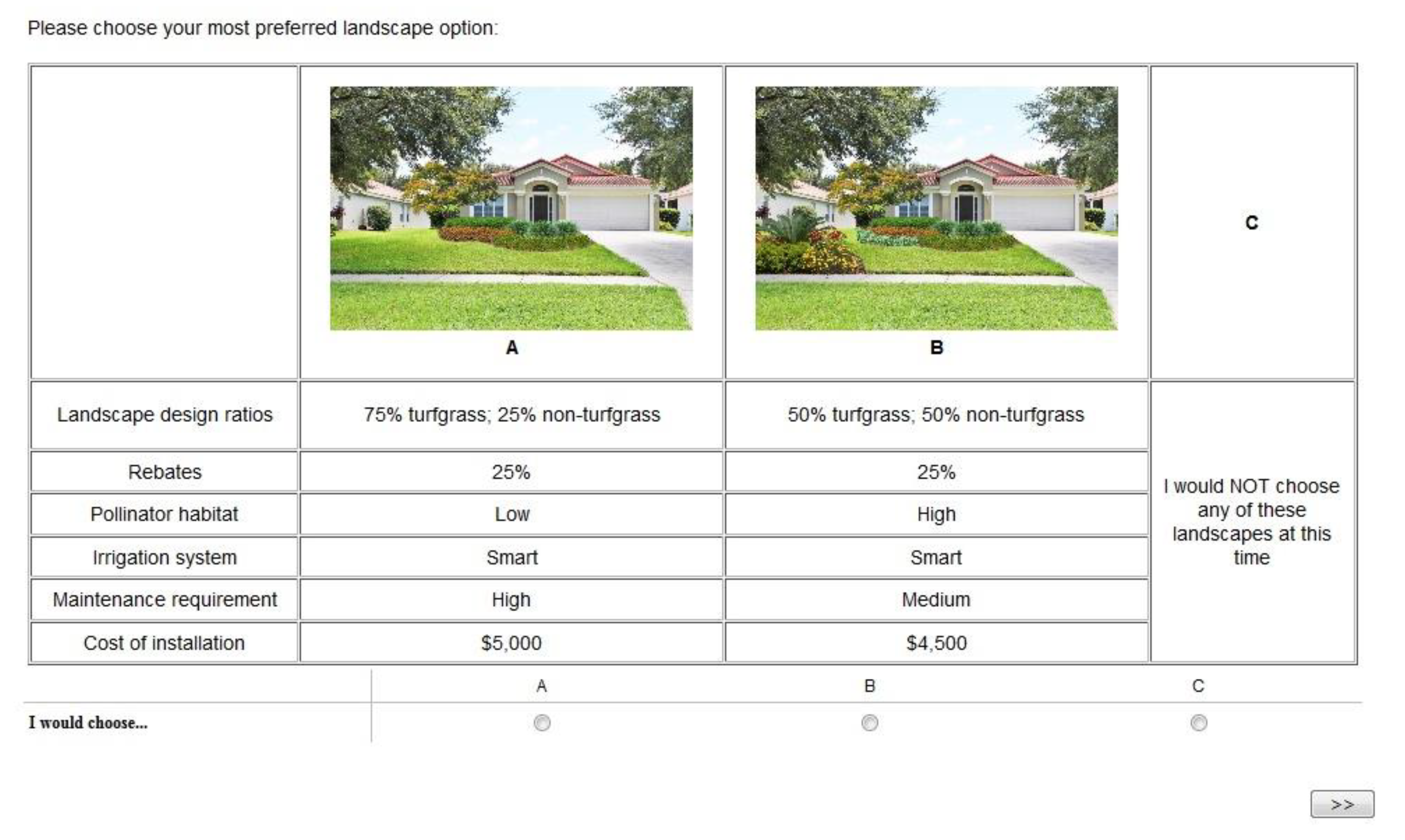
3.1. Design of Choice Experiment

The discrete choice experiment (DCE) method was used to investigate the link between households’ rebate requirement and WTP for specific low-input landscape attributes. DCE methods follow the random utility theory framework and Lancaster’s theory of utility maximization [24] and have been widely used to reveal consumers’ preferences and willingness to pay for environmental goods and services [25]. In this study, the choice scenarios simulated low-input residential landscape designs, and participants were asked to select one of the alternatives based on the tradeoff among multiple alternatives and attributes. The choice question was described in the instruction with the explanation of each attribute. The alternative low-input landscapes with images and descriptive attributes were presented to the participants (Figure 1), while each choice scenario consisted of three options: A, B, or “would not choose”. The opt-out option was defined as respondents were evaluating their preferences for not choosing over the other two alternatives. The site-specific information was standardized across all choices as follows: lot size was assumed to be 0.25 acres (10,890 sq. ft.); landscape area was 0.11 acres (5000 sq. ft.), and house price was $250,000 (i.e., median house price in Florida [26]).
The landscape attributes were developed by three rounds of focus group discussions among researchers and landscape designers. Six landscape attributes were reflective of a range of socio-ecological concerns raised within the focus group, including low-input landscape design ratio, pollinator-friendly habitat, smart irrigation, maintenance requirement level, cost of installation, and rebate incentive level. The four levels of landscape design ratios show the percentage of turfgrass and plant area in the landscape (Table 1). For example, 75% turfgrass/25% plant (Plant25) represented 75% of turfgrass area and 25% is plant (i.e., shrubs, perennials, annuals, trees, mulch, etc.), which is treated as the traditional design [27]. Alternative landscape design ratios include 50% turfgrass with 50% plant (Plant50), 25% turfgrass with 75% plant (Plant75), and 100% plant (did not include turfgrass) (Plant100).
Low-input landscape attributes also include pollinator-friendly habitat, smart irrigation system, and maintenance requirement level, with respective attribute levels ranging from two to four (Table 1). The cost of installation is included in each option with four levels, which were also estimated based on information provided by professional landscape designers. Three rebate incentive levels are included to simulate rebate incentives.
The choice experiment was designed by the Design of Experiment routine in JMP Pro 11 (JMP®). Considering the cognitive burden and fatigue of asking participants to evaluate a full factorial design of 576 scenarios, we used a fractional-factorial orthogonal design and constructed 16 choice profiles with a D-efficiency of 90.3%. These profiles were blocked into two with eight choice scenarios in each, and respondents were evenly and randomly assigned to one of the two choice blocks.

3.2. Survey Instrument

An online survey was conducted in November of 2016 by survey software platform CoreXM developed by Qualtrics Inc., which maintains a panel of Floridian consumers. After confirming the participation, the choice experiment instruction was presented to participants prior to the experiment to standardize and facilitate the choice process. The purpose of the instructions was to ensure respondents’ understanding about the experiment and ameliorate the hypothetical bias of the DCE. Participants were screened based on the following criteria: (1) lived in a single-family house with a certain type of irrigated landscape, and (2) maintained their lawn/garden or landscapes themselves. In addition, half of the participants were randomly assigned to receive environmental benefits information as the treatment group.
After completing the choice experiment, a question asked participants’ monetary incentive requirement threshold: “How much of a rebate would you need in order to consider installing an alternative landscape?” Respondents used the slide-the-scale between 0–100 percent to select their preferred rebate rate. Respondents’ incentive requirement thresholds were then categorized into three segments, i.e., low, medium, and high incentive requirement level. The cut-off values correspond to less or equal to 25 percent, between 25 percent and 50 percent, and greater than 50 percent, respectively. The criteria were selected according to the rebate incentive levels that are commonly applied by landscape conservation programs [17]. Respondents’ socio-demographic information was collected in the last part of the survey.

3.3. Econometric Models

Respondents may have heterogeneous preferences for landscape attributes. To account for heterogeneous preference structure, the mixed logit model (ML) was employed. The mixed logit model allows the attribute parameters to vary and relaxes the assumption of independence of irrelevant alternatives (IIA) [28]. The utility function can be described as:
Unjt = Xnjt βn + εnjt
where individual n (n = 1, …, N) chooses alternative j with the preferred attributes among J alternatives in t choice set. Xnjt is a vector of observed attribute variables, including landscape design ratio, rebate incentive, pollinator-friendly habitat, smart irrigation, maintenance requirement, and installation cost. βn indicates the random parameter vector that is unknown and varies with the density function φ(β|θ), where θ is the true parameters of distribution for attributes preferences. εnjt is assumed to be independent and identically distributed with type I extreme value (Gumbel) distribution.
In the mixed logit model, the choice probability that individual n would choose alternative i in choice scenario t can be expressed as:
P r n i t ( y n = i ) = e x p ( β X n i t ) j = 1 J exp ( β X n j t ) ϕ ( β | θ ) d β , for   i = 1 , , J
Since β is unknown, the unconditional probability is employed based on the distribution of β. As φ(.) is the density function of a multivariate normal distribution, we can estimate the θ parameters, which are the mean and variances for the multivariate normal distribution.
To derive the economic implications, WTP estimates were calculated by using the negative ratio of non-price attribute coefficient to price attribute coefficient. Investigating WTP for underlying attributes is a widely used practice for assessing consumers’ preference for environmentally friendly goods [29]. In addition, the coefficient for installation cost variable is also assumed random. As with other coefficients with normal distribution, the estimation of WTP in preference space often results in undefined distribution [30,31]. Either the WTP distribution is unknown from dividing two normal distributed coefficients, or the value of the denominator is close to zero and the WTP estimates become extremely large [32,33]. Hence, we applied the mixed logit model in WTP space following Hole and Kolstad [30] and Train and Weeks [31].
Equation (3) is the model in preference space.
U n j t = ( α n / k n ) c o s t n j t + ( β n / k n ) x n j t + ε n j t ,   j   =   1 , ,   J ,   t   =   1 ,   ,   T
where costnjt is the installation cost of alternative j in scenario t for individual n, α is the price coefficient, and ε n j t is independent and identically distributed as Type I Extreme Value (Gumbel), with constant variance π 2 / 6 . The scale parameter kn captures variance over observations in factors not observed. The coefficients are defined as λ n = ( α n / k n ) and c n = ( β n / k n ) , such that Equation (3) can be rewritten as:
U n j t = λ n c o s t n j t + c n x n j t + ε n j t
In the WTP space model, WTP is directly estimated as opposed to the derivation using the negative ratio of the attribute and price coefficients in the preference space, w n = c n / λ n [30]. Then, the latent utility function in the WTP space is:
U n j t = λ n [ c o s t n j t + w n x n j t ] + ε n j t
since the cost coefficient is assumed to have a log-normally distributed coefficient and the WTP coefficients are to be normally distributed. The variable costnjt is converted to negative value (as −cost) in the regression so that not only can λn be non-negative and log-normal distributed, but also the WTP for attributes, wn, can be directly estimated (without changing signs). Similar to the mixed logit (ML) model in preference space, the estimation of the mixed logit model in WTP space also uses a maximizing simulated likelihood L L ( θ ) =   n = 1 N ln Pr n ( θ ) . Because there is no closed form for the log likelihood function, this expression cannot be solved analytically: it is approximated using simulation methods, and the ML produces a set of means and standard deviations of the parameters [28]. The estimation was conducted using Stata 13, with 500 Halton draws to simulate the random parameters.

4. Results

4.1. Sample Summary

The online survey was distributed within the state of Florida in November 2016. A total of 610 responses were evenly split into the environmental benefits information treatment group and the control group. The sample summary of socio-demographics is shown in Table 2.
The sample summary shows that fifty-nine percent of respondents are female. The average age is 49.2 years old, slightly older than the census data. Regarding the ethnic distribution, 81.6% of respondents are Caucasian, 7.5% are African American, 5.6% are Hispanic, and 5.4% indicated others. The mean education level is some college to a college degree. About 88.0% of respondents had completed college or above education. In addition, 62.7% are employed (full employment, part-time employment, and self-employed). Annual income levels range from below $19,999 to above $300,000, but most respondents (36.9%) are in the $20,000–$59,999 income range (Table 2). The sample slightly differs from the Florida census data, which might be a result of the qualification screening for survey participation.
Using the incentive requirement threshold for adopting low-input landscapes, respondents can be categorized into three groups. Three incentive requirement thresholds are used for segmenting respondents, i.e., low (required rebate rate ≤ 25%), medium (required rebate rate > 25% and ≤ 50%), and high (required rebate rate > 50%) levels. The sample requirement level is ranged from 0 to 100 percent, and the median level is 45.5%, indicating that households’ incentive requirement levels are comparatively high. The distribution is comparatively even, with 250 respondents in the medium incentive requirement group, 212 respondents in the high incentive requirement group, and the rest in the low incentive requirement group. Although consumers’ average age was slightly different (indicating that older people tended to have relatively low incentive preference), there were no significant demographic differences among the three segments.

4.2. Willingness-to-Pay for Landscape Attributes and Rebate Incentive

WTP estimates were directly obtained from the mixed logit in WTP space model. To assess the differences between consumers with different incentive requirement levels, the WTP estimates were estimated and summarized respectively for the overall sample and for the three groups (with different incentive requirement levels), as well as with and without environmental benefits information treatment, respectively (Table 3).
The results of WTP estimates for the control group of the overall sample provide an overview regarding households’ preferences for landscape features without receiving environmental benefits information (Table 3, column 1). For example, the WTP for 50% turfgrass with 50% plant (Plant50) is $694, and for 100% plant design (Plant100) is −$1510, indicating that households are willing to pay a premium for the low-input landscape designs with up to 50% turfgrass, but do not prefer the designs with 100% plant. The results are in line with a previous study predicting native plant landscaping preference, in which the results indicated that the design ratio of 50% plant and 50% turfgrass was acceptable, but not 100% plant design [34]. Our results also reveal that households prefer low-input landscape attributes. For example, WTP results were significant and positive for the attributes such as pollinator-friendly habitat ($729), smart irrigation ($401), and low and medium levels of maintenance requirement ($1982 and $1198).
After segmenting respondents into groups by incentive requirement threshold, the results of WTP estimates show substantial differences with different significance levels. For example, landscape design ratios (Plant50 and Plant75) become mostly insignificant, indicating highly heterogeneous preferences, but all respondents certainly disliked the 100% plant design (−$2512 and −$2162 for low and medium incentive preference group respectively).
Respondents with a low incentive requirement threshold show comparatively large WTP for most of the other landscape attributes. For example, the WTP estimates for pollinator-friendly habitat and smart irrigation are statistically significant ($1818 and $666), compared to the results for the respondents in the medium and high incentive requirement groups. In addition, we find that respondents with a high incentive requirement level tend to have higher WTP for the attributes that have economic rather than environmental implications, e.g., maintenance requirement. For example, for the low maintenance requirement level, the WTP estimate ($1926) is greater than that of the other two groups. For the medium maintenance requirement, the WTP is the second highest ($1314), similar to the respondents with a low incentive requirement level ($1346).
The results of the WTP for landscape attributes support part of the first hypothesis (H1a and H1b) that households with low incentive requirement level will be more likely to be willing to pay premiums for low-input landscape design attributes, and households with high monetary incentive requirement level will be less willing to pay premiums for low-input landscape attributes but tend to prefer the attributes that have economic rather than environmental implications.
Respondents’ willingness to participate in a rebate incentive program is also examined. The positive WTP values for two rebate incentive levels indicate that households are willing to install a low-input landscape if rebate incentives are offered. Both rebate levels (25% and 50%) can be effective, e.g., for the overall control group, the WTP estimates for the two rebate levels (Rebate25 and Rebate50) are $598 and $959, with the higher rebate rate (Rebate50) revealed larger marginal utility. For households in different incentive requirement groups, from low to high, the willingness to participate shows a decreasing effect, suggesting respondents with a high incentive requirement threshold may value the same level of incentive much less than those with low incentive requirement level. For example, respondents in the low incentive requirement level group are more willing to participate in the program ($929 for Rebate25 and $1253 for Rebate50), compared with respondents in the high incentive requirement level group ($716 for Rebate25 and $999 for Rebate50). Although rebate incentive can be effective in general as a behavioral nudge, for households with a low incentive requirement level, the effectiveness is comparatively strong.
In sum, the results support the first hypothesis. Households in the low incentive requirement level group are more willing to participate in rebate incentive programs and prefer low-input landscape design attributes, compared to households with higher incentive requirement threshold. In contrast, the rebate incentives tend to be less effective for households with high incentive requirement level on conversion to low-input landscape; households with high incentive requirement level focus on economic-related attributes, but not on low-input landscape design attributes.

4.3. Environmental Benefits Information and Synergistic Effects

The second objective of the study is to test whether environmental benefits information has synergistic effects on landscape preferences. The WTP estimates of the treatment group are shown in columns 6–9 of Table 3, and the last four columns of Table 3 show the WTP differences between the control and treatment group. An equality test was first conducted between the overall control group and the overall treatment group, using the method introduced by Swait and Louviere [35] to test whether the environmental benefits information has an overall effect on WTP estimates. The test result rejected the equality hypothesis (χ221 = 64.628, p value = 0.000), indicating the significant effects of the information treatment. In addition, unpaired t-tests are used to assess the equality of WTP estimates between the control group and the information treatment group for each attribute (level). The t-test statistics also indicate significant differences between the compared WTP estimates.
For the overall sample, the environmental benefits information has significant but limited effects. For example, whether respondents received information or not, there are no significant differences for WTP for Plant75 and Plant100, and respondents slightly reduced their WTP for Plant50 (-$312). In terms of other landscape attributes, the environmental benefits information shows effects on respondents’ preference for pollinator attractive habitat, smart irrigation system, and maintenance requirement. Respondents indicate higher WTP (e.g., for pollinator-friendly habitat, $1114 vs. $729, for smart irrigation, $951 vs. $401, and for medium maintenance requirement $1295 vs. $1198). Respondents are also willing to reduce WTP for the low maintenance requirement level slightly (−$141) after receiving the information, suggesting they understand the tradeoff between maintenance requirement and turfgrass lawn designs. Moreover, respondents in the treatment group show an increased WTP ($816 vs. $598) for participating in the rebate 25% program and a lowered WTP ($885 vs. $959) for participating in the rebate 50% program. Respondents tend to be willing to accept low-level rebate programs after receiving the environmental benefits information.
The effects for respondents in different incentive requirement groups are substantially different across the three groups with different incentive requirement levels. For example, the environmental benefits information can have significant effects on respondents with low incentive requirement level but have limited impacts on respondents with medium incentive requirement level. Furthermore, the information treatment shows almost no effects on respondents with high incentive requirement level. Specifically, the WTP estimates have improved for Plant50 for the low incentive requirement group ($822) and for Plant100 for the medium incentive requirement group ($1136), but not for respondents in the high incentive requirement group, compared to the control group. The environmental benefits information also has impacts on other landscape attributes, e.g., maintenance requirement, smart irrigation, and pollinator-friendly habitat. For example, respondents with low incentive requirement level are willing to pay the highest premium for the pollinator-friendly habitat ($1594). For the smart irrigation attribute, the WTP estimates improve significantly for the low and medium incentive requirement groups. For the maintenance requirement attribute, all three groups have improved WTP estimates by receiving the information, and respondents with low incentive requirements significantly improve more ($1158 for Mainlow and $308 for Mainmed).
The synergistic effects between monetary incentive requirement and environmental benefits information exist and indicate various patterns for respondents with different incentive requirement levels. Respondents in the low incentive requirement segment have substantial improvement on Rebate25 ($322) and a big decrease on Rebate50 (−$625), suggesting they are willing to accept a lower level of rebate incentives when the information is provided. In contrast, the information has much less impact on respondents with a high incentive requirement level (the improvement is only $86 for Rebate25 and -$31 for Rebate50). Respondents in the low incentive requirement group indicate the highest WTP for Rebate25 ($1251), and respondents in the high incentive requirement level reflect the highest WTP for Rebate50 ($968). The information treatment further wide spreads the effects of rebate incentives between the two groups.
In sum, the second hypothesis that a synergistic effect exists between monetary incentive requirement and environmental benefits information is supported. Making information about the environmental benefits of maintained landscapes accessible to households can improve their preferences and WTP for selected landscape attributes (H2a). Households’ incentive requirement level can largely influence the significance and magnitude of the effects, and the environmental benefits information has substantial effects on households with low incentive requirement level, but limited effects on households with medium and high incentive requirement level (H2b).

5. Discussion and Conclusions

Most traditional residential landscapes in the United States are designed with proportionally larger turfgrass areas and with relatively small areas devoted to non-turfgrass plant species [36]. Although following the year 2000, total water usage declined slightly for the state of Florida, on average, the per capita daily water consumption is between one hundred and one hundred fifty gallons per day, and water usage should still be a growing concern to Floridians [37].
One of the major hurdles in successful implementation of sustainable urban landscape management programs is to convince households to replace their traditional landscapes with low-input alternatives. Understanding the potential barriers to turfgrass transformation decisions can aid policymakers to implement landscape conservation programs more effectively through a combination of monetary and non-monetary interventions. To provide practical insights for effective implementation of relevant statewide programmatic efforts, the present study investigates the effect of monetary incentives requirement on households’ preferences and willingness to pay for low-input landscape attributes.
While rebate incentives have positive effects on households’ installation intentions, synergistic effects exist when applying the environmental benefits information. This confirms the potential efficacy of combining an educational component with monetary incentives in landscape conservation programming. The effects of information are substantially more significant in households with low incentive requirement levels compared to those with high incentive requirement levels. More specifically, households with low incentive requirement levels are more likely willing to participate in rebate incentive programs and are willing to pay more for low-input landscape attributes, compared to households with medium and high incentive requirement levels. In contrast, limited effects are observed for households with high incentive requirement levels, implying that a high rebate incentive program might not be as effective as expected and that providing rebate incentives to those households may not guarantee significant effects on incentive program participation.
To incentivize households to install low-input landscapes and adopt environmentally friendly landscape practices, existing rebate incentive programs tend to apply high-level rebate incentives (e.g., up to 50%) without tailoring information to target appropriate household segments. These practices could be part of the reason for current low low-input conversion rates, since households’ incentive requirement level may significantly influence the efficacy of rebate incentive programs.
Decision-makers may take into consideration that even when combining educational information into intervention programs, rebate incentives might still not be effective for those households with high incentive requirement levels. Being aware of households’ heterogeneous preferences, our results for households in different incentive requirement groups may insightfully inform about anticipated landscaping practice adoption intentions. Taking households’ incentive requirement into consideration and combining environmental benefits information may be an approach to improve the results of lawn conversion. Particularly, targeting households with low incentive requirement levels may substantially improve the outcome. In addition, policymakers, landscape conservation program developers, and landscape professionals should promote different landscape features for homeowners using tailor-made strategies. Using low-rate rebate incentive as a behavioral nudge for households with low incentive requirement level is preferable. Convincing environmental benefits information should be used for households to improve their environmental perceptions and attitudes before implementing any monetary incentive programs. Hopefully, our findings can be used to refine social marketing programs aimed at changing landscape management practices.
This study is not free of limitations. First, enlarging the sample size might reveal more significant preference estimates after segmenting consumers according to their incentive requirement levels. Second, the sample’s sociodemographic characteristics somewhat echo the earlier findings [38,39] and the National Gardening Association’s study [40] and are slightly skewed towards female respondents, and Caucasians with higher-than-average income. Hence, the interpretation of the findings needs to take this into consideration. Third, future studies can integrate consumers’ psychographic factors, e.g., pro-environmental attitude and perception, to assess their WTP for low-input landscape preferences. The effects of the consumers’ psychographics on the conversion decision of low-input landscapes should be addressed to help develop FFL landscape codes and informed policy decisions.

Author Contributions

H.K. developed the conceptual framework, designed the survey instrument, conducted the survey, and assisted with data analysis and manuscript writing. X.Z. contributed to the development of the conceptual framework, analyzed the data, and wrote the manuscript. All authors have read and agreed to the published version of the manuscript.

Funding

This research was supported by the Center for Landscape Conservation and Ecology at the University of Florida.

Conflicts of Interest

The authors declare no conflict of interest.

References

  1. Environmental Protection Agency (EPA). WaterSense, an EPA Partnership Program. 2016. Available online: https://www3.epa.gov/watersense.html (accessed on 14 March 2017).
  2. Lee, M.; Tansel, B.; Balbin, M. Urban Sustainability Incentives for Residential Water Conservation: Adoption of Multiple High Efficiency Appliances. Water Resour. Manag. 2013, 27, 2531–2540. [Google Scholar] [CrossRef]
  3. Millock, K.; Nauges, C. Household Adoption of Water-Efficient Equipment: The Role of Socio-Economic Factors, Environmental Attitudes and Policy. Environ. Resour. Econ. 2010, 46, 539–565. [Google Scholar] [CrossRef] [Green Version]
  4. Wong, T.H.F.; Brown, R.R. The Water Sensitive City: Principles for Practice. Water Sci. Technol. 2009, 60, 673–682. [Google Scholar] [CrossRef] [Green Version]
  5. Allen, C. A Quantitative Analysis of the Effect of Cash-4-Grass Programs on Water Consumption. In ProQuest Dissertations and Theses; 208; ProQuest: Ann Arbor, MI, USA, 2014. [Google Scholar]
  6. Environmental Protection Agency (EPA). Reduce Your Outdoor Water Use. 2013. Available online: https://www.epa.gov/sites/production/files/2017-03/documents/ws-factsheet-outdoor-water-use-in-the-us.pdf (accessed on 14 March 2017).
  7. Katzev, R.D.; Johnson, T.R. Comparing the Effects of Monetary Incentives and Foot-in-the-Door Strategies in Promoting Residential Electricity Conservation. J. Appl. Soc. Psychol. 1984, 14, 12–27. [Google Scholar] [CrossRef]
  8. Winett, R.A.; Kaiser, S.; Haberkorn, G. The Effects of Monetary Rebates and Daily Feedback on Electricity Conservation. J. Environ. Syst. 1976, 6, 329–341. [Google Scholar] [CrossRef]
  9. Winkler, R.C.; Winett, R.A. Behavioral Interventions in Resource Conservation: A Systems Approach Based on Behavioral Economics. Am. Psychol. 1982, 37, 421–435. [Google Scholar] [CrossRef]
  10. Bennear, L.S.; Taylor, L.; Lee, J. Participation Incentives, Rebound Effects and the Cost-Effectiveness of Rebates for Water-Efficient Appliances. SSRN Electron. J. 2011. [Google Scholar] [CrossRef]
  11. Campbell, H.E.; Johnson, R.M.; Larson, E.H. Prices, Devices, People, or Rules: The Relative Effectiveness of Policy Instruments in Water Conservation1. Rev. Policy Res. 2004, 21, 637–662. [Google Scholar] [CrossRef]
  12. Energy Star. Energy Star Overview. 2016. Available online: https://www.energystar.gov/about (accessed on 14 March 2017).
  13. Gilg, A.; Barr, S. Behavioural Attitudes towards Water Saving? Evidence from a Study of Environmental Actions. Ecol. Econ. 2006, 57, 400–414. [Google Scholar] [CrossRef]
  14. Clem, T.B. Extension Landscape Programs and the Values-Beliefs-Norms Theory: Studying the Impacts of Extension Programs and Beer Anticipating Environmental Behavior Change. Ph.D. Thesis, University of Florida, Gainesville, FL, USA, 2017. [Google Scholar]
  15. Metropolitan Water District of Southern California. SoCal Water$mart|Residential Rebates, Sacramento, CA. 2017. Available online: http://socalwatersmart.com/?page_id=3007 (accessed on 14 March 2017).
  16. Southern Nevada Water Authority. Water Smart Landscapes Rebate. 2016. Available online: https://www.snwa.com/rebates/wsl/index.html (accessed on 14 March 2017).
  17. Alachua County Environmental Protection Department. Turf SWAP Program. Gainesville, FL. 2017. Available online: http://www.alachuacounty.us/Depts/epd/WaterResources/myyardourwater/TurfSWAP/Pages/default.aspx (accessed on 14 May 2017).
  18. Stern, P.C. Information, Incentives, and Proenvironmental Consumer Behavior. J. Consum. Policy 1999, 22, 461–478. [Google Scholar] [CrossRef]
  19. Environmental Protection Agency (EPA). Customer Incentives for Water Conservation. 1994. Available online: https://nepis.epa.gov/Exe/ZyNET.exe/40000KLY.TXT?ZyActionD=ZyDocument&Client=EPA&Index=1991+Thru+1994&Docs=&Query=&Time=&EndTime=&SearchMethod=1&TocRestrict=n&Toc=&TocEntry=&QField=&QFieldYear=&QFieldMonth=&QFieldDay=&IntQFieldOp=0&ExtQFieldOp=0&XmlQuery=&File=D%3A%5Czyfiles%5CIndex%20Data%5C91thru94%5CTxt%5C00000014%5C40000KLY.txt&User=ANONYMOUS&Password=anonymous&SortMethod=h%7C-&MaximumDocuments=1&FuzzyDegree=0&ImageQuality=r75g8/r75g8/x150y150g16/i425&Display=hpfr&DefSeekPage=x&SearchBack=ZyActionL&Back=ZyActionS&BackDesc=Results%20page&MaximumPages=1&ZyEntry=1&SeekPage=x&ZyPURL (accessed on 14 March 2017).
  20. Hanak, E.; Davis, M. California Economic Policy: Lawns and Water Demand in California; Public Policy Institute of California: San Francisco, CA, USA, 2006. [Google Scholar]
  21. Harlan, S.L.; Yabiku, S.T.; Larsen, L.; Brazel, A.J. Household Water Consumption in an Arid City: Affluence, Affordance, and Attitudes. Soc. Nat. Resour. 2009, 22, 691–709. [Google Scholar] [CrossRef]
  22. Addink, S. Cash for Grass—A Cost Effective Method to Conserve Landscape Water. University of California at Riverside Turfgrass Research Facility. 2008. Available online: http://ucrturf.ucr,edu/topics/Cash-for-Grass.pdf (accessed on 14 May 2017).
  23. Hilaire, R.S.; Hall, S.; Cruces, L.; Arnold, M.A.; Wilkerson, D.C.; Devitt, D.A.; Hurd, B.H.; Lesikar, B.J.; Lohr, V.I.; Martin, C.A.; et al. Efficient Water Use in Residential Urban Landscapes. HortScience 2008, 43, 2081–2092. [Google Scholar] [CrossRef]
  24. Lancaster, K.J. A New Approach to Consumer Theory. J. Polit. Econ. 1996, 74, 132–157. [Google Scholar] [CrossRef]
  25. Johnston, R.J.; Boyle, K.J.; Adamowicz, W.; Bennett, J.; Brouwer, R.; Cameron, T.A.; Hanemann, W.M.; Hanley, N.; Ryan, M.; Scarpa, R.; et al. Contemporary guidance for stated preference studies. J. Assoc. Environ. Resour. Econ. 2017, 4, 319–405. [Google Scholar] [CrossRef] [Green Version]
  26. U.S. Census Bureau. Quick Facts. 2017. Available online: https://www.census.gov/quickfacts/fact/table/FL,US/PST045217 (accessed on 14 March 2017).
  27. University of Florida Institute of Food and Agricultural Sciences (UF/IFAS). The Florida Yards and Neighborhoods Handbook. 2015. Available online: https://ffl.ifas.ufl.edu/materials/FYN_Handbook_2015_web.pdf (accessed on 14 May 2017).
  28. Train, K.E. Discrete Choice Methods with Simulation; Cambridge University Press: Cambridge, UK, 2009. [Google Scholar]
  29. Khachatryan, H.; Suh, D.H.; Zhou, G.; Dukes, M. Sustainable Urban Landscaping: Consumer Preferences and Willingness to Pay for Turfgrass Fertilizers. Can. J. Agric. Econ. 2017, 65, 385–407. [Google Scholar] [CrossRef]
  30. Hole, A.R.; Kolstad, J.R. Mixed Logit Estimation of Willingness to Pay Distributions: A Comparison of Models in Preference and WTP Space Using Data from a Health-Related Choice Experiment. Empir. Econ. 2012, 42, 445–469. [Google Scholar] [CrossRef]
  31. Train, K.E.; Weeks, M. Discrete Choice Models in Preference Space and Willingness-to-Pay Space. Appl. Simul. Methods Environ. Resour. Econ. 2005, 3, 1–16. [Google Scholar] [CrossRef] [Green Version]
  32. Scarpa, R.; Thiene, M.; Train, K. Utility in Willingness to Pay Space: A Tool to Address Confounding Random Scale Effects in Destination Choice to the Alps. Am. J. Agric. Econ. 2008, 90, 994–1010. [Google Scholar] [CrossRef]
  33. Xie, J.; Gao, Z.; Swisher, M.; Zhao, X. Consumers’ Preferences for Fresh Broccolis: Interactive Effects between Country of Origin and Organic Labels. Agric. Econ. 2016, 47, 181–191. [Google Scholar] [CrossRef]
  34. Peterson, M.N.; Thurmond, B.; Mchale, M.; Rodriguez, S.; Bondell, H.D.; Cook, M. Predicting Native Plant Landscaping Preferences in Urban Areas. Sustain. Cities Soc. 2012, 5, 70–76. [Google Scholar] [CrossRef]
  35. Swait, J.; Louviere, J.J. The Role of the Scale Parameter in the Estimation and Comparison of Multinomial Logit Models. J. Mark. Res. 1993, 30, 305. [Google Scholar] [CrossRef]
  36. Robbins, P.; Birkenholtz, T. Turfgrass Revolution: Measuring the Expansion of the American Lawn. Land Use Policy 2003, 20, 181–194. [Google Scholar] [CrossRef]
  37. U.S. Geological Survey (USGS). Historical Water-Use in Florida. United States Geological Survey. 15 September 2016. Available online: http://fl.water.usgs.gov/infodata/wateruse/historical.html (accessed on 14 May 2017).
  38. Khachatryan, H.; Suh, D.H.; Xu, W.; Useche, P.; Dukes, M. Towards Sustainable Water Management: Consumer Preferences and Willingness to Pay for Smart Irrigation Technologies. Land Use Policy 2019, 85, 33–41. [Google Scholar] [CrossRef]
  39. Suh, D.H.; Khachatryan, H.; Rihn, A.; Dukes, M. Relating Knowledge and Perceptions of Sustainable Water Management to Preferences for Smart Irrigation Technology. Sustainability 2017, 9, 607. [Google Scholar] [CrossRef] [Green Version]
  40. National Gardening Association. The National Gardening Association’s Comprehensive Study of Consumer Gardening Practices, Trends, and Product Sales; National Gardening Association Inc.: Williston, VT, USA, 2013. [Google Scholar]
Figure 1. Choice scenario example.
Water 12 03023 g001
Table 1. Alternative low-input landscape attributes and attribute levels.
AttributesLevelsVariable
Cost of installation ($)$4500, $5000, $5500, $6000Cost
Landscape design ratio75% turfgrass/25% plant (base)
50% turfgrass/50% plant
25% turfgrass/75% plant
100% plant
Plant25
Plant50
Plant75
Plant100
Rebate levels
 
 
Pollinator attractive habitat
 
0% (base)
25%
50%
High
Low (base)
Rebate0
Rebate25
Rebate50
Habitat
Irrigation systemSmart
Conventional (base)
Irrigation
Maintenance requirementLow
Medium
High (base)
Maintlow
Maintmed
Mainthigh
Table 2. Summary statistics of socio-demographics characteristics.
Whole SampleControl GroupTreatment GroupU.S. Census Group b
Observations610305305-
Age49.249.349.041.1 a
Female (%)59.060.357.751.1
Ethnic Group (%)
Caucasian81.682.680.754.9
African American7.56.68.216.8
Hispanic5.65.95.324.9
Others5.44.94.63.4
Education (%)
High school12.010.113.830.0
College degree (2 years above)68.570.266.945.0
Graduate degree19.519.719.38.0
Employment (%)
Employed full time46.646.946.253.6
Employed part time8.27.98.5-
Self-employed7.96.98.8-
Unemployed7.98.96.94.9
Student1.21.01.3-
Retired25.725.925.619.7
Income (%)
Less than $19,9993.84.92.618.8
$20,000–$59,99936.937.136.739.4
$60,000–$99,99933.330.136.422.3
$100,000 above26.127.924.219.6
a Florida’s mean age includes individuals under 18 years old whereas the sample does not include minors. b Data from the U.S. Census Bureau [26].
Table 3. Homeowners’ willingness to pay for environmentally friendly landscapes attributes, by monetary incentive preference.
Control GroupTreatment GroupWTP Difference (Treatment-Control)
AttributesOverall
Control
Group
N = 305
(1)
Low Incentive Requirement
N = 80
(2)
Medium Incentive Requirement
N = 128
(3)
High Incentive Requirement
N = 97
(4)
Overall Treatment Group
N = 305
(5)
Low Incentive Requirement
N = 68
(6)
Medium Incentive Requirement
N = 122
(7)
High Incentive Requirement
N = 115
(8)
ΔWTP (Overall)ΔWTP
(Low Incentive Requirement)
ΔWTP
(Medium Incentive Requirement)
ΔWTP
(High Incentive Requirement)
Mean Estimates
Plant500.694 ***0.5470.627 *0.4990.382 *1.3690.0880.357−0.312 ***0.822 ***−0.539***−0.142
(0.252)(0.465)(0.343)(0.329)(0.200)(0.974)(0.223)(0.317)[0.01][0.008][0.001][0.395]
Plant750.103−0.1260.1220.2300.2340.8780.0980.1420.1311.004−0.024−0.088
(0.246)(0.583)(0.310)(0.366)(0.225)(0.797)(0.241)(0.354)[0.23][0.200][0.870][0.766]
Plant100−1.510 ***−2.512 ***−2.162 **−0.311−1.588 ***−1.313−1.026 **−2.274 **−0.0781.1991.136 **−1.963 ***
(0.560)(0.898)(0.921)(0.692)(0.540)(2.119)(0.448)(0.947)[0.43][0.362][0.039][0.008]
Habitat0.729 ***1.818 ***0.745 **0.916 **1.114 ***1.594 **1.127 ***0.771 **0.385 ***−0.224 **0.382 ***−0.145
(0.209)(0.569)(0.300)(0.365)(0.226)(0.726)(0.272)(0.346)[0.00][0.010][0.001][0.374]
Irrigation0.401 **0.666**0.3990.625 **0.951 ***1.331 **0.975 ***0.557 **0.550 ***1.996 **0.576 ***−0.068
(0.169)(0.323)(0.262)(0.295)(0.189)(0.642)(0.234)(0.274)[0.00][0.022][0.000][0.471]
Mainlow1.982 ***1.504 **1.913 ***1.926 ***1.841 ***2.662 *1.377 ***1.799 ***−0.141 *1.158 ***−0.536 ***−0.127 *
(0.456)(0.767)(0.669)(0.697)(0.422)(1.610)(0.431)(0.684)[0.05][0.000][0.002][0.054]
Mainmed1.198 ***1.346 **0.953 **1.314 ***1.295 ***1.6541.003 ***1.256 **0.097 ***0.308 ***0.050 ***−0.058
(0.304)(0.582)(0.391)(0.484)(0.307)(1.023)(0.313)(0.500)[0.00][0.000][0.000][0.387]
Rebate250.598 ***0.929 **0.752 ***0.716 **0.816 ***1.251 *0.638 ***0.802 **0.218 ***0.322 ***−0.114 ***0.086 **
(0.171)(0.407) (0.284)(0.295)(0.190)(0.697)(0.203)(0.313)[0.00][0.001][0.003][0.040]
Rebate500.959 ***1.253 **1.075 ***0.999 ***0.885 ***0.6280.676 ***0.968 **−0.074 **−0.625 ***−0.399 ***−0.031
(0.254)(0.600)(0.400)(0.368)(0.238)(0.791)(0.258)(0.408)[0.04][0.000][0.000][0.560]
Scale(λ)−0.560 ***−0.611−0.667 **−0.608 **−0.574 ***−0.708−0.407**−0.649 **
(0.180)(0.377)(0.260)(0.288)(0.171)(0.465)(0.198)(0.276)
Optout−8.224 ***−12.58 ***−8.22 ***−5.49 ***−7.334 ***−7.595 ***−6.196 ***−7.923 ***
(0.853)(0.377)(1.135)(0.736)(0.682)(1.607)(0.609)(1.088)
Standard Deviation
Plant501.637 ***2.132 ***1.309 ***1.145 **1.447 ***1.251 *0.638 ***0.802 **
(0.363)(0.693)(0.475)(0.449)(0.351)(0.697)(0.203)(0.313)
Plant752.213 ***2.675 ***1.301 *2.162 ***2.082 ***4.334 *1.007 ***2.122 ***
(0.470)(1.013)(0.666)(0.774)(0.456)(2.286)(0.351)(0.737)
Plant1006.293 ***5.703 ***5.572 ***4.526 ***5.313 ***9.9732.382 ***5.829 ***
(1.379)(1.725)(1.799)(1.430)(1.169)(6.371)(0.892)(1.998)
Habitat1.175 ***0.4750.8090.6761.097 ***0.5670.960 **1.479 ***
(0.312)(0.343)(0.631)(0.435)(0.319)(0.608)(0.406)(0.535)
Irrigation0.6291.083 **0.4710.846 **0.5722.296 *0.4940.506
(0.445)(0.463)(0.454)(0.396)(0.377)(1.338)(0.346)(0.551)
Mainlow1.275 ***0.746 *1.544 **0.693 *0.8441.7191.141 *0.106
(0.456)(0.404)(0.769)(0.380)(0.552)(1.087)(0.621)(1.021)
Mainmed0.1040.1990.1930.2080.0340.0950.1240.630
(0.193)(0.257)(0.306)(0.283)(0.237)(0.443)(0.334)(0.404)
Scale(λ)0.579 ***1.316 ***0.0470.666***0.499 ***0.4130.1970.227
(0.200)(0.457)(0.176)(0.185)(0.154)(0.312)(0.178)(0.156)
Optout5.727 ***9.558 ***5.007 ***7.044 ***4.416 ***6.002 **3.428 ***3.474 ***
(1.160)(3.339)(1.423)(2.076)(0.826)(2.789)(0.771)(1.071)
# of Obs.73201920307223287320163229282760
Log-likeli-hood−2018.827−511.538−849.856−652.946−2032.899−417.212−829.783−765.423
Note: Baseline attributes are shown in the first column. Simulations were conducted using 500 Halton draws. Willingness to pay (WTP) values are in $1000 dollars. The cost coefficient was assumed to have a log-normally distributed coefficient. *, **, *** represent significance at the 10%, 5%, and 1% levels, respectively. Standard errors for WTP estimates are in parentheses. WTP differences (ΔWTP) tested by unpaired t-test. p values in square brackets are reported in the last four columns.
Publisher’s Note: MDPI stays neutral with regard to jurisdictional claims in published maps and institutional affiliations.

