Article

A Novel Approach to Harmonize Vulnerability Assessment in Carbonate and Detrital Aquifers at Basin Scale

by
Leticia Baena-Ruiz
* and
David Pulido-Velazquez
Spanish Geological Survey (IGME), Urb. Alcázar del Genil, 4. Edificio Zulema, bajo, 18006 Granada, Spain
*
Author to whom correspondence should be addressed.
Water 2020, 12(11), 2971; https://doi.org/10.3390/w12112971
Submission received: 23 September 2020 / Revised: 19 October 2020 / Accepted: 21 October 2020 / Published: 23 October 2020
(This article belongs to the Special Issue Assessing Water Quality by Statistical Methods)

Abstract

:
The DRASTIC (D: Depth to water; R: Net recharge; A: Aquifer media; S: Soil media; T: Topography; I: Impact of vadose zone; C: Hydraulic conductivity) index is usually applied to assess intrinsic vulnerability in detrital and carbonate aquifers, although it does not take into account the particularities of karst systems as the COP (C: Concentration of flow; O: Overlying layers above water table; P: precipitation) method does. In this paper we aim to find a reasonable correspondence between the vulnerability maps obtained using these two methods. We adapt the DRASTIC index in order to obtain reliable assessments in carbonate aquifers while maintaining its original conceptual formulation. This approach is analogous to the hypothesis of “equivalent porous medium”, which applies to karstic aquifers the numerical solution developed for detrital aquifers. We applied our novel method to the Upper Guadiana Basin, which contains both carbonate and detrital aquifers. Validation analysis demonstrated a higher confidence in the vulnerability assessment provided by the COP method in the carbonate aquifers. The proposed method solves an optimization problem to minimize the differences between the assessments provided by the modified DRASTIC and COP methods. Decision trees and spatial statistics analyses were combined to identify the ranges and weights of DRASTIC parameters to produce an optimal solution that matches the COP vulnerability classification for carbonate aquifers in 75% of the area, while maintaining a reliable assessment of the detrital aquifers in the Basin.

Graphical Abstract

1. Introduction

Groundwater pollution is a widespread problem affecting most aquifers all over the world due to the increasing agricultural and industrial human activity [1,2]. It is the result of the interaction between the anthroposphere and the hydrosphere, where substances from the different land uses penetrate the groundwater, leading to impacts on environmental water quality and human health. The protection of the groundwater resources has become a priority due to the importance of groundwater for human supply, irrigation and dependent ecosystems, especially in semi-arid regions [3,4,5]. The degree of protection depends on intrinsic groundwater vulnerability, which is defined as the susceptibility of aquifers to pollution arising from anthropogenic activity [6]. Several methods have been proposed to assess intrinsic vulnerability by using conceptual groundwater flow models and taking transport processes into account [7,8]. The most frequently employed methods are the index-based approaches [9,10] of which DRASTIC (D: Depth to water; R: Net recharge; A: Aquifer media; S: Soil media; T: Topography; I: Impact of vadose zone; C: Hydraulic conductivity) [9] is the most common. DRASTIC has been applied to various types of aquifer, though some authors have revealed that it is not suitable for assessing vulnerability in some karstic aquifers [10,11,12,13].
Karstic aquifers present physical particularities that, in general, make them more sensitive to contamination [14,15]. Specific approaches, such as the COP (C: Concentration of flow; O: Overlying layers above water table; P: precipitation) method [10], have been developed specifically to assess groundwater vulnerability in carbonate (karstic) aquifers. The COP method has been extensively applied in different research studies to this type of aquifer [16,17,18,19,20,21].
However, despite significant physical differences between detrital and karstic aquifers, the same approaches are often applied to simulate groundwater processes in both types of aquifers. In numerical groundwater flow models, the “equivalent porous medium” assumes the validity of the Darcy’s law in karstic aquifers, which is the most frequent numerical approach deduced for detrital aquifers. We find many examples of application of this approach both for detrital aquifers [22,23,24] and karstic aquifers [25,26]. In the same way, index methods such as DRASTIC could be suited to assessing vulnerability in both detrital and karstic aquifers.
In this context, recent research studies have attempted to adapt the DRASTIC method to karst aquifers in recent years [12,27,28,29,30]. Some of these [12,28,29] modified DRASTIC by including and/or removing parameters to account for karst characteristics. Other studies [27,30] adapted DRASTIC by modifying the classic assessment according to the distribution of nitrate concentration, although the most contaminated areas do not always imply higher vulnerability [31,32]. A detailed review of different approaches proposed to modify the DRASTIC method is given in [13].
These modifications of the DRASTIC method were performed using different methodologies/approaches: single-parameter sensitivity analysis [3,5,33], calibration by correlation analysis with pollutants [4,34,35], analytic hierarchy process [36,37,38] amongst others. Different data mining algorithms have also been applied to improve DRASTIC performance [39,40,41,42], predict areas vulnerable to groundwater contamination or to identify hydrogeological factors influencing groundwater contamination [39,43,44]. Data mining algorithms aim to extract knowledge from previously unknown and indistinguishable data, and are used as operational tools to find optimal solutions in high-dimension problems. Although many authors have employed these techniques for different purposes, more research is needed to explore the potential of the statistical techniques—including data mining—to deal with the uncertainties in the weights and ratings of index-based methods in the groundwater vulnerability assessments [45].
In general, the aforementioned index-based methods have been proven to provide satisfactory vulnerability assessment in a variety of regions. However, different index methods often provide dissimilar results in a single study area, making it difficult to compare and validate results [46,47,48]. In complex groundwater systems containing various aquifers types, an integrated vulnerability assessment is needed to homogenize criteria and compare results at basin scale and between different case studies. In general, a harmonized method that is applicable to all aquifer types would be more likely to be implemented worldwide [12,49]. Previous work [12] has aimed at developing a new method (DRISTPI; Depth to water, Recharge, Impact of vadose zone, Soil, Topography, Preferential Infiltration) by adding and removing certain parameters from the classic DRASTIC method that can be applied to any type of aquifer. It was tested in karstic aquifers, but not in detrital aquifers.
In this paper we propose a novel approach to standardize the DRASTIC method to assess vulnerability in a basin composed by both, detrital and carbonate aquifers. We proposed an adaptation of the most commonly applied method for detrital aquifers—the DRASTIC method—to obtain a reliable vulnerability assessment for carbonate aquifers. The DRASTIC method can be applied in both detrital and carbonate aquifers, though it does not always provide appropriate vulnerability assessment in carbonate aquifers. In contrast, the COP method is specific to carbonate aquifers and it yielded better results in the validation analysis in our case study. Therefore, we proposed to adapt DRASTIC to harmonize the vulnerability assessment for different aquifer typologies, in order to make the results comparable in a basin that contains a wide variety of geological formations. Harmonization of criteria in the vulnerability assessment would allow the dissimilarities provided by different vulnerability methods to be dealt with. Although in the literature we can find several attempts to adapt the DRASTIC method to the particularities of each case study, none of them have proved the applicability of the modified DRASTIC in different aquifer typologies.
In this study, an optimization problem is solved to establish a correspondence between DRASTIC and COP by maintaining the original formulation of the DRASTIC method. It aims to find the weights and ranges of the DRASTIC parameters that maximize the correspondence between the qualitative vulnerability classes obtained using DRASTIC and COP methods. The optimization problem is solved through a new approach that combines spatial statistics analysis and data mining (decision trees). Although decision trees have been applied to predict the sensitivity to contaminants based on groundwater vulnerability [50,51], they have not been used to adapt/improve the DRASTIC method.
The optimization methodology was applied to five carbonate aquifers in the Upper Guadiana Basin, where the validation analysis demonstrated that COP method produces better vulnerability assessment than the original DRASTIC one. The optimal solution obtained for carbonate aquifers (O-DRASTIC) was also tested in the three detrital aquifers within the basin and the validation analysis also shows significant improvement in the results comparing with the original DRASTIC. A sensitivity analysis of the changes introduced to define the optimum DRASTIC reveals the influence of the various intrinsic characteristics on the severity of vulnerability for different aquifer typologies.

2. Materials and Methods

2.1. Study Area and Data

The Upper Guadiana Basin (Figure 1) is located in the central part of Spain. It is composed of eight groundwater bodies including five unconfined mixed (carbonate and detrital) and three unconfined detrital aquifers extending over approximately 14,000 km2.
The climate in this area is typically continental and semiarid. Mean annual precipitation over the period 1974–2015 was 445 mm and the mean annual temperature is 14.7 °C. Mean potential evapotranspiration is 700 mm/year.
The area is predominantly flat, bounded by mountain landscapes to the north (Sierra de Altomira) and south (Campo de Montiel).
Connectivity between groundwater bodies is structurally complex, with strong natural interaction between groundwater and surface water. Under natural conditions groundwater flow discharges into the central aquifer of the system (Mancha Occidental Aquifer) [52] which flows eastwards.
The predominantly dry climate and the prevalence of irrigated agriculture means that the Upper Guadiana Basin has been intensively pumped, and this has led to some of its aquifers being declared overexploited [53]. The water table is highly variable, lying at less than 1 m to more than 250 m, though over most of the basin it lies below 15 m.
Rainfall is the main source of aquifers’ recharge. Mean annual recharge varies between 45 and 70 mm/year, although there is disagreement about these values [52,53,54].
The soils in the basin mainly belong to the cambisol group according to the FAO (Food and Agriculture Organization of the United Nations) classification [54,55]. Regosol and others, such as luvisol and podzol, can be found in the southeast [54]. Soil texture in the northern part of the basin is predominantly silty-loam, whereas the soil in the southern part it is peaty.
The geology is complex, including mixed carbonate–detrital aquifers. In the southern half of the Upper Guadiana Basin, the aquifers are predominantly composed of limestones, with many karstified zones [53]. In general, the karst is not very developed and there are no swallow holes in these aquifers. Many parts of the central aquifer are formed by Tertiary detrital deposits [53]. The northern aquifers are more heterogeneous. There are no large karstified areas and other formations of metamorphic materials can be found. The detrital aquifers are mainly composed of Tertiary and Quaternary alluvial materials.
The unsaturated zone is formed by poorly permeable lithologies in the northern part of the basin, with higher permeabilities in the southern part [54].
Conductivity in the Upper Guadiana Basin varies widely. To the north, conductivity is low (below 1.5 × 10⁻⁴ m/s); in the central part there are zones with values higher than 5 × 10⁻⁴ m/s, while conductivity to the southern is mainly in the range 3.5 × 10⁻⁴–5 × 10⁻⁴ m/s [56].

2.2. DRASTIC and COP Vulnerability Maps

DRASTIC and COP vulnerability maps were calculated in the five mixed aquifers following the proposal made in [9,10], respectively (Figure 2). A detailed explanation of these methods can be found in the Appendix A. Table A4 and Table A5 (Appendix B) summarizes the data sources and the methodology applied to calculate the parameters of DRASTIC (hereinafter, we will call it “original DRASTIC”) and COP, respectively.
The “original DRASTIC” values vary between 41 and 171 within the study area. The final index was reclassified into five qualitative classes (Very low: <100; Low: 100–120; Moderate: 120–160; High: 160–180; Very high: ≥180) by grouping the original categories proposed in [9] to obtain the same number of classes as the COP vulnerability map. The values of parameters Aquifer media, Soil media, Impact of vadose zone and Conductivity (Figure 2(a3,a4,a6,a7)) show significant heterogeneity, with clear differences between the northern and central–southern areas. These differences are finally reflected in the vulnerability map (Figure 2(a8)).
Figure 2b shows the results of applying the COP method as proposed by [10]. The protection conferred by Overlaying the layers (Figure 2(b2)) generally decreases from north to south. It is very low in the southern part due to the presence of limestones and dolomites outcrops. The surface features related to the Concentration of flow (Figure 3(b1)) produce only a slight reduction of protection over 80% of the area, except in the southern Campo de Montiel aquifer, where the protection from Overlying layers is greatly reduced.
While the highest values of the DRASTIC index are located in the center and southern part of the basin (classified as “Moderate vulnerability”), the highest values of the COP index appear in the southern zone (Campo de Montiel aquifer). Both indices give their lowest values in the north area (Sierra de Altomira and Lillo Quintanar aquifers).
The percentage overlap between the vulnerability classes obtained using COP and DRASTIC is 55.75%. There is a significant coincidence in the “Very low” and “Low” vulnerability classes, which cover nearly 80% of the area in the COP map. However, the coincidence in “High” and “Very high” classes is almost null. A misclassification of the highest vulnerability areas of groundwater dependent ecosystems such as the Upper Guadiana Basin would lead to erroneous planning and management decisions, possibly leading to significant environmental impacts.

2.3. Validation of Vulnerability Maps

Contaminant loads are linked to human activities and land use (LU). Therefore, in addition to aquifer vulnerability, these are a key factor in determining groundwater contamination [3,57]. In the study area, the intensive agriculture and the use of nitrogen fertilizers has provoked high levels of nitrates in many groundwater areas. Since nitrate is not naturally found in groundwater, it is considered to be a good indicator of contamination by human impact, especially in agricultural zones. The DRASTIC vulnerability map is validated by adding an LU factor to the DRASTIC index (Equation (1)), as proposed in other studies [27,58,59]. Making an analogy, the index defining protection against pollution could be based on the COP vulnerability (Equation (2)). In this case the inverse of the LU factor is considered since a higher COP index indicates lower vulnerability levels. Since the principal land use is agriculture, the pollution index and the protection-against-pollution index will maintain the factor of 5 used to weight the LU term, as was originally included in the DRASTIC pollution index by other authors [27,60]:
Pollution   index   ( DRASTIC ) = DRASTIC   index + 5 × LU
Protection against Pollution   index   ( COP ) = COP   index + 5 LU
The rates assigned to LU [3,27,33,34] are shown in Table 1.
The correlations (R-squared coefficient) with the pollution index derived from DRASTIC and COP methods (Figure 3) were determined from the 214 observation points where nitrate concentration data was available (1974 to 2015 provided by the Spanish Geological Survey and the River Basin Authority). The DRASTIC pollution index (Figure 3a) is weakly correlated with the mean nitrate concentration (R2 = 0.04) in the carbonate aquifers. However, the protection-against-pollution index linked to the COP map (Figure 3b) shows strong correlation (R2 = 0.78). Accordingly, in this validation analysis, the COP vulnerability assessment for the study area provides a more reliable assessment than the DRASTIC index one.
As can be observed in Figure 2 and Figure 3, both DRASTIC and COP indices suggest low vulnerability in some zones with high nitrate concentration (in the western part of the basin) that results from the intensive agricultural exploitation since early 1970’s. Thus, groundwater contamination not only depends on intrinsic vulnerability, but also the land use, type of crops, type of irrigation, etc. For this reason, the most contaminated areas do not always correspond to the most vulnerable ones [31,32].

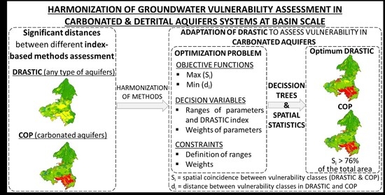
2.4. Methodology: Optimization of DRASTIC Method

In this paper we adapt the DRASTIC method to minimize differences with the COP vulnerability map for the five carbonate aquifers in the Upper Guadiana Basin, which has been proven to provide better results in those aquifers according to the validation analysis. The main objective is to obtain a harmonized method that allows vulnerability in carbonate and detrital aquifers to be assessed in a homogenous way, in a system comprising varying geological formations. The harmonization of criteria to assess groundwater vulnerability will make the results comparable at basin scale. To this end, the DRASTIC index is recalculated by varying the ranges and weights of its parameters (fulfilling certain constraints to maintain a rational definition), in order to minimize the differences with the COP vulnerability map for the five mixed (carbonate and detrital) aquifers in the Upper Guadiana Basin. Data mining techniques are then applied to identify the ranges and weights that provide an optimal solution.
Figure 4 shows the flowchart of the proposed optimization problem and the methodology applied. Two objective functions (O.F.) were tested: (A) to maximize the percentage of spatial coincidence (area, Si) between DRASTIC and COP vulnerability classes; and (B) to minimize the distance (di; see Equation (3)) between the vulnerability classes in DRASTIC and COP. The decision variables in this optimization problem are (1) the ranges (of the DRASTIC index and its parameters) and (2) the weights of the DRASTIC parameters.
The ranges of the DRASTIC parameters and index are proposed based on the available data in the study area and covering a wide range of hypothetical cases. The following constraints regarding the ranges proposal are imposed:
  • The ranges of non-continuous parameters (A, S and I) were assumed to be invariant and we classify these parameters as proposed in [9]. We modify the DRASTIC index classification (DR) and the ranges of only three numerical parameters in DRASTIC: Depth to water (D), Topography (T) and Conductivity (C). The proposed ranges are shown in Table 2. Due to the narrow variability of the data in the study area the recharge ranges were not modified.
  • The number of classes and rates adopted for all parameters are as proposed in [9]. We change only the distribution of numerical data within the ranges in order to adapt them to the characteristics of the case study.
  • The modification of ranges is based on statistical criteria according to the distribution of data in the study area (quantile method, equal intervals, natural clusters in ArcGis and increasing the limit of the ranges by a constant value) [32,61].
  • We established a minimum range amplitude of 5 for the DRASTIC vulnerability classes.
    We also established certain constraints in the weights of parameters:
  • Only weights between 1 to 5 are considered;
  • The sum of the weights had to be 23 for each combination (as the original proposal in [9]).
For each combination of parameter ranges and weights used to generate a DRASTIC map, the distance (di) or difference between vulnerability classes reported by DRASTIC and COP is calculated by Equation (3):
d i = α j k ×   x j k
where
  • αjk is the total area of “j” vulnerability class of COP overlapping with the “k” vulnerability class of DRASTIC;
  • xjk is a weight from 0 to 4 depending on the number of jumps from one vulnerability class to another.
In order to establish a dimensionless threshold to quantify the distance (di), it is expressed as a percentage of the maximum calculated distance (dmax) over all calculated DRASTIC indices:
d i ( % ) = d i d m a x × 100  
In order to reduce the number of calculations, we employ data mining techniques (decision trees) to select the values of the variables domain to be tested. The optimal solution is sought following two steps:
  • Ranges optimization:
    • First, DRASTIC vulnerability maps are calculated modifying the ranges of parameters and the classification of the DRASTIC index. The weights of parameters are the same as proposed in [9].
    • All the DRASTIC indices are evaluated through the objective functions and the results are classified intro three categories (Table 3).
    • Decision trees are applied in order to find out the ranges for each parameter that gives the highest coincidence (Max(Si)) and a lowest distance (Min(di)) between vulnerability classes assigned using DRASTIC and COP.
  • Weights optimization:
    • In this second step, the weights of parameters are introduced as new variables to compute all the feasible combinations of weights and parameter ranges selected in the previous step. The DRASTIC index is calculated for all the combinations of weights and selected classifications in step 1.
    • The new set of DRASTIC maps are evaluated by means of the objective functions.
    • For each parameter, decision trees are applied again to determine the weight that yields greatest similarity between the DRASTIC and COP maps.
The main objective of decision trees in this study is to identify the ranges and weights for each DRASTIC parameter involved in any combination that yields the maximum spatial coincidence (Si) and the minimum distance between vulnerability classes (di) (Si = 3 or di = 1 according to Table 3). We establish these threshold values according to the distribution of results in the first set of combinations. Decision trees reduce the computational cost of the optimization problem and allow the most relevant variables to be identified in the vulnerability assessment in carbonate aquifers.
The CHAID (Chi-square Automatic Interaction Detection) algorithm [62,63] is applied in decision trees, considering the objective functions of the optimization problem (Si and di) as dependent variables. The proposed ranges and weights of parameters and classifications of DRASTIC are the independent variables, and the chi-squared test of significance is used as the splitting criterion in the CHAID algorithm. Each dataset generated in steps 1 and 2 is partitioned into a training set (70%) and a testing set (the remaining 30%) in order to assess the performance of the models. The goodness-of-fit of the classification is evaluated using the precision index [51,64]:
P r e c i s i o n =   n = 1 n = 3 T P n n = 1 n = 3 ( T P n + F P n )
where:
  • n = number of classes;
  • TPn = number of correctly recognized class examples in the class n;
  • FPn = number of examples incorrectly assigned to the class n;
Decision trees can represent the relationship between variables and output class using specific rules following the pathway from the root node to the terminal node [63,65,66]. A priori, the number of terminal nodes on the tree can determine the number of rules but it may generate a large number of irrelevant pieces of information. Only the most relevant variables (rules with the highest population for each decision tree with precision above 50%) whose terminal nodes in the tree are classified as Si = 3 or di = 1 are selected to generate all the feasible combinations to compute the DRASTIC indices.

3. Results

3.1. Optimization of the DRASTIC Method

3.1.1. Ranges Optimization

In the first optimization step, we obtained a total of 11,520 different DRASTIC maps. The spatial coincidence (Si) of the vulnerability classes between the DRASTIC and COP maps rose to 61.31% (from 55.75% in “original DRASTIC”) and the minimum distance between vulnerability classes (di) fell to 20.85% (doriginal DRASTIC = 24.72%).
The selected ranges (from Table 2) for each parameter extracted from decision trees were as follows:
  • DR11, DR12, DR14, DR15 and DR16 for DRASTIC classification;
  • D*, D1, D2, D3 and D4 for Depth to water;
  • T* and T1 for Topography;
  • C7 and C8 for Conductivity.
The ranges proposed in [9] were selected for parameters D and T in the decision tress. For conductivity, the selected classifications (C7 and C8) assign lower rates to conductivity values.

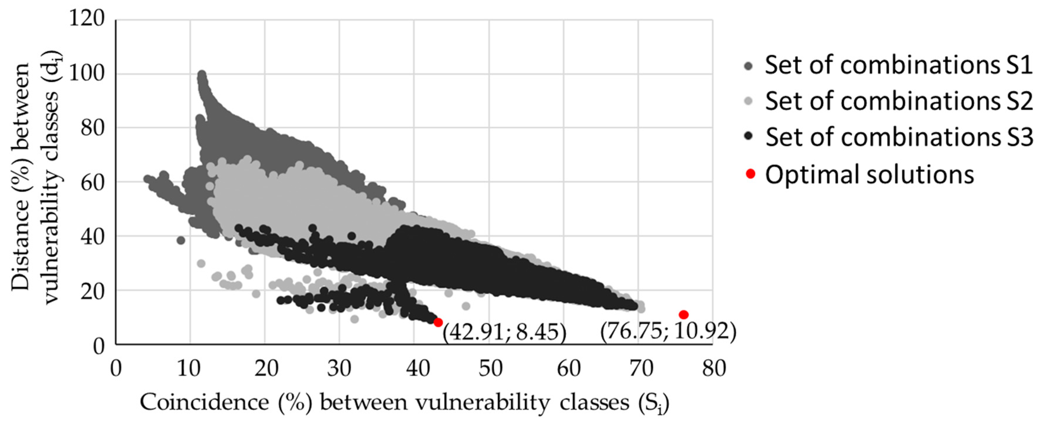
3.1.2. Weights Optimization

The selected ranges for parameters and the DRASTIC index were combined, varying the weights of parameters between one and five. Due to a large number of generated combinations, we first considered weights one, three and five. This resulted in 35,700 new DRASTIC maps. The spatial coincidence (Si) between vulnerability classes increased to 70.34% and the minimum distance between vulnerability classes (di) fell to 8.45%.
Decision trees were applied again to determine the optimum weight for each parameter. We aimed to determine if the value of the weight for each parameter provides relevant information in the optimization problem. We found that a weight equal to five did not appear in relevant rules in parameters D and T, whereas a weight equal to one did not appear for parameters R and S. All weights (one, three, and five) were found in rules for parameters A, I and C.
A new set of combinations of ranges and weights were computed to find an optimum between the gaps left due to constraints. We introduced the mid-weights for each parameter, discarding those not found in the relevant rules. We included the following weights for each parameter: WD = 2; WR = 4; WA = 2 and 4; WS = 4; WT = 2; WI = 2 and 4; WC = 2 and 4. The total of combinations provide two optimal solutions:
  • Optimum of O.F. Min(di): di = 8.45; Si = 42.91;
  • Optimum of O.F. Max(Si): di = 13.05; Si = 70.34;
The second solution was considered the best solution because the gain in Si was higher than the loss in di. Finally, the best solution was refined by adjusting the classification of the DRASTIC index to increase the spatial coincidence with the COP map, obtaining the optimum DRASTIC. The classification of the optimum DRASTIC does not match with the ranges proposed originally in [9]. The objective functions take the following values for the optimum DRASTIC: Si = 76.75%; di = 10.92%.
Figure 5 shows the dot-plot of the all the DRASTIC indices calculated. It reveals the efficacy of using decision trees in the methodology to reduce the number of combinations to be tested when seeking the optimal solution. Each set of combinations improves the objective functions. Black dots show those including the mid-weights for each parameter that produce improvement in the objective function “di”, but not in “Si”. Red dots indicate the DRASTIC indices that provide Max(Si) and Min(di).

3.2. Analysis of Optimum DRASTIC (O-DRASTIC)

O-DRASTIC keeps the ranges proposed in [9] for parameters D and T. Only ranges of parameter C change in O-DRASTIC (C8 from Table 2). In general, the value of the conductivity rates is reduced in O-DRASTIC. The spatial distribution of conductivity ranges shows slight changes. The weights (W) of parameters of O-DRASTIC are shown in Table 4, compared with the original DRASTIC weights.
Results of O-DRASTIC reveal that Depth to water and Conductivity have no a significant impact on vulnerability for our case study area. The ranges of parameter C in O-DRASTIC also support this conclusion given that the new classification of this parameter reduces the rate assigned to conductivity values. This conclusion is confirmed by the single-parameter sensitivity analysis of O-DRASTIC, in which the parameter C takes a mean effective weight of 1.7% (compared to its empirical weight 4.3%). In general, in the study area, the carbonate aquifers have a scarcely developed karst. In fact, approximately half the study area shows lower rates in the conductivity map. Although conductivity takes high values in some zones, the ranges of this parameter change in O-DRASTIC with respect to the original DRASTIC. The new classification in O-DRASTIC assigns lower rates to the conductivity values. Therefore, this parameter losses influence, which is also reflected in the weight. Moreover, conductivity can be considered as implicit in the aquifer media parameter (A), which increased in weight in O-DRASTIC in our case study. The reduced weight of parameter D may be due to the large depth to water table over most of the study area. The mean effective weight obtained in the sensitivity analysis was 3.2% (empirical weight = 4.3%) Aquifer media and Soil media gained great significance in the vulnerability assessment, as well as Recharge, albeit by a reduced amount. Impact of vadose zone continues to be an important factor in O-DRASTIC.
The weights in O-DRASTIC are consistent with the concept of COP methodology, where the vulnerability assessment is based mainly on the degree of protection afforded by overlying layers and the way in which the water percolates (recharges) into the aquifer.
The main changes between the original and optimum DRASTIC vulnerability maps mostly occur in areas of “Very low” and “Moderate” vulnerability of the original DRASTIC, since these are the predominant classes in this vulnerability map. Remarkably, those changes do not always occur in one direction. “Moderate” vulnerability shifts towards “Low” or “Very high” vulnerability depending on the zone, whereas other “Moderate” vulnerability areas remain with the same class. In the same way, some “Very low” vulnerability zones jump up a vulnerability class to “Low”, while other maintain the same class. We analyzed the differences in the distribution of the parameter rates in these areas.
Figure 6a shows that the main factor causing the vulnerability to change from “Moderate” to “Low” is Depth to water. Since the weight of this parameter changed from five to one in O-DRASTIC, zones with higher rates of D report a greater fall in the vulnerability value, leading the vulnerability class to drop by one level. This graph also shows how some areas with rates of three, five and seven change from “Moderate” to “High” vulnerability, which demonstrates that other parameters influence the “Very high” vulnerability class.
On the other hand, we can observe in Figure 6a that the rate of parameter S (soil media) is equal to eight over more than 80% of the area where vulnerability increased from “Moderate” to “Very high”, corresponding with soils with a high organic content, and outcrops of limestone and dolomites. Furthermore, the rate of S is equal to four over nearly 90% of the area where vulnerability fell from “Moderate” to “Low”. Zones where no change in vulnerability class was observed have soils with medium values.
A similar conclusion regarding Soil media is drawn in the areas where vulnerability rose from “Very low” to “Low” (Figure 6b). In these zones we can also observe higher rates of parameters A (aquifer media) and I (impact of vadose zone). These zones correspond to karstified areas and highly permeable layers.
The results highlight the influence of Aquifer media, Soil media and Impact of vadose zone in the vulnerability of carbonate aquifers.
These conclusions are supported by the single-parameter sensitivity analysis carried out for O-DRASTIC, which yields higher effective weights in parameters A, S and I and lower effective weights for parameters D and C.
In general, the new ranges of Conductivity in O-DRASTIC contribute to an overall drop in vulnerability class, but the weights of parameters cause a sharp jump in vulnerability class, especially in the southern part of the basin, where Aquifer media and Soil media have the greatest influence (higher rates in this area).
The values of the optimum DRASTIC (O-DRASTIC) vary between 52 and 178 and the optimal vulnerability classes are the following:
  • “Very low”: 52–107;
  • “Low”: 107–130;
  • “Moderate”: 130–138;
  • “High”: 138–146;
  • “Very high”: ≥146;
Figure 7a shows a better distribution of vulnerability values in O-DRASTIC within the COP vulnerability classes (compared to the original DRASTIC). Close similarities can also be appreciated between the O-DRASTIC and COP vulnerability maps (Figure 7b). The vulnerability classes in O-DRASTIC overlap with COP over 76.75% of the basin, representing an improvement of 20% relative to the original DRASTIC. This spatial coincidence is particularly improved in the class of “Very high” vulnerability, with a 90% coincidence between COP and O-DRASTIC.
O-DRASTIC was validated using the pollution index (Equation (1)) and the correlation with nitrate concentration (R2 = 0.653) in carbonate aquifers improved with respect to the original DRASTIC).
Lastly, we assessed the vulnerability of the three detrital aquifers in the Upper Guadiana Basin by applying original DRASTIC and O-DRASTIC, and we validated the maps following Equation (1). Original DRASTIC showed a good correlation (R2 = 0.765) in detrital aquifers but O-DRASTIC gave a significantly better correlation (R2 = 0.862). Both methods (original DRASTIC and O-DRASTIC) perform a better vulnerability assessment in detrital aquifers than in carbonate aquifers.
Figure 8 shows the change that O-DRASTIC produces (compared to original DRASTIC) in terms of distance between vulnerability classes. Negative values mean the vulnerability class drops in O-DRASTIC compared to original DRASTIC, while positive values mean the vulnerability class in O-DRASTIC is higher than in original DRASTIC. Three zones are thus distinguished in the Upper Guadiana Basin: the southern area (Campo de Montiel) where vulnerability increases by one or two classes. This area is characterized by a higher recharge rate and a karstified aquifer. In the mid-basin (including Mancha Occidental I, Mancha Occidental II, Consuegra Villacañas and Rus-Valdelobos), vulnerability decreases generally by one class, although most of the area remains unchanged; in the northern zone (Lillo-Quintanar, Sierra de Altomira and La Obispalía) only small areas jump up a vulnerability class, and by only one level.
The largest difference in vulnerability class assigned is for carbonate aquifers. More than 17% of the carbonate aquifers area rises by two classes or more vulnerability classes. Only 7% of the detrital aquifers area jumps by this much, while 62% of the detrital aquifers show no change in the vulnerability class.

4. Discussion and Conclusions

This paper demonstrates that the DRASTIC method can be adapted to assess vulnerability in carbonate aquifers by undertaking some simple modifications of the weights and ranges of the parameters. Most recent studies to adapt the DRASTIC method to carbonate aquifers have aimed to transform DRASTIC by including and/or removing parameters that take the karst characteristics into account [12,28,29]. Other studies modified the classic assessment according to nitrate concentrations [27,30], though the most highly contaminated groundwater does not always imply higher vulnerability [31,32]. Instead of using either of these previous approaches, our study establishes a correspondence between DRASTIC and a vulnerability method that was specifically developed for karstic aquifers, the COP method, and therefore we avoid making conceptual changes in the original definition of DRASTIC method.
Our methodology is based on an optimization approach that identifies the ranges and weights of DRASTIC parameters that minimize the differences in the vulnerability assessment compared with the COP method, which was developed specifically for karstic aquifers. It allows us to identify the significance of the different DRASTIC parameters in the vulnerability assessment in karstic aquifers. Decision trees and spatial statistics analyses are combined to identify the ranges and weights of parameters that provide the optimal DRASTIC classes in terms of coincidence and distance with the COP vulnerability map. This optimization approach could be applied by minimizing the differences with respect to any other reference method for assessing vulnerability, whose results has been previously validated and considered as reasonable. Although many data mining techniques have been applied in groundwater vulnerability assessments [39,40,42], only a few studies have used decision trees in vulnerability studies [50,51]. They have been mainly used to assess other groundwater quality problems [65,67,68].
Our proposed method was applied in the Upper Guadiana Basin, an agricultural area that overlies carbonate and detrital aquifers. The socio-economic and hydrogeological particularities of the basin highlight the need to establish unified management measures at basin scale, not only regarding groundwater exploitation but also in terms of protecting the good quality of the groundwater resource. Therefore, harmonization of criteria to assess groundwater vulnerability would allow comparison at basin scale and overcome the issue of dissonant results provided by contrasting vulnerability methods. Our approach assumes that the COP method provides a better approximation of the vulnerability in the case study. This assumption was tested by means of a validation analysis in which we show that the “protection-against-pollution” index (derived from COP and LU data) more closely correlates (R2 = 0.78) with nitrate concentration than the DRASTIC “pollution index”. The results of the validation show that the pollution index derived from the original DRASTIC for carbonate aquifers is not correlated with nitrates (R2 = 0.04), whereas in detrital aquifers there is a close correlation ((R2 = 0.76). Other authors have previously pointed out that the original DRASTIC method does not significantly correlate with nitrate concentration in agricultural areas [45,59,69]. In contrast, the pollution index derived from O-DRASTIC shows significant correlation with nitrates for both, carbonate and detrital aquifers (R2 = 0.65 and R2 = 0.86, respectively).
The optimal solution (O-DRASTIC) obtained in this optimization problem shows that changing the range of the Conductivity parameter produces a small drop in the vulnerability class compared with the original DRASTIC but does not lead to a significant improvement in the objective functions (coincidence and distance between vulnerability classes). The reduced significance of Conductivity is also confirmed by the much-reduced weight assigned to this parameter in O-DRASTIC. Other DRASTIC adaptation for carbonate aquifers also pointed the reduced significance of Conductivity to assess the potential “protection-against-pollution” in karstic systems [12]. We also observed a reduced significance of the Depth to water table in our case study (WD = 1). Other research studies that modified the weights of DRASTIC parameters [3,69,70] also found the Depth to water parameter to be insignificant. Specifically in karstic aquifers Depth to water is not so relevant in protecting an aquifer from contamination because of the high transit velocity through the vadose zone [12]. Moreover, the low significance of in our case study may be due to fact that the water table lies below 30 m over most of the basin. The same argument was also stated in another case study [3]. The reduced significance of Depth to water and Conductivity is confirmed by a sensitivity analysis. Topography and Impact of vadose zone maintain their weights (WT and WI) as defined in the original DRASTIC, while the remaining parameters (Recharge, Aquifer media and Soil media) are given maximum weights (WR = WA = WS = 5). The large increments in the weights given to Aquifer media and Soil media in O-DRASTIC show that they are the most significant factors controlling the vulnerability in karstic aquifers. Other authors concur that these parameters are the most significant [3,70,71]. The principal change in O-DRASTIC with respect to the original DRASTIC is in the weights of parameters, which highlights that these parameters embrace most of the uncertainty in the DRASTIC vulnerability assessment [72].
Our optimal solution provides an improvement of 20% in terms of coincidence between the vulnerability classes assigned by DRASTIC and COP. This improvement was achieved by applying spatial statistical analyses and decision trees, which allowed potential solutions to be obtained by exploring only a 0.1% of the total dimensionality of the defined optimization problem. The proposed method also helps to achieve a better understanding of the parameters and variables of the “equivalent detrital approach” that really influence vulnerability in this karstic system. This optimal solution was tested for the carbonate and detrital aquifers in our case study, but it should also be tested in other different aquifers with similar hydrogeological characteristics in order to prove its applicability in a broader context under different management framework.
In summary, results show that COP and O-DRASTIC report higher vulnerability classes than the original DRASTIC method over 36% of the total area overlying carbonate aquifers. The greatest differences between the original DRASTIC and O-DRASTIC are produced for the carbonate aquifers rather than the detrital aquifers. This confirms that the reliability of DRASTIC vulnerability assessment is significantly better for detrital aquifers than for karst aquifers. These underestimations of vulnerability in karstic aquifers when applying the classic DRASTIC is due to the physical particularities of these aquifers and their greater sensitivity to pollution [1,12,31].

Hypotheses, Limitations and Future Works

We have demonstrated the applicability of the method in the case of carbonate aquifers where the karst is not highly developed. Its applicability to well-developed karst aquifers also needs to be tested. The main adopted assumptions and limitations of the general methodology adopted are:
  • The ranges of categorical non-continuous parameters (Aquifer media, Soil media and Impact of vadose zone) are not modified in this optimization procedure. We consider that the Delphi criteria proposed in [9] can be applied to establish the relative significance of each range with respect to potential pollution.
  • Other algorithms and/or techniques (for example, a Random Forest algorithm) could be employed to achieve the goal in a more efficient way.
  • We have not studied the whole domain of potential solutions, and a wider spectrum of parameter ranges could be tested to find other optimal solutions. Moreover, the optimization procedure provides local optimum solutions.
  • Although decision trees help to reduce the dimensionality of the optimization problem, the methodology involves a large number of calculations, which might handicap extending the method to other case studies.
  • The proposed methodology requires a previous validated vulnerability assessment in the study area in order to optimize the DRASTIC method.
Future work should be developed to verify the applicability of O-DRASTIC in other case studies, including aquifers with different physical (climatic and hydrogeological settings) and management particularities in order to withdrawal more generalized conclusions.

Author Contributions

Conceptualization, L.B.-R. and D.P.-V.; Data curation, L.B.-R.; Investigation, L.B.-R.; Methodology, L.B.-R. and D.P.-V.; Software, L.B.-R.; Supervision, D.P.-V.; Validation, L.B.-R.; Visualization, L.B.-R.; Writing—original draft, L.B.-R. and D.P.-V.; Writing—review and editing, L.B.-R. and D.P.-V. All authors have read and agreed to the published version of the manuscript.

Funding

This research did not receive any specific grant from funding agencies in the public, commercial, or not-for-profit sectors.

Acknowledgments

This paper was partially supported by the SIGLO-AN (RTI2018-101397-B-I00) project from the Spanish Ministry of Science, Innovation and Universities (Programa Estatal de I+D+I orientada a los Retos de la Sociedad), the GeoE.171.008-HOVER and the GeoE.171.008-TACTICproject from GeoERA organization funded by European Union’s Horizon 2020 research and innovation program.

Conflicts of Interest

The authors declare that they have no known competing financial interests or personal relationships that could have appeared to influence the work reported in this paper.

Appendix A. DRASTIC and COP Methods

Appendix A.1. DRASTIC Method

DRASTIC method was developed by [9] to assess intrinsic groundwater vulnerability in any type of aquifer.
This method considers that there are seven parameters/variables influencing the vulnerability to contamination: Depth to water table (D), Net recharge (R), Aquifer media (A), Soil media (S), Topography (T), Impact of vadose zone (I) and Hydraulic conductivity (C). A rate of importance is assigned to the parameters according to the value or characteristics of each parameter (Table A1).
Table A1. Ranges and rates for DRASTIC parameters.
Groundwater Table Depth
Original Ranges (ft)Transformed Ranges (m)Original Ratings
0–50–1.510
5–151.5–4.69
15–304.6–9.17
30–509.1–15.25
50–7515.1–22.93
75–10022.9–30.52
>100>30.51
Net Recharge
Original Ranges (inches)Transformed Ranges (mm)Original Ratings
0–20–50.81
2–450.8–101.63
4–7101.6–177.86
7–10177.8–254.08
>10>254.09
Aquifer Media
Original RangesOriginal Ranges
Massive shale2
Metamorphic/Igneous3
Weathered metamorphic/Igneous4
Thin bedded sandstone, Limestone, Shale sequences6
Massive sandstone6
Massive limestone6
Sand and gravel8
Basalt9
Karst limestone10
Soil Media
Original RangesOriginal Ranges
Thin or absent10
Gravel10
Sand9
Peat8
Shrinking and/or aggregated clay7
Sandy loam6
Loam5
Silty loam4
Clay loam3
Muck2
Nonshrinking and nonaggregated clay1
Topography (% Slope)
Original RangesOriginal Ranges
0–210
2–69
6–125
12–183
>181
Impact of Vadose Zone
Original RangesOriginal Ranges
Silt/Clay1
Shale3
Limestone6
Sandstone6
Bedded limestone, sandstone, shale6
Sand and gravel with significant silt and clay6
Metamorphic/Igneous4
Sand and gravel8
Basalt9
Karst limestone10
Hydraulic Conductivity
Original Ranges (GPD/FT2)Transformed Ranges (m/s)Original Ratings
1–1004.7 × 10−7–4.7 × 10−51
100–3004.7 × 10−5–1.4 × 10−42
300–7001.4 × 10−4–3.3 × 10−44
700–10003.3 × 10−4–4.7 × 10−46
1000–20004.7 × 10−4–9.3 × 10−48
>2000>9.3 × 10−410
The values of the parameters are weighted to obtain the DRASTIC index, which is calculated following Equation (A1):
DRASTIC   index = 5 × D + 4 × R + 3 × A + 2 × S + 1 × T + 5 × I + 3 × C
The DRASTIC index was originally classified into eight vulnerability levels according to some color codes [9] (Table A2) although it is usually grouped into five vulnerability classes that do not match with the original proposal in [9].
Table A2. Color codes for the DRASTIC index.
DRASTIC IndexColor Code
<79Violet
80–99Indigo
100–119Blue
120–139Dark Green
140–159Light Green
160–179Yellow
180–199Orange
>200Red

Appendix A.2. COP Method

The COP method was developed by [10] to assess intrinsic groundwater vulnerability in carbonate aquifers.
This method considers the properties of layers overlying the water table (O factor), the concentration of flow (C factor) and precipitation (P factor) as the main parameters influencing groundwater vulnerability in carbonate aquifers. The concept of this method is to assess the natural protection of groundwater determined by the overlying soils and the unsaturated zone, which may be modified by the infiltration process and climatic conditions.
Each factor is divided into subfactors, whose formulation is detailed explained in [10]. The factors are classified in ranges and the COP index calculated as the product of the three factors following the Equation (A2):
COP   index = C × O × P
The ranges of factors and the COP index are shown in Table A3.
Table A3. Values for COP parameters and vulnerability classes for the COP index.
C FactorO Factorp FactorCOP Index
RangesReduction of ProtectionRangesProtection ValueRangesReduction of ProtectionRangesVulnerability Classes
0–0.2Very high1Very low0.4–0.5Very high0–0.5Very high
0.2–0.4High2Low0.6High0.5–1High
0.4–0.6Moderate2–4Moderate0.7Moderate1–2Moderate
0.6–0.8Low4–8High0.8Low2–4Low
0.8–1.0Very low8–15Very high0.9–1Very low4–15Very low

Appendix B. Data Source and Methodology to Calculate DRASTIC and COP

Table A4. Data source and methodology to calculate DRASTIC parameters.
FactorData SourceMethodology
DData from simulation flow model (River Basin Authority) (mean of the simulated data for each grid point from 1974 to 2015).Spatial interpolation using IDW (Inverse Distance Weighted) of groundwater level data and reclassification into D index values.
RRecharge time series calculated from SACRAMENTO model. Mean recharge value in the period 1974–2015.Estimation of the mean net recharge taking into account the different hydrology cycle variables in the period 1974–2015.
AHydrogeological map of Spain 1:200,000.Direct assignment of A index values for each hydrogeological unit delimitated.
SSoil Map of Spain 1:1,000,000.Direct assignment of S index values for each soil type.
TDigital Terrain Model at 100 × 100 m cell size.Calculation of the slope raster file and reclassification of values into T index values.
ILithostratigraphic map of Spain 1:200,000.Direct assignment of I index values for each lithostratigraphic unit.
CFlow model at 1000 × 1000 m cell size.Spatial interpolation using IDW of conductivity data and reclassification into C index values.
Table A5. Data source and methodology to calculate COP parameters.
FactorSubfactorData SourceMethodology
C--There are no catchment areas to swallow holes in these aquifers.
Scenario 2Vegetation from CORINE LAND COVER and slope from Digital Terrain Model (100 × 100 m cell size)
Karstic features from previous research works & fieldwork and litthostratigraphic map 1:200,000.
Carbonate lithologies with low karstification are considered as fissured formations. Limestones and dolomites with high or very high permeability are considered as scarcely developed karst. For sv factor, the vegetation cover is considered high when more than 30% of the surface is covered.
Assignment of the values for the karstic features, vegetation and slope according to COP methodology.
OOS—SoilSoil Map of Spain 1:1,000,000.Assignment of the Os values after classify the different types of soil according to the COP methodology.
OL—LithologyLithostratigraphic map of Spain 1:200,000.Classification of each lithology according to COP methodology and determination of thickness of vadose zone from 3D flow model.
PPQ—Precipitation quantityPrecipitation data from SPAIN02 [73] in the grid within the Upper Guadiana Basin (mean rainfall taking into account data above 0.5 mm/day).Reclassification of the precipitation values into the PQ subfactor values, taking into account the average rainfall in the wet years.
Precipitation series from SPAIN02 between 1974 and 2015 were used to extract the mean annual precipitation for wet years.
PI—Temporal distributionPrecipitation data from SPAIN02 (number of rainy days in the grid within the Upper Guadiana Basin).Counting of the number of rainy days above 0.5 mm for each cell in the SPAIN02 grid.
For the estimate of the rainy days per year, meteorological historical series between 1974 and 2015 from SPAIN02 were analysed.

References

  1. Kazakis, N.; Voudouris, K.S. Groundwater vulnerability and pollution risk assessment of porous aquifers to nitrate: Modifying the DRASTIC method using quantitative parameters. J. Hydrol. 2015, 525, 13–25. [Google Scholar] [CrossRef]
  2. Kadkhodaie, F.; Moghaddam, A.A.; Barzegar, R.; Gharekhani, M.; Kadkhodaie, A. Optimizing the DRASTIC vulnerability approach to overcome the subjectivity: A case study from Shabestar plain, Iran. Arab. J. Geosci. 2019, 12, 527. [Google Scholar] [CrossRef]
  3. Al-Hanbali, A.; Kondoh, A. Groundwater vulnerability assessment and evaluation of human activity impact (HAI) within the Dead Sea groundwater basin, Jordan. Hydrogeol. J. 2008, 16, 499–510. [Google Scholar] [CrossRef]
  4. Javadi, S.; Kavehkar, N.; Mousavizadeh, M.H.; Mohammadi, K. Modification of DRASTIC model to map groundwater vulnerability to pollution using nitrate measurements in agricultural areas. J. Agric. Sci. Technol. 2011, 13, 239–249. [Google Scholar]
  5. Neshat, A.; Pradhan, B.; Dadras, M. Groundwater vulnerability assessment using an improved DRASTIC method in GIS. Resour. Conserv. Recycl. 2014, 86, 74–86. [Google Scholar] [CrossRef]
  6. Foster, S.S.D. Fundamental concepts in aquifer vulnerability, pollution risk and protection strategy. Hydrol. Resour. Proc. Inf. 1987, 38, 69–86. [Google Scholar]
  7. Sonnenborg, T.O.; Scharling, P.B.; Hinsby, K.; Rasmussen, E.S.; Engesgaard, P. Aquifer Vulnerability Assessment Based on Sequence Stratigraphic and 39 Ar Transport Modeling. Ground Water 2015, 54, 214–230. [Google Scholar] [CrossRef]
  8. Seifert, D.; Sonnenborg, T.O.; Scharling, P.; Hinsby, K. Use of alternative conceptual models to assess the impact of a buried valley on groundwater vulnerability. Hydrogeol. J. 2007, 16, 659–674. [Google Scholar] [CrossRef]
  9. Aller, L.; Bennett, T.; Lehr, J.H.; Petty, R.J.; Hackett, G. DRASTIC: A Standardized System for Evaluating Groundwater Potential Using Hydrogeologic Settings; EPA/600/2-85/018; U.S. Environmental Protection Agency: Washington, DC, USA, 1987.
  10. Vías, J.M.; Andreo, B.; Perles, M.J.; Carrasco, F.; Vadillo, I.; Jiménez, P. Proposed method for groundwater vulnerability mapping in carbonate (karstic) aquifers: The COP method. Hydrogeol. J. 2006, 14, 912–925. [Google Scholar] [CrossRef]
  11. Moratalla, A.; Gómez-Alday, J.; Sanz, D.; Castaño, S.; Heras, J.D.L. Evaluation of a GIS-Based Integrated Vulnerability Risk Assessment for the Mancha Oriental System (SE Spain). Water Resour. Manag. 2011, 25, 3677–3697. [Google Scholar] [CrossRef]
  12. Jiménez-Madrid, A.; Carrasco, F.; Martínez, C.; Gogu, R.C. DRISTPI, a new groundwater vulnerability mapping method for use in karstic and non-karstic aquifers. Q. J. Eng. Geol. Hydrogeol. 2013, 46, 245–255. [Google Scholar] [CrossRef]
  13. Barbulescu, A. Assessing Groundwater Vulnerability: DRASTIC and DRASTIC-Like Methods: A Review. Water 2020, 12, 1356. [Google Scholar] [CrossRef]
  14. Vallejos, A.; Andreu, J.M.; Sola, F.; Pulido-Bosch, A. The anthropogenic impact on Mediterranean karst aquifers: Cases of some Spanish aquifers. Environ. Earth Sci. 2015, 74, 185–198. [Google Scholar] [CrossRef]
  15. Goldscheider, N.; Chen, Z.; Auler, A.S.; Bakalowicz, M.; Broda, S.; Drew, D.; Hartmann, J.; Jiang, G.; Moosdorf, N.; Stevanovic, Z.; et al. Global distribution of carbonate rocks and karst water resources. Hydrogeol. J. 2020, 28, 1661–1677. [Google Scholar] [CrossRef] [Green Version]
  16. Ravbar, N.; Goldscheider, N. Comparative application of four methods of groundwater vulnerability mapping in a Slovene karst catchment. Hydrogeol. J. 2008, 17, 725–733. [Google Scholar] [CrossRef] [Green Version]
  17. Plan, L.; Decker, K.; Faber, R.; Wagreich, M.; Grasemann, B. Karst morphology and groundwater vulnerability of high alpine karst plateaus. Environ. Earth Sci. 2008, 58, 285–297. [Google Scholar] [CrossRef]
  18. Polemio, M.; Casarano, D.; Limoni, P.P. Karstic aquifer vulnerability assessment methods and results at a test site (Apulia, southern Italy). Nat. Hazards Earth Syst. Sci. 2009, 9, 1461–1470. [Google Scholar] [CrossRef]
  19. Jiménez-Madrid, A.; Martínez-Navarrete, C.; Carrasco-Cantos, F. Groundwater Risk Intensity Assessment. Application to Carbonate Aquifers of the Western Mediterranean (Southern Spain). Geodin. Acta 2010, 23, 101–111. [Google Scholar] [CrossRef]
  20. Marín, A.I.; Dörfliger, N.; Andreo, B. Comparative application of two methods (COP and PaPRIKa) for groundwater vulnerability mapping in Mediterranean karst aquifers (France and Spain). Environ. Earth Sci. 2011, 65, 2407–2421. [Google Scholar] [CrossRef]
  21. Bagherzadeh, S.; Kalantari, N.; Nobandegani, A.F.; Derakhshan, Z.; Conti, G.O.; Ferrante, M.; Malekahmadi, R. Groundwater vulnerability assessment in karstic aquifers using COP method. Environ. Sci. Pollut. Res. 2018, 25, 18960–18979. [Google Scholar] [CrossRef]
  22. Velázquez, D.P.; Sahuquillo, A.; Andreu, J. A two-step explicit solution of the Boussinesq equation for efficient simulation of unconfined aquifers in conjunctive-use models. Water Resour. Res. 2006, 42, 4205423. [Google Scholar] [CrossRef]
  23. Pulido-Velazquez, D.; Sahuquillo, A.; Andreu, J.; Pulido-Velazquez, M. A general methodology to simulate groundwater flow of unconfined aquifers with a reduced computational cost. J. Hydrol. 2007, 338, 42–56. [Google Scholar] [CrossRef]
  24. Llopis-Albert, C.; Pulido-Velazquez, D. Using MODFLOW code to approach transient hydraulic head with a sharp-interface solution. Hydrol. Process. 2014, 29, 2052–2064. [Google Scholar] [CrossRef]
  25. Pulido-Velazquez, D.; Sahuquillo, A.; Andreu, J.; Pulido-Velazquez, M. An efficient conceptual model to simulate surface water body-aquifer interaction in conjunctive use management models. Water Resour. Res. 2007, 43, 07407. [Google Scholar] [CrossRef]
  26. Velázquez, D.P.; Sahuquillo, A.; Andreu, J. Treatment on non-linear boundary conditions in groundwater modeling with Eigenvalue Methods. J. Hydrol. 2009, 368, 194–204. [Google Scholar] [CrossRef]
  27. Panagopoulos, G.P.; Antonakos, A.K.; Lambrakis, N.J. Optimization of the DRASTIC method for groundwater vulnerability assessment via the use of simple statistical methods and GIS. Hydrogeol. J. 2006, 14, 894–911. [Google Scholar] [CrossRef]
  28. Rózkowski, J. Evaluation of intrinsic vulnerability of an Upper Jurassic karst-fissured aquifer in the Jura Krakowska (southern Poland) to anthropogenic pollution using the DRASTIC method. Geol. Q. 2007, 51, 17–26. [Google Scholar]
  29. Mimi, Z.A.; Mahmoud, N.; Abu Madi, M. Modified DRASTIC assessment for intrinsic vulnerability mapping of karst aquifers: A case study. Environ. Earth Sci. 2011, 66, 447–456. [Google Scholar] [CrossRef]
  30. Pacheco, F.; Pires, L.; Santos, R.; Fernandes, L.S. Factor weighting in DRASTIC modeling. Sci. Total Environ. 2015, 505, 474–486. [Google Scholar] [CrossRef]
  31. Baalousha, H.M. Vulnerability assessment for the Gaza Strip, Palestine using DRASTIC. Environ. Earth Sci. 2006, 50, 405–414. [Google Scholar] [CrossRef]
  32. Hamza, S.M.; Ahsan, A.; Imteaz, M.A.; Rahman, A.; Mohammad, T.A.; Ghazali, A.H. Accomplishment and subjectivity of GIS-based DRASTIC groundwater vulnerability assessment method: A review. Environ. Earth Sci. 2014, 73, 3063–3076. [Google Scholar] [CrossRef]
  33. Saidi, S.; Bouri, S.; Ben Dhia, H. Groundwater vulnerability and risk mapping of the Hajeb-jelma aquifer (Central Tunisia) using a GIS-based DRASTIC model. Environ. Earth Sci. 2009, 59, 1579–1588. [Google Scholar] [CrossRef]
  34. Antonakos, A.; Lambrakis, N. Development and testing of three hybrid methods for the assessment of aquifer vulnerability to nitrates, based on the drastic model, an example from NE Korinthia, Greece. J. Hydrol. 2007, 333, 288–304. [Google Scholar] [CrossRef]
  35. Huan, H.; Wang, J.; Teng, Y. Assessment and validation of groundwater vulnerability to nitrate based on a modified DRASTIC model: A case study in Jilin City of northeast China. Sci. Total Environ. 2012, 440, 14–23. [Google Scholar] [CrossRef] [PubMed]
  36. Thirumalaivasan, D.; Karmegam, M.; Venugopal, K. AHP-DRASTIC: Software for specific aquifer vulnerability assessment using DRASTIC model and GIS. Environ. Model. Softw. 2003, 18, 645–656. [Google Scholar] [CrossRef]
  37. Hailin, Y.; Ligang, X.; Chang, Y.; Jiaxing, X. Evaluation of Groundwater Vulnerability with Improved DRASTIC Method. Procedia Environ. Sci. 2011, 10, 2690–2695. [Google Scholar] [CrossRef] [Green Version]
  38. Sener, E.; Davraz, A. Assessment of groundwater vulnerability based on a modified DRASTIC model, GIS and an analytic hierarchy process (AHP) method: The case of Egirdir Lake basin (Isparta, Turkey). Hydrogeol. J. 2012, 21, 701–714. [Google Scholar] [CrossRef]
  39. Fijani, E.; Nadiri, A.A.; Asghari-Moghaddam, A.; Tsai, F.T.-C.; Dixon, B. Optimization of DRASTIC method by supervised committee machine artificial intelligence to assess groundwater vulnerability for Maragheh–Bonab plain aquifer, Iran. J. Hydrol. 2013, 503, 89–100. [Google Scholar] [CrossRef]
  40. Barzegar, R.; Moghaddam, A.A.; Baghban, H. A supervised committee machine artificial intelligent for improving DRASTIC method to assess groundwater contamination risk: A case study from Tabriz plain aquifer, Iran. Stoch. Environ. Res. Risk Assess. 2015, 30, 883–899. [Google Scholar] [CrossRef]
  41. Jang, W.S.; Engel, B.A.; Harbor, J.; Theller, L. Aquifer Vulnerability Assessment for Sustainable Groundwater Management Using DRASTIC. Water 2017, 9, 792. [Google Scholar] [CrossRef] [Green Version]
  42. Nadiri, A.A.; Gharekhani, M.; Khatibi, R. Mapping Aquifer Vulnerability Indices Using Artificial Intelligence-running Multiple Frameworks (AIMF) with Supervised and Unsupervised Learning. Water Resour. Manag. 2018, 32, 3023–3040. [Google Scholar] [CrossRef]
  43. Dixon, B. Groundwater vulnerability mapping: A GIS and fuzzy rule based integrated tool. Appl. Geogr. 2005, 25, 327–347. [Google Scholar] [CrossRef]
  44. Rodriguez-Galiano, V.F.; Luque-Espinar, J.; Chica-Olmo, M.; Mendes, M. Feature selection approaches for predictive modelling of groundwater nitrate pollution: An evaluation of filters, embedded and wrapper methods. Sci. Total Environ. 2018, 624, 661–672. [Google Scholar] [CrossRef] [PubMed]
  45. Machiwal, D.; Jha, M.K.; Singh, V.P.; Mohan, C. Assessment and mapping of groundwater vulnerability to pollution: Current status and challenges. Earth Sci. Rev. 2018, 185, 901–927. [Google Scholar] [CrossRef]
  46. Fusco, F.; Allocca, V.; Coda, S.; Cusano, D.; Tufano, R.; De Vita, P. Quantitative Assessment of Specific Vulnerability to Nitrate Pollution of Shallow Alluvial Aquifers by Process-Based and Empirical Approaches. Water 2020, 12, 269. [Google Scholar] [CrossRef] [Green Version]
  47. Gogu, R.C.; Hallet, V.; Dassargues, A. Comparison of aquifer vulnerability assessment techniques. Application to the Nylon river basin (Belgium). Environ. Earth Sci. 2003, 44, 881–892. [Google Scholar] [CrossRef]
  48. Worrall, F.; Besien, T.; Kolpin, D.W. Groundwater vulnerability: Interactions of chemical and site properties. Sci. Total Environ. 2002, 299, 131–143. [Google Scholar] [CrossRef]
  49. Zwahlen, F. COST Action 620 Vulnerability and Risk Mapping for the Protection of Carbonate (karst) Aquifers Final Report; Office of the Official Publications of the European Communities: Brussels, Belgium, 2004; p. 297. [Google Scholar]
  50. Rodriguez-Galiano, V.; Mendes, M.P.; Garcia-Soldado, M.J.; Chica-Olmo, M.; Ribeiro, L.F. Predictive modeling of groundwater nitrate pollution using Random Forest and multisource variables related to intrinsic and specific vulnerability: A case study in an agricultural setting (Southern Spain). Sci. Total Environ. 2014, 189–206. [Google Scholar] [CrossRef]
  51. Yoo, K.; Shukla, S.K.; Ahn, J.J.; Oh, K.; Park, J. Decision tree-based data mining and rule induction for identifying hydrogeological parameters that influence groundwater pollution sensitivity. J. Clean. Prod. 2016, 122, 277–286. [Google Scholar] [CrossRef]
  52. Martínez-Santos, P.; Llamas, M.; Martinezalfaro, P. Vulnerability assessment of groundwater resources: A modelling-based approach to the Mancha Occidental aquifer, Spain. Environ. Model. Softw. 2008, 23, 1145–1162. [Google Scholar] [CrossRef]
  53. Yustres, Á.; Botti, V.; Asensio, L.; Candel-Pérez, M.; García, B. Groundwater resources in the Upper Guadiana Basin (Spain): A regional modelling analysis. Hydrogeol. J. 2013, 21, 1129–1146. [Google Scholar] [CrossRef]
  54. Conan, C.; De Marsily, G.; Bouraoui, F.; Bidoglio, G. A long-term hydrological modelling of the Upper Guadiana river basin (Spain). Phys. Chem. Earth Parts A/B/C 2003, 28, 193–200. [Google Scholar] [CrossRef]
  55. FAO. The FAO-Unesco Soil Map of the World; Legend and 9 Volumes; UNESCO: Paris, France, 1981. [Google Scholar]
  56. Confederación Hidrográfica del Guadiana. Actualización y Calibración del Modelo de flujo de agua Subterránea de los Acuíferos del Alto Guadiana (FLUSAG); Ref: TEC0004594, Published Report; Dirección General del Agua: Madrid, Spain, 2018; 150p. [Google Scholar]
  57. Ahmed, I.; Nazzal, Y.; Zaidi, F. Groundwater pollution risk mapping using modified DRASTIC model in parts of Hail region of Saudi Arabia. Environ. Eng. Res. 2017, 23, 84–91. [Google Scholar] [CrossRef] [Green Version]
  58. Babiker, I.S.; Mohamed, M.A.; Hiyama, T.; Kato, K. A GIS-based DRASTIC model for assessing aquifer vulnerability in Kakamigahara Heights, Gifu Prefecture, central Japan. Sci. Total Environ. 2005, 345, 127–140. [Google Scholar] [CrossRef] [PubMed]
  59. Stigter, T.Y.; Riberio, L.; Dill, A.M.M.C. Evaluation of an intrinsic and a specific vulnerability assessment method in comparison with groundwater salinization and nitrate contamination levels in two agricultural regions in the south of Portugal. Hydrogeol. J. 2006, 14, 79–99. [Google Scholar] [CrossRef]
  60. McLay, C.; Dragten, R.; Sparling, G.; Selvarajah, N. Predicting groundwater nitrate concentrations in a region of mixed agricultural land use: A comparison of three approaches. Environ. Pollut. 2001, 115, 191–204. [Google Scholar] [CrossRef]
  61. Mentzafou, A.; Panagopoulos, Y.; Dimitriou, E. Designing the National Network for Automatic Monitoring of Water Quality Parameters in Greece. Water 2019, 11, 1310. [Google Scholar] [CrossRef] [Green Version]
  62. Kass, G.V. An Exploratory Technique for Investigating Large Quantities of Categorical Data. J. R. Stat. Soc. Ser. C Appl. Stat. 1980, 29, 119. [Google Scholar] [CrossRef]
  63. Rokach, L.; Maimon, O. Data Mining with Decision Trees Theory and Applications; World Scientific: Toh Tuck Link, Singapore, 2007. [Google Scholar]
  64. Sokolova, M.; Lapalme, G. A systematic analysis of performance measures for classification tasks. Inf. Process. Manag. 2009, 45, 427–437. [Google Scholar] [CrossRef]
  65. Jeihouni, M.; Toomanian, A.; Mansourian, A. Decision Tree-Based Data Mining and Rule Induction for Identifying High Quality Groundwater Zones to Water Supply Management: A Novel Hybrid Use of Data Mining and GIS. Water Resour. Manag. 2019, 34, 139–154. [Google Scholar] [CrossRef] [Green Version]
  66. Quinlan, J. Simplifying decision trees. Int. J. Man-Mach. Stud. 1987, 27, 221–234. [Google Scholar] [CrossRef] [Green Version]
  67. Wheeler, D.C.; Nolan, B.T.; Flory, A.R.; Dellavalle, C.T.; Ward, M.H. Modeling groundwater nitrate concentrations in private wells in Iowa. Sci. Total Environ. 2015, 536, 481–488. [Google Scholar] [CrossRef] [PubMed]
  68. Bui, D.T.; Khosravi, K.; Karimi, M.; Busico, G.; Khozani, Z.S.; Nguyen, H.; Mastrocicco, M.; Tedesco, D.; Cuoco, E.; Kazakis, N. Enhancing nitrate and strontium concentration prediction in groundwater by using new data mining algorithm. Sci. Total Environ. 2020, 715, 136836. [Google Scholar] [CrossRef] [PubMed]
  69. Almasri, M.N. Assessment of intrinsic vulnerability to contamination for Gaza coastal aquifer, Palestine. J. Environ. Manag. 2008, 88, 577–593. [Google Scholar] [CrossRef] [PubMed]
  70. Hasiniaina, F.; Zhou, J.; Guoyi, L. Regional assessment of groundwater vulnerability in Tamtsag basin, Mongolia using drastic model. J. Am. Sci. 2010, 6, 65–78. [Google Scholar]
  71. Al Hallaq, A.H.; Abuelaish, B. Assessment of aquifer vulnerability to contamination in Khanyounis Governorate, Gaza Strip—Palestine, using the DRASTIC model within GIS environment. Arab. J. Geosci. 2011, 5, 833–847. [Google Scholar] [CrossRef]
  72. Dizaji, A.R.; Hosseini, S.A.; Rezaverdinejad, V.; Sharafati, A. Groundwater contamination vulnerability assessment using DRASTIC method, GSA, and uncertainty analysis. Arab. J. Geosci. 2020, 13, 1–15. [Google Scholar] [CrossRef]
  73. Herrera, S.; Fernández, J.; Gutiérrez, J.M. Update of the Spain02 gridded observational dataset for EURO-CORDEX evaluation: Assessing the effect of the interpolation methodology. Int. J. Clim. 2015, 36, 900–908. [Google Scholar] [CrossRef] [Green Version]
Figure 1. Location of study area within the Upper Guadiana Basin (Spain).
Water 12 02971 g001
Figure 2. (a) DRASTIC (D: Depth to water; R: Net recharge; A: Aquifer media; S: Soil media; T: Topography; I: Impact of vadose zone; C: Hydraulic conductivity) maps: (a1) Depth to water; (a2) Net recharge; (a3) Aquifer media; (a4) Soil media; (a5) Topography; (a6) Impact of vadose zone; (a7) Hydraulic conductivity; (a8) Vulnerability map; (b) COP(C: Concentration of flow; O: Overlying layers above water table; P: precipitation) maps: (b1) Reduction of protection due to Concentration of flow; (b2) Degree of protection from Overlying layers; (b3) Reduction of protection due to the precipitation factor; (b4) Vulnerability map.
Water 12 02971 g002
Figure 3. Validation of vulnerability maps in mixed aquifers: (a) DRASTIC + 5 × land use (LU); (b) COP + 5/LU; (c) mean nitrate concentration map (1975–2015).
Water 12 02971 g003
Figure 4. Flowchart of methodology.
Water 12 02971 g004
Figure 5. Results of objective functions for all DRASTIC combinations.
Water 12 02971 g005
Figure 6. Distribution of rates of the different parameters within the area where significant changes are observed from (a) “Moderate” or from (b) “Very low” classes in the original DRASTIC to other vulnerability classes in O-DRASTIC.
Water 12 02971 g006
Figure 7. Distribution of vulnerability values of original DRASTIC and O-DRASTIC within vulnerability classes in COP (a); vulnerability maps for original DRASTIC, O-DRASTIC and COP (b).
Water 12 02971 g007
Figure 8. Spatial distribution of change in O-DRASTIC vulnerability classes in comparison to the original DRASTIC.
Water 12 02971 g008
Table 1. Rates of LU.
LURate
Agro-forestry areas7
Airports2
Annual crops associated with permanent crops8
Broad-leaved forest2
Burnt areas2
Complex cultivation patterns8
Coniferous forest2
Construction sites2
Continuous urban fabric10
Discontinuous urban fabric10
Dump sites9
Fruit trees and berry plantations7
Industrial or commercial units8
Inland marshes1
Land principally occupied by agriculture, with significant areas of natural vegetation5
Mineral extraction sites3
Mixed forest3
Natural grasslands3
Non-irrigated arable land5
Olive groves6
Pastures5
Permanently irrigated land8
Road and rail networks and associated land2
Sclerophyllous vegetation3
Sparsely vegetated areas3
Sport and leisure facilities2
Transitional woodland-shrub2
Vineyards5
Water bodies1
Table 2. Proposed classifications for the parameters and DRASTIC index.
VulnerabilityDR1DR2DR3DR4DR5DR6DR7DR8DR9DR10DR11DR12DR13DR14DR15DR16
Very low<70<70<70<80<80<90<90<90<100<100<100<100<110<120<120<130
Low809010090100100100110110115120130120130130140
Moderate90110130100120110115130120125140140130140145150
High100130160110140120130150130140160150140150160160
Very high>100>130>160>110>140>120>130>150>130>140>160>150>140>150>160>160
D (m) rateD *D1D2D3D4D5D6D7D8D9D10D11D12D13D14D15
101.55510101315152020252530303035
95101015202120302540305035556070
7101520203030254530603575408090105
5152040254037306035804010045100120140
32325803050543575401004512550127150175
230301603560884090451205015055160180210
1>30>30>160>35>60>88>40>90>45>120>50>150>55>160>180>210
T (%) rateT *T1T2T3T4
1021<349
9627818
5124141227
3188222036
1>18>8>22>20>36
C (m/day)C *C1C2C3C4C5C6C7C8
10.04–4≤0.1≤2≤2≤3≤3≤5≤6≤15
24–12356612121530
412–28612151525253045
628–401525303040407560
840–803040407580808075
10>80>30>40>40>75>80>80>80>75
* Original classification of DRASTIC parameters.
Table 3. Classification criteria of objective functions for the decision trees algorithm.
Objective FunctionValueClass
Si (spatial coincidence)<30%1
30–50%2
>50%3
di (distance)<30%1
30–50%2
>50%3
Table 4. Weights of parameters of original DRASTIC and optimum (O)-DRASTIC.
DRASTIC ParametersDRASTIC
W (original DRASTIC)5432153
W (O-DRASTIC)1555151
Publisher’s Note: MDPI stays neutral with regard to jurisdictional claims in published maps and institutional affiliations.

