Experimental Study on the Influence of an Artificial Reef on Cross-Shore Morphodynamic Processes of a Wave-Dominated Beach

Abstract

Artificial reefs are being implemented around the world for their multi-functions including coastal protection and environmental improvement. To better understand the hydrodynamic and morphodynamic roles of an artificial reef (AR) in beach protection, a series of experiments were conducted in a 50 m-long wave flume configured with a 1:10 sloping beach and a model AR (1.8 m long × 0.3 m high) with 0.2 m submergence depth. Five regular and five irregular wave conditions were generated on two types of beach profiles (with/without model AR) to study the cross-shore hydrodynamic and morphological evolution process. The influences of AR on the processes are concluded as follows: (1) AR significantly decreases the incident wave energy, and its dissipation effect differs for higher and lower harmonics under irregular wave climates; (2) AR changes the cross-shore patterns of hydrodynamic factors (significant wave height, wave skewness and asymmetry, and undertow), leading to the movement of shoaling and breaking zones; (3) the beach evolution is characterized by a sandbar and a scarp which respectively sit at a higher and lower location on the profile with AR than natural beach without AR; (4) the cross-shore morphological features indicate that AR can lead to beach state transformation toward reflective state; (5) the scarp retreat process can be described by a model where the scarp location depends linearly on the natural exponential of time with the fitting parameters determined by wave run-up reduced by AR. This study demonstrates cross-shore effects of AR as a beach protection structure that changes wave dynamics in surf and swash zone, reduces offshore sediment transport, and induces different morphological features.

1. Introduction

Beach erosion is a worldwide problem and intensified by natural effect and human activities in recent years [1], and the available measures are hard structures and beach nourishment [2]. Scientific knowledge and practical experience since 1950s have led to principles of working with natural processes, in the long term and broad overall perspective [3]. In the operational level, engineering should work with the nature to better achieve sustainable protection by proper use of beach nourishment and submerged coastal structures [4,5,6,7,8]. In the view of erosion prevention, an investigation on the natural (e.g., rocky headlands, offshore reefs, cobble, and boulder stream deltas) and artificial structures (e.g., groins, jetties, and breakwaters) in central and southern California [9] found that the reefs and stream deltas performed with scarcely any adverse impacts.

In the view of coastal engineering, wave propagation on natural reef coasts had been studied in terms of sea and swell waves, wave group, infragravity wave [10,11,12,13,14], wave set-up and run-up [15,16,17], and deliberated considering the effect of reef geometry [18]. Reefs can play a critical role in reducing the vulnerability of coastal communities to rising seas and coastal hazards through multiple roles in wave attenuation, sediment capture, vertical accretion, erosion reduction, and mitigation of storm surge [19], which can provide comparable wave attenuation effects on breakwater [20]. Moreover, wave regime in the reef-protected beach can result in different morphodynamic processes and an equilibrium state relative to beaches directly exposed to a similar hydrodynamic condition [21]. However, reefs are still rarely assessed for their morphological effect despite that some field investigations have highlighted the positive contribution of natural reef in shoreline stabilization [22,23].

Artificial reef (AR) was originally created to promote marine life as natural reef and then extended to provide multi-functions of sports-economic-recreational use, environmental improvement, and coastal defense [24,25]. There were many research studies on how ARs improve fish abundance concerning whether it is local proliferation or migration from somewhere else [26], fish behavior patterns around AR, and the effect on colonization and community structure of marine organism [25]. Systematic investigations on the purpose-built AR have been carried out on wave region and structural responses (deformation and stress) to various sizes and shapes (concrete box, tunnel, dome, leg, and complex shapes) [27], material [28,29], and lay out [30,31].

ARs share similarities in coastal ecological and erosion control with submerged breakwaters [5,32] and then serve as beach protection structures in some coastal resorts [33,34]. An example of a systematic investigation on the wave transformation process is that Srisuwan and Rattanamanee [35] evaluated the artificial reef consisting of hemispherical-shaped concrete units named Seadome by numerical simulation and flume experiment. Furthermore, the geological and morphological influences of the AR have gained the attention recently. Raineault et al. [36] found the coarsening of the sediment adjacent to the sunken objects of redbird AR (subway cars, barges, tugboats from New York City) by annual side-scan surveys from 2008 through 2011. Duarte Nemes et al. [37] conducted thorough field surveys on the one seasonal cycle of a microtidal beach (Reserva Beach, Brazil) system exposed to high energy-waves with rocky bank V-shape, elucidated the mechanism of erosion and deposition, and pointed out that the changed wave breaking vector system determined the morphodynamic feature onshore. While for the application of AR in beach nourishment, more investigations are needed regarding the understanding of the mechanism of morphodynamic response to submerged structure within the surf zone.

To study submerged structure like AR in the beach system, coastal wave dynamics, sediment transport, and the resulting morphology remain strong challenges, especially involving engineering works. Physical experiment is the dominated method to discern fundamental processes and their interaction in beach evolution because of the difficulties and high cost for field measurement, and limitations in theory and calibration for numerical simulation [38]. Although the impact of coastal structures is three-dimensional, the cross-shore processes with natural reef, AR, or submerged structures still lack study, and wave-flume experiment is feasible and practical to elucidate nonlinear wave dynamics and the relation with sediment transport in shoaling, surf and swash zones [39,40,41,42,43]. Therefore, this study aims to better understand the cross-shore influence mechanism of AR on the beach evolution process by flume experiments.

The physical model is designed with reference to the real case in Qinhuangdao, China (shown in Figure 1) located 280 km east of Beijing and in the northeast of Bohai Sea (Figure 1a). The long golden coast in Beidaihe District is one of the most popular coastal holiday resort destinations in China [44], which consists of embayed beaches (e.g., West Beach) with granite peaks (e.g., Jinshanzui) and headlands. The soft sandy beaches were subject to severe erosion in 1980s, and then beach nourishment projects with periodical maintenance since 2008 have driven the thriving tourism industry. Beaches are basically composed of fine sand (0.1–0.5 mm) and exposed to low-energy hydrodynamic condition with an average tidal range of 0.74 m [45]. The wave measurements from 2011 to 2014 showed that most of the recorded significant wave heights H_s (about 91.23%) are smaller than 0.6 m with only 1.01% over 0.9 m [46]. The wave height of 1.60 m and the maximum wave height of 2.10 m were also observed in the south direction [47]. Figure 1b–d shows the use of AR at West Beach, where the beach slope just after nourishment was roughly 1/10.

A set of flume experiments were conducted to reproduce beach evolution with and without the AR under different waves and the main study scopes include: (1) to evaluate the hydrodynamic and morphological responses to AR under regular and irregular waves; (2) to investigate the changes induced by the AR in cross-shore morphodynamic processes for regular and irregular waves; (3) to analyze the link between changes of morphological features induced by AR and the overall beach system state (regardless of long-shore effect); and (4) to quantify the relation of offshore hydrodynamics with erosion process which better enlighten the influence regime of the AR.

2. Methodology

The physical experiment was performed in a wave flume (50 m long × 0.8 m wide × 1.2 m deep) located at the Laboratory of Hydraulic and Harbor Engineering, Tongji University (Figure 2). Model waves were generated by a piston-type wave maker driven by servo motor with an active absorbing system based on second-order wave generation.

2.1. Experimental Design

The model beach and AR structure were designed according to those in Qinhuangdao. The initial post-nourishment beach slope is 1:10, and the grain size for both native and nourished sand (mostly dredged from local offshore area) ranges from 0.1–0.5 mm. Considering the wave flume size, light-weight model sand was chosen to achieve the similitudes of hydrodynamic and sediment movement [48,49]. Erosive wave parameters of wave height and period were derived from field measurements with the still water depth of 5.0 m. Shields and Rouse scaling were adopted to deduce the sediment transport similitude, and Froude number similitude can ensure wave dynamics and kinematics to be correctly modeled.

The similitude of the sediment incipient motion is maintained by critical Shields number ${\Psi }_c$ as Equation (1), which is the ratio of the force exerted by the bed shear-stress to move a particle to the submerged weight of the particle:

$${\Psi }_c=\frac{{\tau }_c}{\left({\rho }_s-\rho \right)gD},$$

(1)

where ${\tau }_c$ is the threshold of the bed shear stress dominated by wave motion following the Equation (2); ${\rho }_s$ is the density of sediment particle and $\rho$ is the water density; g is the gravitational acceleration; D is the sediment grain size:

$${\tau }_w=\frac{1}{2}\rho f_w{U}_w^2,$$

(2)

where f_w is the wave friction coefficient and U_w is the bottom orbital velocity of waves. Since f_w varies for different flow regimes, the calculation method by Soulsby [50] presented in Equations (3) and (4) was adopted to cover the laminar, smooth turbulent regime and the rough turbulent regime, respectively:

$$f_w=B{\left(R_w\right)}^{-N}\mathrm{for}\mathrm{laminar}\mathrm{and}\mathrm{smooth}\mathrm{turbulent}\mathrm{regimes},$$

(3)

$$f_w=0.237{\left(\frac{A}{k_s}\right)}^{-0.52}\mathrm{for}\mathrm{rough}\mathrm{turbulent}\mathrm{regime},$$

(4)

where $R_w=\frac{U_{w}A}{\nu }$ is the wave Reynolds number; B = 2, N = 0.16 for the laminar flow and B = 0.0521, N = 0.187 for the smooth turbulent flow; $A=U_{w}T/2\pi$ is the semi-orbital excursion; k_s is the Nikuradse equivalent sand grain roughness using 2.5 times the grain diameter in this study.

The shields number can be plotted against the dimensionless grain size $D_{*}$ referring to Soulsby [50] as Equations (5) and (6):

$$D_{*}=D{\left[\left(s-1\right)\frac{g}{{\nu }^2}\right]}^{\frac{1}{3}},$$

(5)

$${\Psi }_c=\frac{0.30}{1+1.2D_{*}}+0.55\left[1-\exp \left(-0.02D_{*}\right)\right],$$

(6)

where $s={\rho }_s/\rho$ is the specific density of the sand and $\nu$ is the kinematic viscosity of water. This relation is re-fitted linearly by the logarithmic scaled values for grain size range of 0.1–0.5 mm leading to Equation (7):

$${\Psi }_c=0.12D_{*}^{-0.57}.$$

(7)

Hence by combining Equations (1), (2), (4), (5), and (7), scale relation is obtained as Equation (8) with the scaling factor of a variable in prototype versus its model value represented by $\lambda$:

$${\lambda }_l={\lambda }_{s-1}^{1.69}{\lambda }_D^{-0.19},$$

(8)

where $\lambda$ links the scales of submerged relative density s − 1 and sediment grain size D to the length scale.

The hydrodynamic similarity is ensured by Froude number F involving waves [51] as below:

$$F=\frac{\pi H_s}{T_p\sqrt{gh}},$$

(9)

where H_s and T_p are significant wave height and peak period, and h is water depth.

The Rouse number, Rou in Equation (10) [52], represents the ratio between settling scale and turbulent scale where the settling speed w is calculated according to Equation (11):

$$Rou=\frac{w}{u^{\prime }},$$

(10)

$$w=\frac{10\nu }{D}\left[{\left(1+\frac{0.01\left(s-1\right)g{D}^3}{{\nu }^2}\right)}^{0.5}-1\right],0.1\mathrm{mm}<D<1\mathrm{mm},$$

(11)

where $u^{\prime }=2\pi \kappa \sqrt{f_w/2}A/T_p$ is the turbulent intensity (A is semi-orbital excursion), and $\kappa$ is the von Karman constant with a value of 0.4.

On the basis of above analysis, a type of resin sand is chosen with density of 1.43 g/cm³ and median grain size of 0.17 mm, which satisfies relation Equation (8) on condition of time and length scales (model/prototype) being roughly 1/3 and 1/10. The settling speed is approximately 0.01 m/s, leading to the Rouse number equals to that of natural sand with grain size of 0.16 mm. Since Froude number, Shields number and Rouse number are basically in the same magnitude as those in natural environment, beach model consisting of this material is valid for study on morphological process. Hence, model beach was installed with the slope of 1/10, which started at 24 m from the wave maker. Model AR consists of polymethyl methacryate blocks, which is a cuboid of 1.80 m in length and 0.30 m in height placed offshore. The still water depth is 0.50 m and crest depth of the AR is 0.20 m.

Considering the capacity and precision of the wave maker under the condition of model scaling, five sets of characteristic wave height and period were selected which covered normal, moderate, and storm conditions. Both regular and irregular model waves were generated based on these parameters (

Table 1. Experimental conditions (R means regular wave, and J means irregular waves following JONSWAP spectra with $\gamma =3.3$ and $\beta =0.065$; Test Name consists of profile type and wave case, where B-AR and B indicates the beach with and without AR protection).

Test Name	H (m)	T (s)	Duration (min)	Test Name	Hs (m)	Tp (s)	Duration (min)
B-R1	0.04	1.20	87	B-J1	0.04	1.14	87
B-R2	0.07	1.44	44	B-J2	0.07	1.38	44
B-R3	0.10	1.57	22	B-J3	0.10	1.68	22
B-R4	0.13	1.77	11	B-J4	0.13	1.74	11
B-R5	0.16	2.06	5.5	B-J5	0.16	2.37	2.6
B-AR-R1	0.04	1.20	87	B-AR-J1	0.04	1.14	87
B-AR-R2	0.07	1.44	44	B-AR-J2	0.07	1.38	44
B-AR-R3	0.10	1.57	22	B-AR-J3	0.10	1.68	22
B-AR-R4	0.13	1.77	11	B-AR-J4	0.13	1.74	4.2
B-AR-R5	0.16	2.06	5.5	B-AR-J5	0.16	2.37	2.6

). In total, 20 experimental tests were conducted under both regular (R1–R5) and irregular waves (J1–J5) conditions with AR (B-AR tests) and without AR (B tests). Wave attenuation by this type of AR can be referred to previous studies by fix-bed flume experiment of Ma et al. [53,54].

2.2. Instrumentation and Data Analysis Techniques

A set of instrumentation was arranged, including 9 pre-calibrated capacitance-type wave gauges (with an accuracy of ±2 mm) along wave propagation and 2 acoustic Doppler velocimeters (ADVLab, Nortek, with an accuracy of 0.5% of measurement ±1 mm/s) located in the pre-estimated surf zone (Figure 2). The sampling frequency of 50 Hz was adopted for hydrodynamic measurements. To record profile evolution, images with resolution above a million pixels were obtained by videos with a frame rate over 23 fps. The image analysis method has a vertical accuracy of $\Delta z=\pm 2-3\mathrm{mm}$, which is noticeably precise considering the dimensions of the wave flume. Beach profile data were obtained continuously for different time durations. The coordinate system has its origin at 2.70 m offshore the sea-side of AR. The coordinate system is shown in Figure 2a,b.

2.2.1. Wave Transformation

Wave set-up or set-down was computed as the mean of water level fluctuations at each instrument location after an initial lead-in period (40 s). Wave height was calculated based on the water elevation in the stable state with a time period of 200 s except for J5 using last 140 s. The spectral analysis (using Welch’s approach with a 5 min segment interval) was conducted to detect and extract wave components of different frequencies.

Wave nonlinearity induces new components for regular waves and enhances the energy proportion of high frequency domain for irregular waves. Therefore, distinction was made concerning the major and emerged components for regular waves, and the corresponding wave heights are calculated by the same approach as the calculation of H_m0. As for irregular waves, the analysis was conducted based on high and low frequency band because of their different impacts on sediment transport and morphological process. In the field, the classification is divided into high-frequency or sea-swell (with frequency domain of 0.05–1 Hz, corresponding to period range of 1–20 s) and infragravity motions (0.004–0.05 Hz, 20–250 s, with the upper limit period of 300 s) [55,56,57]. In this study, we focused on the two prototype scale frequency bands, i.e., high- (0.05–1 Hz, 1–20 s) and low-frequency (0.003–0.05 Hz, 20–300 s), which were scaled down to the model domain (by the time scale of 1/3) of short wave (0.15–3 Hz, 0.33–6.67 s) and long wave (0.01–0.15 Hz, 6.67–100 s), respectively. In addition to significant wave height, representative wave heights for short and long wave are calculated in the same way using the corresponding energy proportion at each wave gauges to facilitate the comparison analysis.

2.2.2. Wave Skewness and Asymmetry

As waves propagate onshore, their shape and orbital velocities evolve from skewed profiles to asymmetric shapes with pitch forward, steep front faces and more gently sloping rear faces just prior to breaking and in the surf zone [58] The skewed wave shape and asymmetric acceleration during the process are expressed by wave skewness Sk and asymmetry Asy, Equations (12) and (13), which lead to velocity skewness and asymmetry contributing to onshore net wave-averaged sediment transport by affecting near-bed velocity within wave boundary layer [59,60]:

$$Sk=\frac{\langle {\left(\eta -\overline{\eta }\right)}^3\rangle }{{\langle \left(\eta -\overline{\eta }\right)}^2\rangle {}^{3/2}},$$

(12)

$$Asy=\frac{\langle {\mathscr{H}}^3\left(\eta -\overline{\eta }\right)\rangle }{\langle {\left(\eta -\overline{\eta }\right)}^2\rangle {}^{3/2}},$$

(13)

where $\eta$ is the free surface elevation, $\overline{\eta }$ is the mean water level, $\mathscr{H}$ is the Hilbert transformation, and $\langle ·\rangle$ is the time averaging operator. The overall evolution trends of wave skewness and wave asymmetry along the water depth variations are similar for both types of measurements. Wave shoaling produces a clear increase of Sk, and larger value means larger bed shear stresses at wave crest than at wave trough with higher likelihood of carrying suspended sediment onshore. Large absolute value of Asy occurs in the intensive breaking area, increasing sediment suspension, which corresponds to abrupt accelerations associated with thinner boundary layers and thus higher bed shear stresses for a given velocity magnitude [61].

2.2.3. Undertow Estimation

The depth-average current or undertow $\overline{u}$, the balance return flow due to a shoreward mass flux, is estimated by the time-averaging method [60] as:

$$\overline{u}\left(h_0+\overline{\eta }\right)=-Q_w-Q_r,$$

(14)

where $\overline{\eta }$ is the mean water level, $Q_w=\overline{{{\displaystyle \int }}_{h_0}^{\eta }udz}$ is the wave-induced mass flux, and $Q_r=\frac{{\rho }_r{A}_r}{\rho T_p}$ is the roller-induced mass flux (${\rho }_r$ is the density of the fluid in the aerated roller taken as a constant 650 kg/m³, A_r is the roller area, and T_p is the peak period). Assuming the orbital velocity u does not vary vertically in line with the shallow water approximation, the estimation of wave-induced mass flux uses $Q_w=\frac{c}{h_0}\overline{{\eta }^2}-\frac{c}{h_0^2}\overline{{\eta }^3}$ (wave speed $c=\sqrt{g\left(h_0+\overline{\eta }\right)}$, h₀ is the still water depth). It is assumed that the area of the roller was given by A_r = 0.9H² [62], where H is the local significant wave height.

2.2.4. Velocity and Turbulent Kinetic Energy (TKE)

Velocity data satisfy the standard that the correlation (COR) of ADV data is more than 70% and the signal noise ratio (SNR) is more than 20 db [63]. Furthermore, the spikes were detected using a 3-dimensional phase-space thresholding method [64] and then replaced by cubic interpolation. The ADV1 and ADV2 were located at the x-coordinates of 6.10 and 7.00 m with water depths of 33 and 22 cm, which measured the velocities about 13 and 9 cm below the still water level.

Based on the velocity data, we use the common definition of turbulent kinetic energy as the quantitative index to evaluate the turbulent energy of wave breaking. Because large regular waves become asymmetrical when passing the AR, the velocity signals under regular and irregular waves at ADV1 and ADV2 are separated by the wave periods obtained from the nearest wave gauges W7 and W8, respectively.

The ensemble average was conducted over the wave period for each incident wave [65]. The instantaneous turbulent kinetic energy $k^{\prime }$ in vertical two-dimensional manner is defined as: $k^{\prime }=\frac{1}{2}\left(u^{\prime 2}+w^{\prime 2}\right)$, where $u^{\prime }$ and $w^{\prime }$ are horizontal and vertical turbulent fluctuations calculated by subtracting phase-averaged velocity from the instantaneous velocities. The mean turbulent kinetic energy is the average of the instantaneous turbulent kinetic energy by each wave period, which is denoted as TKE hereafter.

2.2.5. Sediment Transport

After the initial rapid seabed evolution and bar development, suspended sediment concentrations decreased significantly and suspension patterns were more apparent within the slope area (5 m < x < 11.3 m).

The total sediment transport rate $\overline{q_s}$ was indirectly estimated from beach profile evolutions. As the total sediment transport rate at the origin (x = 0) is zero for all tests, the total sediment transport rate can be estimated using the sediment mass conservation equation based on the difference between captured beach profiles as the following:

$$\frac{\partial q_s}{\partial \mathrm{x}}=-\left(1-p\right)\frac{\partial z_b}{\partial t},$$

(15)

where q_s is the instantaneous sediment transport rate, z_b is the bottom profile elevation at the cross-shore position x (see Figure 2), and p = 0.4 is the sediment bed porosity which is assumed to be loosely packed and homogeneous along the beach profile.

During a wave climate duration of $\Delta t$, the total sediment transport rate at a given cross-shore location is: $\overline{q_s}\left(x\right)=\frac{1}{\Delta t}{{\displaystyle \int }}_t^{t+\Delta t}{q}_s\left(x,t\right)dt$, whose discrete version is:

$$\overline{q_s}\left(x\right)=\overline{q_s}\left(x-\Delta x\right)-\Delta x\left(1-p\right)\frac{\Delta z_b}{\Delta t},$$

(16)

where $\overline{q_s}>0$ (or $\overline{q_s}<0$) corresponds to total onshore (or offshore) sediment transport.

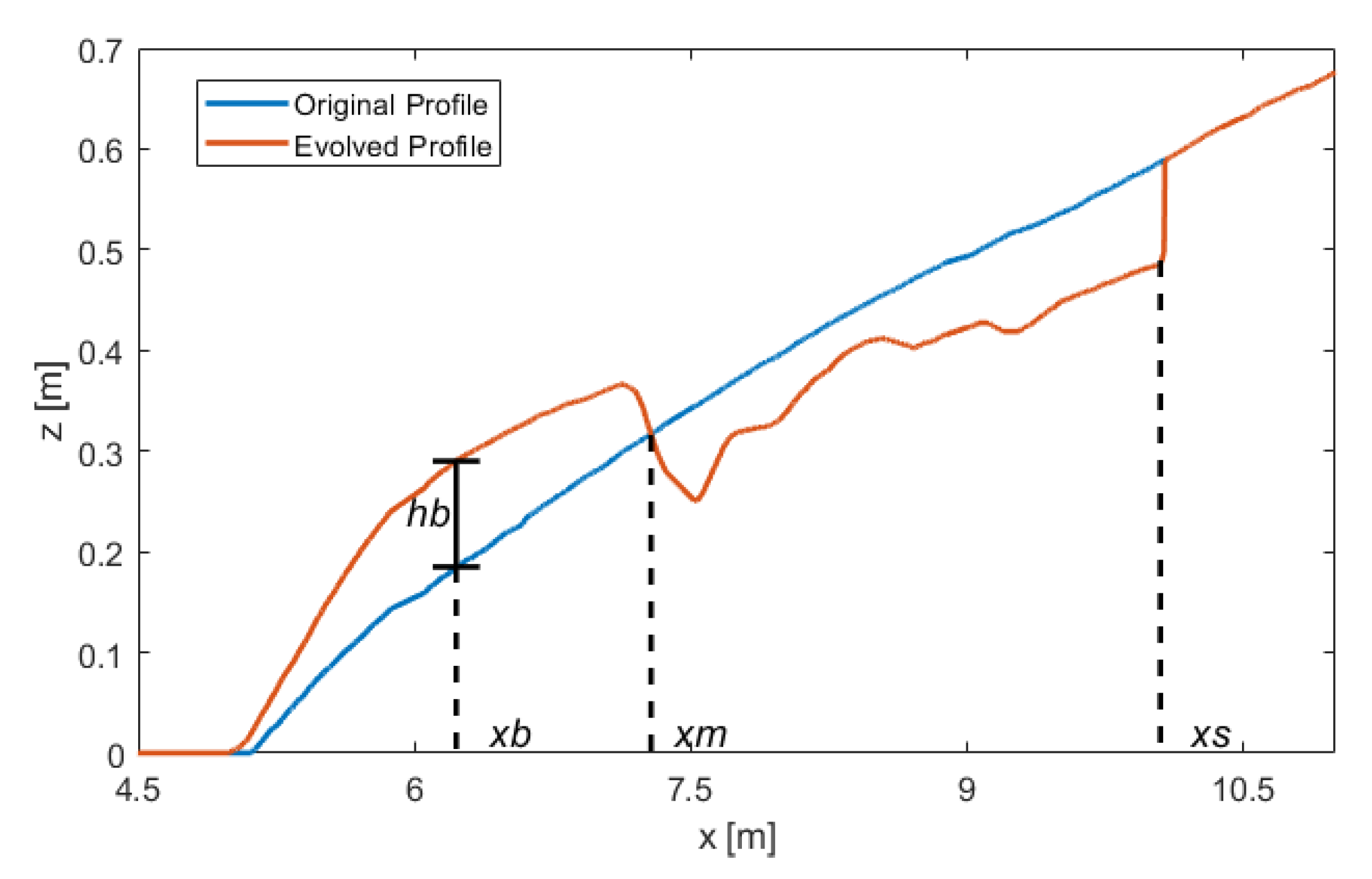
2.2.6. Dimension of the Profile Feature

During the experiment, the beach was eroded by wave attack with vertical cut, called scarp, and the eroded sediment would settle down offshore and form the deposition as sandbar, flat berm, and terrace on the profile (Figure 3). Scarps are often found on eroding coastlines, where the profile adjusts to a new dynamic equilibrium profile, e.g., nourished beach sites [66,67]. The breaker bar migrates with the increase in volume and offshore moving location. In general, scarp and breaker bar are the morphological features linked to the erosive and depositional process on the beach.

The upper and lower locations of the scarp can be found by calculating the minimum and maximum values of the second derivative of the measured profile [68]. In this study, we used this automatic recognition method assisted with visual observation, but even so the deviation may be induced by the debris from scarp slumping at some moment. The largest horizontal coordinate (xs) between the upper and lower limit is chosen as the scarp location considering the use safety. In addition, deposition on the beach is controlled primarily by its height (hb) defined as the maximum deposition height relative to the initial slope and its corresponding cross-shore location (xb).

3. Results

The experimental results were presented for regular and irregular waves respectively. For analysis on wave transformation, significant wave heights at i-th wave gauge (H_i) were normalized by dividing the incident wave height (H₀ equaling H and H_s in Table 1 for regular and irregular waves, respectively) to make direct comparison of the energy proportion. Furthermore, the rapid morphological changes were used to express the large sediment transport rates coupled to the unsteady flows and high turbulence. Then, the link was deliberated between hydrodynamics (such as wave skewness, asymmetry, and undertow) and the total transport rates.

3.1. Regular Wave Tests

3.1.1. Hydrodynamics

As regular waves propagate onshore, higher harmonics are generated due to nonlinear wave interaction in shoaling, surf and swash zones. Spectral analysis is conducted to extract the wave components of different frequencies, namely the major (of incident frequency) and generated ones (higher harmonics). For example, spectral analysis at W8, shown in Figure 4, indicated that only one extra component emerged for R1 and R2 (B-R1, B-R2, B-AR-R1, and B-AR-R2), two for R3 (B-R3 and B-AR-R3), and three for R4 and R5 (B-R4, B-AR-R4, B-R5, and B-AR-R5). Basically, wave energy transfer happened where the generated components grew, and significant wave height decreased sharply at the wave breaking location. It is found that the numbers and frequency values of the generated components are identical in B and B-AR tests under the same incident wave. For a monochromatic wave, AR cannot change the consequential wave components resulted from nonlinear transformation, but it does change the breaking point.

The proportions relative to the incident wave height are illustrated in Figure 5 in terms of significant wave heights, the 1st major- and the 2nd generated-component where B and B-AR are depicted in orange and blue, respectively. The higher order generated components (the 3rd and 4th ones in B-R4, B-R5, B-AR-R4, and B-AR-R5) are excluded in the analysis, because their total energy proportion accounts for less than 12%, which can be neglected in morphological evolution. Overall, the cross-shore distribution of wave height appears with two patterns (one for R1 and R2, and the other for R3–R5), which are changed by AR into similar pattern.

The significant wave height and wave height of the 1st major component in B tests fluctuate against the horizontal location with significant decrease from W8 for R3–R5 and small decrease for R1 and R2, which indicate that shoaling effect dominates the area of W1–W8. The remarkable increase from W8 to W9 in the energy of the 2nd component of R1 and R2 shows that the surf zone starts in the leeside of W9, while much larger proportion of the 2nd component of R3–R5 at W7 and W8 account for earlier breaking and enhanced shoaling effect offshore.

In B-AR tests, incident waves are attenuated in advance, leading to the attenuation of shoaling and breaking effect on the beach, which show as reduce and increase in the wave heights of the 1st component and 2nd component, respectively, at W4–W8. It is noted that the energy proportions of the 2nd component at W4–W8 in B-AR-R1 are much smaller than those in other B-AR tests under regular waves, which means that AR attenuates R1 by the shoaling process and bottom friction and R2–R5 mainly by breaking. In addition, significant wave heights at the seaside of AR (W1–W3) are slightly larger than those in B tests due to the reflection effect of the structure.

Furthermore, the influence of AR on wave breaking can be reflected by comparing the mean velocity and TKE at the fixed positions (ADV1 and ADV2) under the same wave climate (

Table 2. Mean velocity and TKE at ADV1 (x = 6.1 m) and ADV2 (x = 7.0 m) under regular wave climates (depth is the distance between the probe and water surface).

	Variables	ADV1				ADV2
Test Name		Depth (cm)	Mean-V (cm/s)	Mean-W (cm/s)	TKE (cm2/s2)	Dpeth (cm)	Mean-V (cm/s)	Mean-W (cm/s)	TKE (cm2/s2)
B-R1		13.5	−1.50	0.05	643	8.5	−0.64	−0.14	343
B-AR-R1		13.5	−0.37	0.05	225	8.5	−0.29	−0.14	101
B-R2		13.5	−4.74	−0.10	1999	8.5	−1.81	−0.26	754
B-AR-R2		13.5	−1.61	−0.10	943	9.0	−0.87	−0.26	407
B-R3		13.5	−4.14	−1.11	1895	9.0	−2.00	−0.71	722
B-AR-R3		13.5	−4.14	−1.11	1362	9.0	−2.00	−0.71	945
B-R4		13.5	−7.29	−2.15	6126	9.0	−8.55	−1.13	3184
B-AR-R4		13.5	−6.14	−2.15	1897	9.0	−7.41	−1.13	1194
B-R5		13.5	−14.39	−1.36	66,498	9.0	−7.90	−0.88	6929
B-AR-R5		13.5	−4.86	−1.36	68,845	9.0	−8.97	−0.88	1648

). The negative signs of mean horizontal velocity (Mean-V) and mean vertical velocity (Mean-W) indicate the offshore and downward direction respectively. Due to Mean-V directs toward offshore in all tests, only the magnitude (absolute value) is discussed. For the same regular wave, the values of Mean-W are same in B and B-AR tests. However, AR decreased the TKE by 28–76% and Mean-V by 16–75% except for R3 and R5.

The Mean-V remained unchanged after the placement of AR under wave R3, probably because the profiles in B-R3 and B-AR-R3 resembled each other near the measurement points. As for the growth in Mean-V and TKE induced by AR under R5, the explanation also refers to prevented offshore sediment transport, leading to the remarkable decrease in water depth.

3.1.2. Beach Evolution

Figure 6 shows the beach evolution under regular waves, which indicates that AR alleviates the beach erosion significantly. In all tests, the wave attack process was observed as follows: for the first several incidents, waves broke on the initial slope and eroded the beach face causing scarp; the eroded sand was suspended into the water column and carried offshore by undertow, which collided with the next incident wave, leading to large energy loss and decreased offshore current; thus, some sediment settled down and generated the sandbar with trough where the crest of the plunging breaker dropped into the water; then, after-breaking wave bores propagated onshore, ran up the slope and undercut the beach scarp by up- and back-rush.

Under the successive wave attack, the sandbar grew in sizes with a deeper erosion trough at its leeside, and migrated seaward at a decreasing rate. The scarp gradually developed and reflected the incident wave which resulted in the following avalanching. As the depth between trough and scarp increased, wave breaking would occur, possibly leading to the formation of a smaller bar. In the stable phase, the onshore bores collided with the reflected bores, which resulted in strong local turbulence promoting the scarp retreat.

Overall, beach behavior consists of the scarp and sandbar, which can basically divide the beach profile into lower and upper parts, separated by the intersection of the initial and final slopes (xm in Figure 3). The erosion and deposition can be quantified by the volume changes of the upper and lower parts, respectively.

Table 3. The final volume changes of the lower and upper parts of the evolved profile relative to the initial profile under regular waves (xm is the intersection of the initial and final slopes; V_d and V_e are the volume changes of the lower and upper parts, which are positive and negative, indicating deposition and erosion; Δxm, ΔV_d, and ΔV_e are the difference between the variables in B and B-AR tests under specific wave climate; p is the percentage of the decreased erosion volume defined as ΔV_e divided by V_e in B tests.).

Test Name	xm (m)	Vd (m3/m)	Ve (m3/m)	Test Name	xm (m)	Vd (m3/m)	Ve (m3/m)	Δxm (m)	ΔVd (m3/m)	ΔVe (m3/m)	p (%)
B-R1	8.055	0.039	−0.033	B-AR-R1	8.505	0.019	−0.019	0.450	−0.021	0.014	42
B-R2	7.640	0.080	−0.107	B-AR-R2	8.175	0.063	−0.064	0.535	−0.018	0.043	40
B-R3	7.285	0.172	−0.196	B-AR-R3	7.440	0.066	−0.089	0.155	−0.107	0.107	55
B-R4	7.290	0.257	−0.318	B-AR-R4	7.620	0.119	−0.133	0.330	−0.138	0.185	58
B-R5	6.785	0.274	−0.343	B-AR-R5	7.645	0.152	−0.167	0.860	−0.122	0.177	52

Note: The integral range of V_e is from xm and xs, and the unstable part of the reverse slope at the scarp is regarded as the erosion part before avalanching, leading to the larger magnitude of V_e than V_d.

shows the xm, volume changes relative to the original ones of lower (V_d) and upper (V_e) parts per unit long-shore length under regular waves, which can quantify the influence of AR. Comparing B and B-AR tests, beach erosion is restrained in higher elevation as xm is increased by 16–86 cm, and deposition (V_d) and erosion volumes (V_e) are reduced by 22–62% and 40–58%, respectively.

In B-R1 and B-R2, three generated bars were captured with slight sand ripples offshore. Nevertheless, the beach evolved rapidly under R3-R5 with large amounts of suspended sediment in stochastic suspension patterns. The variation of maximum deposition thickness (hb) and its location (xb) are plotted in Figure 7. The exceptional situation happened in B-R4 and B-R5, where xb rapidly moved to the toe of the initial profile, while in the other tests, hb and xb measured the bar height and location. Generally, beach evolution in B tests showed the formation of the sandbar which quickly moved offshore. Hence, the sandbar grew in height and length, causing the xb fluctuating in a very slowly reducing trend. With larger incident waves, the sandbar would increase in volume, and migrate faster toward offshore. Compared with B tests, AR reduced the hb by 2–3 cm and increased xb by 0–0.9 m under R1–R3. The beach slope between the bar-trough and scarp became a platform in B-AR-R4 and B-AR-R5, with the horizontal length of 1.9 and 2.5 m, respectively. To sum, the sandbar forms at a higher location on the profile with lower height during the beach evolution when AR is included.

3.2. Irregular Wave Tests

3.2.1. Hydrodynamics

For irregular wave propagation along the profile of B or B-AR shown in Figure 8, wave heights of full, high, or low frequency motions vary in the cross-shore patterns with different proportion magnitude and trend. On basis of the three panels in the same row, variation in wave spectra has characteristics of energy transformation from peak frequency to higher and lower frequency domain, especially the enhancement of low frequency ones at W7–W9.

In B-J1 and B-J2, significant wave height (H_s, shown as orange triangle in Figure 8) presented a fluctuating growth trend with the maximum value at W9, while in B-J3, B-J4, and B-J5, this growth trend ended at W8 and turned to the minimum at W9. The wave height of high frequency domains (H_short, gray triangle) changed in the same way as H_s. However, the cross-shore distribution of the wave height of low frequency domains (H_long, purple triangle) varied for different incident waves, and B tests under R3-R5 shared a similar general feature.

In B-AR tests, H_s (shown as blue circle in Figure 8) at W1 and W2 basically remained the same as in the corresponding B tests, while H_s was significantly reduced from W4 to W6. As waves propagated passing AR, H_s maintained at a relatively constant value at W6–W9 in B-AR tests under J3–J5, while it slightly grew from W8 to W9 in B-AR-J1 and B-AR-J2. This trend is also found in the distribution of H_short (green circle in Figure 8). Compared with B tests, H_long (yellow circle in Figure 8) was generally decreased in B-AR-J1 and B-AR-J2, but under J3–J5 H_long was increased offshore the AR (W1–W3) and reduced on the beach (W7–W9). In summary, AR changes the cross-shore transformation of H_s and H_short into one stable pattern, while the cross-shore pattern of H_long in B-AR tests depends on the incident wave.

Furthermore, the influence of AR on the velocity was summarized in

Table 4. Mean velocity and TKE at ADV1 (x = 6.1 m) and ADV2 (x = 7.0 m) under irregular wave climates (depth is distance between the probe and water surface).

	Variables	ADV1				ADV2
Test Name		Depth (cm)	Mean-V (cm/s)	Mean-W (cm/s)	Depth (cm)	Mean-V (cm/s)	Mean-V (cm/s)	Depth (cm)	Mean-V (cm/s)
B-J1		13.5	−0.27	−0.01	171	9.0	−0.47	−0.08	64
B-AR-J1		13.5	−0.08	−0.01	105	9.0	−0.21	−0.08	40
B-J2		13.5	−1.95	−0.46	948	9.0	−1.25	−0.43	350
B-AR-J2		13.5	−0.29	−0.46	427	9.0	−0.00	−0.43	169
B-J3		13.5	−2.95	1.48	45,581	9.0	−5.42	−1.48	1156
B-AR-J3		13.5	−2.02	1.48	29,650	9.0	−1.79	−1.48	406
B-J4		13.5	−3.29	1.15	105,110	9.0	−9.16	−1.67	2365
B-AR-J4		13.5	−3.05	1.15	77,640	9.0	−2.79	−1.67	638
B-J5		13.5	−0.95	2.49	10,5270	9.0	−6.38	−1.17	4920
B-AR-J5		13.5	−1.65	2.49	87,411	9.0	−3.55	−1.17	1479

for irregular waves. At ADV1, AR decreased the TKE by 17–73% and the offshore directed Mean-V by 7–99%, except for J5, while Mean-W remained same as in B tests. Similarly, TKE and Mean-V at ADV2 were reduced by 38–73% and 44–99% with Mean-W unchanged. Additionally, larger Mean-V at ADV1 in B-AR-J5 than B-J5 results from the smaller local water depth in B-J5.

3.2.2. Beach Evolution

Beach evolution under the irregular waves (J1–J5) went through the same process as in tests under regular waves (Section 3.1.2), leading to smoother final profiles without obvious bar and trough (Figure 9), probably due to the wider breaking zone relative to regular incident waves. It is noteworthy that scarps in B test (left panels of Figure 9) have approximately the same location under irregular and regular waves with the same wave parameters. While in B-AR tests (right panels of Figure 9), final scarp locations were basically at lower position under irregular waves than under the corresponding regular waves, indicating more attenuation by AR on irregular wave run up.

In addition,

Table 5. The final volume changes of the lower and upper parts of the evolved profile relative to the initial profile under irregular waves (xm is the intersection of the initial and final slopes; V_d and V_e are the volume changes of the lower and upper parts, which are positive and negative, indicating deposition and erosion; Δxm, ΔV_d, and ΔV_e are the difference between the variables in B and B-AR tests under specific wave climate; p is the percentage of the decreased erosion volume defined as −ΔV_e divided by V_e in B tests.).

Test Name	xm (m)	Vd (m3/m)	Ve (m3/m)	Test Name	xm (m)	Vd (m3/m)	Ve (m3/m)	Δxm (m)	ΔVd (m3/m)	ΔVe (m3/m)	P (%)
B-J1	8.215	0.027	−0.029	B-AR-J1	8.420	0.015	−0.014	0.205	−0.012	0.015	52
B-J2	7.730	0.055	−0.079	B-AR-J2	8.365	0.040	−0.033	0.635	−0.015	0.047	59
B-J3	7.535	0.141	−0.156	B-AR-J3	7.845	0.053	−0.066	0.310	−0.088	0.091	58
B-J4	7.335	0.129	−0.148	B-AR-J4	7.940	0.061	−0.061	0.605	−0.068	0.086	58
B-J5	7.240	0.112	−0.165	B-AR-J5	7.895	0.065	−0.076	0.655	−0.048	0.088	53

illustrates the quantification of the profile change induced by AR under irregular waves. The erosion started at xm with the growth distance of 21–66 cm, and deposition (V_d) and erosion volumes (V_e) were reduced by 28–62% and 52–59%. Likewise, the sandbar developed and moved offshore faster with larger incident waves. Comparing Figure 10a,b, AR increased xb by 0.3–1.5 m, meaning deposition forming at the higher location corresponds to smaller hb by 0.5–3.3 cm.

Moreover, the dimension and location of the generated sandbars are compared with those in a large-scale flume experiment of Eichentopf et al. [69] using natural sand including the prototype grain size. The beach profile in this experiment, with slope of 1:15, consisted of well-sorted sand with relatively narrow grain size distribution (d₅₀ = 0.25 mm, d₁₀ = 0.154 mm, d₉₀ = 0.372 mm). The sandbar in the wave climate of H_s = 0.47 m and T_p = 3.7 s was found with bar height Z_bar = 0.22 m (i.e., hb in our manuscript) at the point of X_bar = −10.8 m (consistent with xb) corresponding to water depth h_bar = 0.72 m (calculated by multiplying the absolute value of X_bar by the slope of 1/15). In the wave climate of H_s = 0.53 m and T_p = 4.14 s, the bar was generated with height of Z_bar = 0.29 m at the point of X_bar = −13.4 m corresponding to h_bar = 0.89 m. In order to make the comparison, we converse the horizontal coordinate as in the Eichentopf experiment, which is conducted by subtracting the original x-value at the intersection of the still water level and slope from all horizontal coordinate (in the original system). Then, we scaled down bar height by the geometric scale of 10, i.e., hb = 0.022 m and hb = 0.029 m. These two bar height values are found with the locations of xb = −0.72 m and xb = −0.99 m, where the water depth of d = 0.072 m and d = 0.099 m (calculated by multiplying the absolute value of xb by the slope of 1/10). The depth ratios (h_bar/d) basically meet the geometric scale of 1/10, which basically supports the validity of the beach model in this study to simulate beach behavior in the prototype.

3.3. Cross-Shore Hydrodynamics and Morphodynamics

The mechanism of coupled hydrodynamics and morphodynamics is complex as interactions between motions at different scales lead to more complex sediment transport to affect morphological behavior. However, the hydrodynamics relating to sediment transport can be illustrated by parameterization analysis of wave energy and nonlinearity [70,71,72] such as wave height H_s, mean water elevation $\overline{\eta }$, wave skewness Sk, wave asymmetry Asy, and the induced undertow current $\overline{u}$. Therefore, the influence of AR is obtained by comparing these factors in B and B-AR tests. Wave R3 and J3 were selected as representatives for regular (Figure 11) and irregular waves (Figure 12). Since $\overline{u}$ is the offshore directed depth-average current, and its growth hereinafter means the growth in its absolute value.

In Figure 11 and Figure 12, H is the significant wave height in Figure 5 and Figure 8, and its great decay indicates the start of the surf zone where $\overline{\eta }$ changes from a negative to positive value, indicating wave set-down to set-up. In B-R3 (Figure 11a), H varied slightly between 0.077 m and 0.089 m at W1–W8 and decreased to 0.062 m at W9, and a similar trend was found in the cross-shore pattern of $\overline{\eta }$ with a decrease from W7 (Figure 11b). As Figure 11c shows, Sk maintained the values of 0.24–0.32 at W1–W6, suddenly decreased to −0.45 at W7, and then increased to 0.51 and 1.15 at W8 and W9, respectively. In general, Asy and $\overline{u}$ were positively correlated with H, and their values basically stayed constant at W1–W7 and increased significantly at W8 and W9 (Figure 11d,e). Given the above, W7 is the growth point for wave nonlinearity, and the breaking point is located very close to W9 where the sandbar and trough forms. As shown in Figure 11f,g, the maximum offshore-directed total sediment transport appeared at the local highest elevation on the generated sandbar (5.0 m < x < 7.3 m). Moreover, smaller underwater bars were also captured between break point and scarp (7.7 m < x < 9.2 m), which resulted from the smaller offshore-directed total sediment transport due to the weaker breaking.

For B-AR-R3, H reduced from the W3, and the wave heights at W6–W9 were 0.02–0.03 m smaller than in B-R3. $\overline{\eta }$ was positive at all wave gauges except for W2 and W4. Two positive peaks in cross-shore distribution of Sk were located at W5 and W9, and one positive maximum of Asy was captured at W6. These indicated that main wave breaking happened on the AR, and the wave breaking on the beach started at W9. As a result, AR increased $\overline{u}$ at W5 by 0.05 m/s and reduced at W9 by 0.01 m/s. Therefore, smaller offshore-directed total sediment transport results in a smaller sandbar (6.1 m < x < 7.6 m) compared with that in B-R3.

As in Figure 12, the hydrodynamic factors in B-J3 and B-AR-J3 show similar cross-shore patterns with those in B-R3 and B-AR-R3. Since wave energy of J3 is smaller than R3, the magnitude of total sediment transport driven by J3 is smaller than in the corresponding tests under R3, and weaker breaking happens on the beach. Hence, less erosion and deposition are found in the profile (Figure 12g,n), and the topography between the scarp and sandbar shows a gentle slope instead of small bars formed in B-R3 and B-AR-R3.

4. Discussion

4.1. Implications for Beach States

The concept of beach morphodynamic states [73] achieved widespread acceptance to classify the beach system on basis of complete assemblages of depositional forms and coupled hydrodynamic process signatures in the surf zone and beaches. For the micro-tidal environment, Wright and Short [73] established the relation between 3-dimensional morphology and sediment-wave parameter (Dean’s parameter H_b/w_sT) to identify beach state classified as two extremes (dissipative and highly reflective states) and four intermediate states (long-shore bar-trough, rhythmic bar and beach, transverse bar and rip, and ridge-runnel or low tide terrace). In this experiment, the changes induced by AR in the beach system, despite being cross-shore process oriented, show some implications for beach state transformation on condition of uniform long-shore.

There are studies [21,74] demonstrating the limitation in the application of Dean’s parameter, and the intermediate states can persist through a relatively wide range of Dean’s parameter [75] even in micro-tidal conditions. Moreover, the surf-scaling parameter $\epsilon$ [76] also allows the assessment of the likelihood of beach falling into dissipative, intermediate, or reflective state [77]. Jackson et al. [78] identified that inherited geological factors can appear to be more important determinants of beach morphology than contemporary dynamics.

In this study, beach morphology evolved from steep initial profile slope to final state. Therefore, surf-scaling parameter $\epsilon$ was calculated by Equation (17) for the immediately antecedent period as discriminant coefficient to analyze hydrodynamic implications for beach state. Then beach state in each test was visually categorized into one of six beach states on the basis of the observed morphological feature:

$$\epsilon =2{\pi }^2{H}_b/\left(g{T}^{2}ta{n}^2\beta \right),$$

(17)

where H_b is the breaker wave height, g is the acceleration of gravity, and $tan\beta$ is the beach slope. H_b was estimated according to measurement at W6 by Equation (18) [79]:

$$\frac{H_b}{H_0^{\prime }}=0.76{\left(tan\beta \right)}^{1/7}{\left(H_0^{\prime }/L_0\right)}^{-1/4},$$

(18)

where $H_0^{\prime }$ is the equivalent deep-water wave height considering refraction and diffraction, and L₀ is the deep-water wave length. In this experiment, as the wave propagation was confined as normal incidence along wave flume (perpendicular to the shore), refraction and diffraction did not happen. Therefore, the significant wave height measured at W6 was used as $H_0^{\prime }$ in Equation (18). Larger $\epsilon$ means wider surf zone and stronger turbulent dissipation of incident wave energy (Wright and Short, 1984): as long as $\epsilon <2.0-2.5$, strong reflection will continue to permit strong standing wave motion, surging breakers, and resonance, which defines the highly reflective extreme; when $\epsilon >2.5$, waves begin to plunge, dissipating energy; and dissipative state is characterized by spilling breaker occurring as $\epsilon >20$. As shown in

Table 6. The surf-scaling parameter ($\epsilon$) of all tests.

	Waves	R1	R2	R3	R4	R5	J1	J2	J3	J4	J5
Profile Type
B		8.1	7.7	9.1	9.5	8.2	8.5	10.1	12.3	12.1	10.5
B-AR		5.6	6.7	6.5	6.7	5.8	7.1	8.0	8.9	7.9	7.8

, $\epsilon$ ranges from 5.6 to 12.3, indicating plunging breaker and intermediate state in all tests, and AR decreases $\epsilon$ under the same incident wave. Hence, the morphodynamic influence of AR was analyzed by comparison between observed profile features and those in the four intermediate states.

As Figure 13a–e shows, pronounced bar and trough shape developed in B tests under regular waves. In B-R4 and B-R5, the maximum deposition (xb) rapidly moved to the toe of the initial profile and then remained there, leading to the stable bar-trough location. The quasi-equilibrium profile was achieved in B-R1 with the stable bar-trough. Therefore, beach state was identified as long-shore bar-trough ($tan\beta =0.05-0.20$) in B-R1, B-R4, andB-R5, while beach state in B-R2 and B-R3 was categorized as rhythmic bar and beach ($tan\beta =0.01-0.20$) because of bar-trough still under the migration. Comparing them with the corresponding B-AR tests, plunging breaker happened along terrace instead of bar-trough under R1 and R4 (Figure 13f,i). As a result, beach state in B-AR-R1 and B-AR-R4 was taken as low tide terrace. In addition beach states in the other B-AR tests under regular waves remained as rhythmic bar and beach for the same reason in the corresponding B tests.

Nevertheless, B and B-AR basically share the same profile feature under irregular waves. Small bars formed in B-J1 (Figure 13k) identified as long-shore bar-trough, which was changed into low tide terrace by AR (B-AR-J1 in Figure 13k). The profiles under J2 (B-J2 and B-AR-J2) kept the feature of rhythmic bar and beach topography, i.e., bar-trough under migration. The other six tests (B-J3, B-J4, B-J5, B-AR-J3, B-AR-J4, and B-AR-J5) shared characters of transverse bar and rip, where strong undertow carried the eroded sand offshore, leading to the flat deposition bar which would extend further offshore with time.

Overall, AR enhances the reflective elements and reduces the dissipative elements in beach morphodynamics in terms of cross-shore processes. It should be noted that beach states in B-AR tests still fall into the range of intermediate state, while transformation into reflective state may happen under larger waves or longer time. For more energetic waves, the erosion process will be similar with that under R5 or J5, but it will spend less time to reach the same changes and beach state. It can be inferred that larger blocks or wider layout of the AR may change the hydrodynamic environment in the lee side more significantly, leading to transformation to reflective state. Besides, a different initial beach slope may also result in a different change process of profile characteristic.

4.2. Scarp Evolution

Scarp location (xs) varies in different tests due to different surf and swash environment. Figure 14 shows its moving history with the duration time (t). The scarp retreat rate V_xs in each time interval, estimated by scarp location data (V_xs = dxs/dt), grows in the initial several minutes and then monotonically decreases with time towards zero as Figure 15 shows. In summary, scarp location (xs) recedes with time in a slowing down rate (V_xs) and ceases to move (rate being zero) when the equilibrium state is reached. Therefore, quantification of the scarp process can be decomposed into two steps regarding V_xs and xs. First, we attempted to describe the character of V_xs using the natural exponential function (exp) as below:

$$V_{xs}=a\times \exp \left(-\frac{t}{b}\right),$$

(19)

where the unit of time t is second. The fitting of Equation (19) was aimed at the steadily decreasing trend of V_xs, hence tests under R4, R5, J4, and J5 were excluded because short wave durations were insufficient to provide definitive evidence on stable stage. Second, the integral of V_xs function Equation (19) could lead to the relation between xs and time t as Equation (20):

$$xs=P2-P1\times \exp \left(-\frac{t}{b}\right),$$

(20)

where $a\times b$ is expressed by parameter P1 meaning that there are three independent parameters in this scarp model. As a consequence, curve fitting consists of two steps, i.e., firstly by Equation (19) and secondly by Equation (20), and results are shown in

Table 7. Fitting parameters of scarp model.

	Parameter	a (m/s)	b (s)	P1 (m)	P2 (m)
Test Name
B-R1		0.00054	696	0.374	9.39
B-AR-R1		0.00042	678	0.284	9.29
B-R2		0.00094	604	0.568	9.73
B-AR-R2		0.00082	591	0.482	9.73
B-R3		0.00455	265	1.208	10.02
B-AR-R3		0.00409	196	0.801	9.65
B-J1		0.00024	1701	0.403	9.43
B-AR-J1		0.00013	1410	0.188	9.20
B-J2		0.00096	691	0.662	9.74
B-AR-J2		0.00079	611	0.484	9.48
B-J3		0.00369	341	1.258	10.10
B-AR-J3		0.00262	310	0.811	9.71

Notes: P1 obtained in the second step is smaller thane $a\times b$ in the first step in each test, probably because scarp location detection induces amplified deviation in V_xs. Both P1 and e $a\times b$ are smaller in B-AR tests than in corresponding B tests. To simplify, P1 is adopted as it is acquired from the primary data (xs) with a revised by P1/b. R-square (coefficient of determination) of fitting by Equation (20) on xs data ranges from 0.92 to 1.00 with RMSE (root mean squared error) between 0.004 and 0.038.

. A relatively high fitting degree with R-square over 0.92 and RMSE below 0.04 validates the application of this scarp model to the experiment.

The underlying physics of parameters in the scarp model are explained as follows: the exponential part $\exp \left(-t/b\right)$ is non-dimensional indicator for decreasing trend, hence b has the dimension of time and P1 and P2 have the dimension of length with of a being velocity; P2 is the estimation of the scarp location at the equilibrium state corresponding to the maximum value of xs in this experimental coordinate; P1 represents the distance between the minimum and maximum value of xs, and the term of $P1\times \exp \left(-t/b\right)$ indicates how far is left before scarp to reach equilibrium; and b can indicate the time duration before equilibrium, as the distance to maximum scarp location (P2) reduces to about one third of P1 when t equals to b.

In consequence, the influence of AR on scarp process can be analyzed by comparing the scarp model parameters between B and B-AR tests under the same wave condition, and almost all the parameters are smaller in B-AR tests. The maximum scarp location P2 is basically moved seaward by AR, except for the same value under R2. Smaller b means the shorter time required to reach the equilibrium. Given the reduced a and P1, scarps in B-AR tests recede slower yet reach the maximum earlier than in corresponding B tests because of the smaller total distance P1.

Since all tests share the same sediment and initial beach slope, the variations in model parameters are purely caused by different wave run-up. The hydrodynamic impact on scarp evolution is evaluated by calculating the Pearson correlation coefficients: ($\rho \left(A,B\right)$ = $\frac{1}{N-1}{{\displaystyle \sum }}_{i=1}^N\left(\frac{A_i-{\mu }_A}{{\sigma }_A}\right)\left(\frac{B_i-{\mu }_B}{{\sigma }_B}\right)$, where $\mu$ and $\sigma$ are the mean and standard deviation of variables A and B, and N is the sample size) of model parameters (P1, P2, and b) and factors used to estimate wave run-up (offshore deep water wave height and length, the product of them, wave steepness, wave set-up, and Irribarren number). Wave set-up is the result of mean water elevation $\overline{\eta }$, and Irribarren number $\xi$ is calculated as Equation (21) with values between 0.6 and 0.9:

$$\xi =tan\beta /\sqrt{H/L},$$

(21)

where $tan\beta$ is the beach slope being initial value of 0.10. All the wave factors were calculated using measurement at W6. For irregular wave climates, the wave heights of low and high frequency components (H_long and H_short) were added into the consideration. The results are shown in

Table 8. The Pearson’s linear correlation coefficients of hydrodynamic factors and model parameters under regular waves with significant level in parentheses (H is the wave height at W6, and L is calculated by local water depth and period at W6; bold format indicates correlation coefficients with relatively low significant level meaning significant correlation).

	Factors	H	$\overline{\mathit{\eta }}$	L	H/L	$\mathit{H}\times \mathit{L}$	$\mathit{\xi }$
Cases
B-P1		0.9889 (0.03)	0.4935 (0.67)	0.9204 (0.26)	0.9848 (0.11)	0.9957 (0.06)	−0.9903 (0.09)
B-AR-P1		0.9494 (0.20)	0.9039 (0.28)	0.9788 (0.13)	0.8828 (0.31)	0.9750 (0.14)	−0.8754 (0.32)
B-P2		0.9915 (0.08)	0.6396 (0.56)	0.9751 (0.14)	0.9385 (0.22)	0.9394 (0.05)	−0.9976 (0.20)
B-AR-P2		0.9714 (0.15)	0.9351 (0.23)	0.9920 (0.08)	0.9173 (0.26)	0.9896 (0.09)	−0.9110 (0.27)
B-b		−0.9006 (0.29)	−0.8486 (0.35)	−0.9954 (0.06)	−0.7826 (0.43)	−0.9192 (0.26)	0.8040 (0.41)
B-AR-b		−0.9994 (0.02)	−0.9878 (0.10)	−0.9969 (0.05)	−0.9793 (0.13)	−0.9981 (0.04)	0.9760 (0.14)

and

Table 9. The Pearson’s linear correlation coefficients of hydrodynamic factors and model parameters under irregular waves with significant level in parentheses (H_s is significant wave height at W6, and L_s is calculated by local water depth and peak period at W6; bold format indicates correlation coefficients with relatively low significant level meaning significant correlation).

	Factors	Hs	Hlong	Hshort	$\overline{\mathit{\eta }}$	Ls	Hs/Ls	${\mathit{H}}_{\mathit{s}}\times {\mathit{L}}_{\mathit{s}}$	$\mathit{\xi }$
Cases
B-P1		0.9873 (0.10)	0.9969 (0.05)	0.9869 (0.10)	−0.8537 (0.35)	0.8998 (0.29)	0.9930 (0.08)	0.9875 (0.10)	−0.9626 (0.17)
B-AR-P1		0.9994 (0.02)	0.9736 (0.15)	0.9992 (0.03)	0.8773 (0.32)	0.9674 (0.16)	0.9999 (0.01)	0.9995 (0.02)	−0.9950 (0.06)
B-P2		0.9998 (0.01)	0.9671 (0.16)	0.9999 (0.01)	−0.7482 (0.46)	0.9628 (0.17)	0.9982 (0.04)	0.9998 (0.01)	−0.9954 (0.06)
B-AR-P2		0.9990 (0.03)	0.9524 (0.20)	0.9992 (0.02)	0.8363 (0.37)	0.9845 (0.11)	0.9957 (0.06)	0.9988 (0.03)	−0.9998 (0.01)
B-b		−0.9435 (0.22)	−0.8384 (0.37)	−0.9443 (0.21)	0.5021 (0.67)	−0.9990 (0.03)	−0.9292 (0.24)	−0.9432 (0.22)	0.9753 (0.14)
B-AR-b		−0.9691 (0.16)	−0.8701 (0.33)	−0.9702 (0.16)	−0.7068 (0.50)	−0.9996 (0.02)	−0.9557 (0.19)	−0.9680 (0.16)	0.9828 (0.12)

where significant level indicates the probability against the original hypothesis, i.e., the probability of getting a correlation as large as the observed value by random chance, when the true correlation is zero. The Pearson’s linear correlation coefficients were used as a proxy to find some clues to explain the discrepancy in scarp behavior due to the process change.

It is noteworthy that significant level (usually used threshold value of 0.05 or 0.10) in some cases is not small enough (e.g., B-AR-P1) due to limited sample size (with only three wave conditions considered for each case). As a result, analysis emphasized the comparative correlation level relative to B tests and ignored the special cases. For regular wave climates, AR increases the correlations between L and P2 and between H and b. In irregular wave tests, P2 is mostly determined by H_s and H_short, and b shows correlation only with L_s. However, P1 in B tests is highly correlated to all wave heights, while AR reduces the correlation of H_long and increases correlation of H_s and H_short, consequently leading to growth in coefficients of H_s/L_s and H_s $\times$ L_s.

In general, AR moves the scarp location seaward with a smaller retreat rate and shorter time to reach the equilibrium. Experimental results show that model parameters depend on both wave height and length for regular wave, and AR seems to improve this relatively weak correlation of them. For irregular wave condition, the length parameters (P1 and P2) and time parameter (b) are determined by total wave energy and peak period, and strong correlation between long wave and P1 disappears in the AR-protected beach. This scarp model and the effect of AR on the three parameters provide a process-based example to study the submerged structure in the view of morphodynamic evolution.

5. Conclusions

This experimental study investigated the cross-shore hydrodynamic and morphodynamic processes of beach profiles with and without AR under regular and irregular wave climates, and comparative analysis of the results revealed the influences of AR.

As regular waves propagate onshore, higher harmonics are generated due to nonlinear effects, which remain identical in the numbers and frequencies for two types of profiles under the same incident wave. Therefore, the influence of AR is to break incident wave in advance and significantly decrease wave energy that propagates onshore, but it cannot change the after-breaking fate of a monochromatic wave. Nevertheless, wave transformation varies for different frequency domains for irregular wave. In addition, this was considered by separating wave series to full, high, and low frequency motions and calculating the significant, short, and long wave heights. The cross-shore patterns of these wave heights are different in magnitude and change trend that tightly linked to wave breaking probability. With the protection of AR, significant wave height and short wave height are adjusted into one similar cross-shore distribution, while the cross-shore pattern of long wave height still depends on the incident wave to some extent.

Beach profile shows in a bar-trough type under regular waves and in a milder slope under irregular waves. AR strongly reduced the offshore sediment transport that leads to smaller erosion and deposition on the beach. The morphodynamic process is illustrated by relating the hydrodynamic factors (e.g., wave skewness, wave asymmetry, and undertow) to sediment transport. The profile changes consist of scarp retreat and sandbar migration, which are essentially driven by the offshore sediment flux due to swash erosion and accompanied with large variations of hydrodynamic factors. According to the cross-shore features proposed by Wright and Short (1984), beach states in all tests are identified as intermediate morphodynamic state. AR can enhance the reflective elements and abate the dissipative elements in morphodynamics, leading to beach state transformation, which is more significant in regular wave tests than in irregular wave tests.

The development of beach scarp resulted by wave run-up can partly reflect the morphodynamic role of AR. Scarp location can be formulated as a linear equation regarding the natural exponential of the duration time, leading to three independent fitting parameters, which are investigated by the correlation analysis in terms of hydrodynamic factors used to predict the wave run-up. The results show that AR slows down the scarp retreat rate, causing shorter time duration to a more seaward equilibrium location under the same wave climate. AR improves the relatively weaker correlation with the wave height and length during the erosion process under regular waves, while the impact of low-frequency harmonics is weakened in the AR-protected beach.

To conclude, AR reduces the incident wave energy and changes the hydrodynamic process significantly in the surf and swash zone, which enables smaller erosion and decreased shoreline retreat on the beach with the enhanced reflective elements for the beach state. This cross-shore process-based experimental research indicates that AR affects the morphodynamic environment within the surf zone to maintain the erosion control purpose, where it embodies the principles of working with natural processes, in the long term and broad overall perspective.

References

1. Luijendijk, A.; Hagenaars, G.; Ranasinghe, R.; Baart, F.; Donchyts, G.; Aarninkhof, S. The state of the world’s beaches. Sci. Rep. 2018, 8, 6641. [Google Scholar] [CrossRef] [PubMed]
2. Van Rijn, L.C. Coastal erosion and control. In Ocean & Coastal Management; Elsevier: New York, NY, USA, 2011; Volume 54, pp. 867–887. [Google Scholar]
3. McKenna, J.; Cooper, A.; O’Hagan, A.M. Managing by principle: A critical analysis of the European principles of Integrated Coastal Zone Management (ICZM). Mar. Policy 2008, 32, 941–955. [Google Scholar] [CrossRef]
4. Lamberti, A.; Archetti, R.; Kramer, M.; Paphitis, D.; Mosso, C.; Di Risio, M. European experience of low crested structures for coastal management. Coast. Eng. 2005, 52, 841–866. [Google Scholar] [CrossRef] [Green Version]
5. Ranasinghe, R.; Turner, I.L. Shoreline response to submerged structures: A review. Coast. Eng. 2006, 53, 65–79. [Google Scholar] [CrossRef]
6. Luo, S.; Cai, F.; Liu, H.; Lei, G.; Qi, H.; Su, X. Adaptive measures adopted for risk reduction of coastal erosion in the People’s Republic of China. Ocean Coast. Manag. 2015, 103, 134–145. [Google Scholar] [CrossRef]
7. Luo, S.; Liu, Y.; Jin, R.; Zhang, J.; Wei, W. A guide to coastal management: Benefits and lessons learned of beach nourishment practices in China over the past two decades. Ocean Coast. Manag. 2016, 134, 207–215. [Google Scholar] [CrossRef]
8. Gu, J.; Ma, Y.; Wang, B.; Sui, J.; Kuang, C.; Liu, J.; Lei, G. Influence of near-shore marine structures in a beach nourishment project on tidal currents in Haitan Bay, facing the Taiwan Strait. J. Hydrodyn. Ser. B 2016, 28, 690–701. [Google Scholar] [CrossRef]
9. Everts, C. Impact of Sand Retention Structures on Southern and Central California Beaches, Draft Report 2002; California Coastal Conservancy: Oakland, CA, USA, 2002.
10. Karunarathna, H.; Tanimoto, K. Numerical experiments on low-frequency fluctuations on a submerged coastal reef. Coast. Eng. 1995, 26, 271–289. [Google Scholar] [CrossRef]
11. Karunarathna, H.; Tanimoto, K. Long-period water surface fluctuations on a horizontal coastal shelf with a steep seaward face. Coast. Eng. 1996, 29, 123–147. [Google Scholar] [CrossRef]
12. Lentz, S.J.; Churchill, J.H.; Davis, K.A.; Farrar, J.T. Surface gravity wave transformation across a platform coral reef in the Red Sea. J. Geophys. Res. Oceans 2016, 121, 693–705. [Google Scholar] [CrossRef] [Green Version]
13. Masselink, G.; Tuck, M.; McCall, R.; van Dongeren, A.; Ford, M.; Kench, P. Physical and numerical modeling of infragravity wave generation and transformation on coral reef platforms. J. Geophys. Res. Oceans 2019, 124, 1410–1433. [Google Scholar] [CrossRef]
14. Sous, D.; Tissier, M.; Rey, V.; Touboul, J.; Bouchette, F.; Devenon, J.; Chevalier, C.; Aucan, J. Wave transformation over a barrier reef. Cont. Shelf Res. 2019, 184, 66–80. [Google Scholar] [CrossRef] [Green Version]
15. Ning, Y.; Liu, W.; Zhao, X.; Zhang, Y.; Sun, Z. Study of irregular wave run-up over fringing reefs based on a shock-capturing Boussinesq model. Appl. Ocean Res. 2019, 84, 216–224. [Google Scholar] [CrossRef]
16. Yao, Y.; He, W.; Du, R.; Jiang, C. Study on wave-induced setup over fringing reefs in the presence of a reef crest. Appl. Ocean Res. 2017, 66, 164–177. [Google Scholar] [CrossRef]
17. Yao, Y.; Zhang, Q.; Chen, S.; Tang, Z. Effects of reef morphology variations on wave processes over fringing reefs. Appl. Ocean Res. 2019, 82, 52–162. [Google Scholar] [CrossRef]
18. Costa, M.B.S.F.; Araújo, M.; Araújo, T.C.M.; Siegle, E. Influence of reef geometry on wave attenuation on a Brazilian coral reef. Geomorphology 2016, 253, 318–327. [Google Scholar] [CrossRef]
19. Spalding, M.D.; Ruffo, S.; Lacambra, C.; Meliance, I.; Hale, L.Z.; Shepard, C.C.; Beck, M.W. The role of ecosystems in coastal protection: Adapting to climate change and coastal hazards. Ocean Coast. Manag. 2014, 90, 50–57. [Google Scholar] [CrossRef]
20. Ferrario, F.; Beck, M.W.; Storlazzi, C.D.; Micheil, F.; Shepard, C.C.; Airoldi, L. The effectiveness of coral reefs for coastal hazard risk reduction and adaptation. Nat. Commun. 2014, 5, 3794. [Google Scholar] [CrossRef]
21. Sanderson, P.G.; Eliot, I. Compartmentalisation of beachface sediments along the southwestern coast of Australia. Mar. Geol. 1999, 1, 145–164. [Google Scholar] [CrossRef]
22. De Alegria-Arzaburu, A.R.D.; Mariño-Tapia, I.; Enriquez, C.; Silva, R.; González-Leija, M. The role of fringing coral reefs on beach morphodynamics. Geomorphology 2013, 198, 69–83. [Google Scholar] [CrossRef]
23. Reguero, B.G.; Beck, M.W.; Agostini, V.N.; Kramer, P.; Hancock, B. Coral reefs for coastal protection: A new methodological approach and engineering case study in Grenada. J. Environ. Manag. 2018, 210, 146–161. [Google Scholar] [CrossRef] [PubMed]
24. López, I.; Tinoco, H.; Aragonés, L.; García-Barba, J. The multifunctional artificial reef and its role in the defence of the Mediterranean coast. Sci. Total Environ. 2016, 550, 910–923. [Google Scholar] [CrossRef] [PubMed]
25. Lee, M.O.; Otake, S.; Kim, J.K. Transition of artificial reefs (ARs) research and its prospects. Ocean Coast. Manag. 2018, 154, 55–65. [Google Scholar] [CrossRef]
26. Folpp, H.R.; Schilling, H.T.; Clark, G.F.; Lowry, M.B.; Maslen, B.; Gregson, M.; Suthers, I.M. Artificial reefs increase fish abundance in habitat-limited estuaries. J. Appl. Ecol. 2020, 57, 1752–1761. [Google Scholar] [CrossRef]
27. Kim, D.; Woo, J.; Yoon, H.S.; Na, W.B. Wake lengths and structural responses of Korean general artificial reefs. Ocean Eng. 2014, 92, 83–91. [Google Scholar] [CrossRef]
28. Baine, M. Artificial reefs: A review of their design, application, management and performance. Ocean Coast. Manag. 2001, 44, 3–4, 241–259. [Google Scholar] [CrossRef]
29. Lima, J.S.; Zalmon, I.R.; Love, M. Overview and trends of ecological and socioeconomic research on artificial reefs. Mar. Environ. Res. 2019, 145, 81–96. [Google Scholar] [CrossRef]
30. Jordan, L.K.B.; Gilliam, D.S.; Spieler, R.E. Reef fish assemblage structure affected by small-scale spacing and size variations of artificial patch reefs. J. Exp. Mar. Biol. Ecol. 2005, 326, 170–186. [Google Scholar] [CrossRef]
31. Moschella, P.S.; Abbiati, M.; Aberg, P.; Airoldi, L.; Anderson, J.M.; Bacchiocchi, F.; Bulleri, F.; Dinesen, G.E.; Frost, M.; Gacia, E.; et al. Low-crested coastal defence structures as artificial habitats for marine life: Using ecological criteria in design. Coast. Eng. 2005, 52, 1053–1071. [Google Scholar] [CrossRef]
32. Piazza, B.P.; Banks, P.D.; Peyre, M.K.L. The Potential for Created Oyster Shell Reefs as a Sustainable Shoreline Protection Strategy in Louisiana. Restor. Ecol. 2005, 13, 8. [Google Scholar] [CrossRef]
33. Harris, L.E. Submerged Reef Structures for Beach Erosion Control. In Proceedings of the Coastal Structures 2003; Coastal Structures: Portland, OR, USA, 2003; pp. 1155–1163. [Google Scholar]
34. Borsje, B.W.; van Wesenbeeck, B.K.; Dekker, F.; Paalvast, P.; Bouma, T.J.; van Katwijk, M.M.; de Vries, M.B. How ecological engineering can serve in coastal protection. Ecol. Eng. 2011, 37, 113–122. [Google Scholar] [CrossRef]
35. Srisuwan, C.; Rattanamanee, P. Modeling of Seadome as artificial reefs for coastal wave attenuation. Ocean Eng. 2015, 103, 198–210. [Google Scholar] [CrossRef]
36. Raineault, N.A.; Trembanis, A.C.; Miller, D.C.; Capone, V. Interannual changes in seafloor surficial geology at an artificial reef site on the inner continental shelf. Cont. Shelf Res. 2013, 58, 67–78. [Google Scholar] [CrossRef]
37. Duarte Nemes, D.; Criado-Sudau, F.F.; Gallo, M.N. Beach morphodynamic response to a submerged reef. Water 2019, 11, 340. [Google Scholar] [CrossRef] [Green Version]
38. Chadwick, A.; Fleming, C.; Reeve, D.E. Coastal Engineering: Processes, Theory and Design Practice; Spon Press: London, UK, 2004. [Google Scholar]
39. Nwogu, O.; Demirbilek, Z. Infragravity wave motions and runup over shallow fringing reefs. J. Waterway Port Coast. Ocean Eng. 2010, 136, 295–305. [Google Scholar] [CrossRef]
40. Alsina, J.M.; Cáceres, I. Sediment suspension events in the inner surf and swash zone. Measurements in large-scale and high-energy wave conditions. Coast. Eng. 2011, 58, 657–670. [Google Scholar] [CrossRef]
41. Pomeroy, A.W.M.; Lowe, R.J.; Van Dongeren, A.R.; Ghisalberti, M.; Bodde, W.; Roelvink, D. Spectral wave-driven sediment transport across a fringing reef. Coast. Eng. 2015, 98, 78–94. [Google Scholar] [CrossRef] [Green Version]
42. Baldock, T.E.; Birrien, F.; Atkinson, F.; Shimamoto, T.; Wu, S.; Callaghan, D.P.; Nielsen, P. Morphological hysteresis in the evolution of beach profiles under sequences of wave climates—Part 1: Observations. Coast. Eng. 2017, 128, 92–105. [Google Scholar] [CrossRef] [Green Version]
43. Rocha, M.V.L.; Michallet, H.; Silva, P.A. Improving the parameterization of wave nonlinearities—The importance of wave steepness, spectral bandwidth and beach slope. Coast. Eng. 2017, 121, 77–89. [Google Scholar] [CrossRef]
44. Kuang, C.; Mao, X.; Gu, J.; Niu, H.; Ma, Y.; Yang, Y.; Qiu, R.; Zhang, J. Morphological processes of two artificial submerged shore-parallel sandbars for beach nourishment in nearshore zone. Ocean Coast. Manag. 2019, 179, 104870. [Google Scholar] [CrossRef]
45. Kuang, C.; Pan, Y.; Zhang, Y.; Liu, S.; Yang, Y.; Zhang, J.; Dong, P. Performance evaluation of a beach nourishment project at West Beach in Beidaihe, China. J. Coast. Res. 2011, 27, 769–783. [Google Scholar]
46. Pan, Y.; Kuang, C.; Chen, Y.; Yin, S.; Yang, Y.; Yang, Y.; Zhang, J.; Qiu, R.; Zhang, Y. A comparison of the performance of submerged and detached artificial headlands in a beach nourishment project. Ocean Eng. 2018, 159, 295–304. [Google Scholar] [CrossRef]
47. Mao, X. Study on Responses of Dynamic Environment on Beach Nourishment in Beidaihe, China; Tongji University: Shanghai, China, 2016. [Google Scholar]
48. Grasso, F.; Michallet, H.; Barthélemy, E. Sediment transport associated with morphological beach changes forced by irregular asymmetric, skewed waves. J. Geophys. Res. Oceans 2011, 116, C03020. [Google Scholar] [CrossRef] [Green Version]
49. Berni, C.; Barthélemy, E.; Michallet, H. Surf zone cross-shore boundary layer velocity asymmetry and skewness: An experimental study on a mobile bed. J. Geophys. Res. Oceans 2013, 118, 2188–2200. [Google Scholar] [CrossRef]
50. Soulsby, R. Dynamics of Marine Sands: A Manual for Practical Applications; Thomas Telford Publishing: London, UK, 1997. [Google Scholar]
51. Dean, R.; Dalrymple, R. Coastal Processes with Engineering Applications; Cambridge University Press: Cambridge, UK, 2002; p. 487. [Google Scholar]
52. Van Rijn, L.C. Principles of Sediment Transport in Rivers, Estuaries and Coastal Seas; Aqua Publications: Amsterdam, The Netherlands, 1993. [Google Scholar]
53. Ma, Y.; Kuang, C.; Han, X.; Dong, B. Wave Attenuation Mechanism of the Artificial Reef in Beidaihe, China. In Proceedings of the 28th International Ocean and Polar Engineering Conference, Sapporo, Japan, 10–15 June 2018. [Google Scholar]
54. Ma, Y.; Kuang, C.; Han, X.; Zhu, L. Experimental investigation on Regular Wave Process through an Artificial Reef. In Proceedings of the 12th ISOPE Pacific/Asia Offshore Mechanics Symposium, Jeju Island, Korea, 14–17 October 2018. [Google Scholar]
55. Herbers, T.H.C.; Elgar, S.; Guza, R.T.; O’Reilly, W.C. Infragravity-frequency (0.005–0.05 Hz) motions of the shelf. II: Free waves. J. Phys. Oceanogr. 1995, 25, 1063–1080. [Google Scholar] [CrossRef] [Green Version]
56. De Bakker, A.T.M.; Tissier, M.E.S.; Ruessink, B.G. Shoreline dissipation of infragravity waves. Cont. Shelf Res. 2014, 72, 73–82. [Google Scholar] [CrossRef]
57. Rijnsdrop, D.; Smit, P.; Zijlema, M. Non-hydrostatic modeling of infragravity waves under laboratory conditions. Coast. Eng. 2014, 85, 30–42. [Google Scholar] [CrossRef]
58. Elgar, S.; Gallagher, E.L.; Guza, R.T. Nearshore sandbar migration. J. Geophys. Res. 2001, 106, 11623–11627. [Google Scholar] [CrossRef]
59. Watanabe, A.; Sato, S. A sheet-flow transport rate formula for asymmetric, forward-leaning waves and currents. In Proceedings of the 29th International Conference on Coastal Engineering, Lisbon, Portugal, 19–24 September 2004; Volume 2, pp. 1703–1714. [Google Scholar]
60. Michallet, H.; Cienfuegos, R.; Barthélemy, E.; Grasso, F. Kinematics of waves propagating and breaking on a barred beach. Eur. J. Mech. B/Fluids 2011, 30, 624–634. [Google Scholar] [CrossRef]
61. Nielsen, P.; Callaghan, D.P. Shear stress and sediment transport calculations for sheet flow under waves. Coast. Eng. 2003, 47, 347–354. [Google Scholar] [CrossRef]
62. Dally, W.R.; Brown, C.A. A modelling investigation of the breaking wave roller with application to cross-shore currents. J. Geophys. Res. 1995, 110, 24873–24883. [Google Scholar] [CrossRef]
63. Mori, N.; Suzuki, T.; Kakuno, S. Noise of Acoustic Doppler Velocimeter data in bubbly flows. J. Eng. Mech. 2007, 133, 122–125. [Google Scholar] [CrossRef]
64. Goring, D.G.; Nikora, V.I. Despiking acoustic Doppler velocimeter data. J. Hydraul. Eng. 2002, 128, 117–126. [Google Scholar] [CrossRef] [Green Version]
65. Ting, F.C.K. Wave and Turbulence Characteristics in Narrow-band Irregular Breaking Waves. In Proceedings of the 4th International Symposium on Ocean Wave Measurement and Analysis, San Francisco, CA, USA, 2–6 September 2001; pp. 1052–1061. [Google Scholar]
66. De Schipper, M.A.; Darnall, J.; De Vries, S.; Reniers, A.J.H.M. Beach scarp evolution and prediction. In Proceedings of the Coastal Symposium, Kohala Coast, HI, USA, 4–8 January 2017; pp. 791–800. [Google Scholar]
67. Van Bemmelen, C.W.T. Beach Scarp Morphodynamics: Formation, Migration and Destruction. Master’s Thesis, Delft University of Technology, National University of Singapore, Singapore, 2018. [Google Scholar]
68. Alegria-Arzaburu, A.R.D.; Mariño-Tapia, I.; Silva, R.; Pedrozo-Acuña, A. Post-nourishment beach scarp morphodynamics. In Proceedings of the 12th International Coastal Symposium, Plymouth, UK, 9–12 April 2013; pp. 576–581. [Google Scholar]
69. Eichentopf, S.; Cáceres, I.; Alsina, J.M. Breaker bar morphodynamics under erosive and accretive wave conditions in large-scale experiments. Coast. Eng. 2018, 138, 36–48. [Google Scholar] [CrossRef] [Green Version]
70. Elfrink, B.; Hanes, D.M.; Ruessink, B.G. Parameterization and simulation of near bed orbital velocities under irregular waves in shallow water. Coast. Eng. 2006, 53, 915–927. [Google Scholar] [CrossRef]
71. Ruessink, B.G.; Ramaekers, G.; Van Rijn, L.C. On the parameterization of the free-stream non-linear wave orbital motion in nearshore morphodynamic models. Coast. Eng. 2012, 65, 56–63. [Google Scholar] [CrossRef]
72. Dong, G.; Chen, H.; Ma, Y. Parameterization of nonlinear shallow water waves over sloping bottoms. Coast. Eng. 2014, 94, 23–32. [Google Scholar] [CrossRef]
73. Wright, L.D.; Short, A.D. Morphodynamic variability of surf zones and beaches-a synthesis. Mar. Geol. 1984, 56, 93–118. [Google Scholar] [CrossRef]
74. Masselink, G.; Pattiaratchi, C.B. Seasonal changes in beach morphology along the sheltered coastline of Perth, Western Australia. Mar. Geol. 2001, 172, 243–263. [Google Scholar] [CrossRef]
75. Wright, L.D.; Short, A.D. Short-term changes in the morphodynamic states of beaches and surf zones: An empirical predictive model. Mar. Geol. 1985, 62, 339–364. [Google Scholar] [CrossRef]
76. Guza, R.T.; Inman, D.L. Edge waves and beach cusps. J. Geophys. Res. 1975, 80, 2997–3012. [Google Scholar] [CrossRef]
77. Anthony, E.J. Sediment-Wave parametric characteristic of beaches. J. Coast. Res. 1998, 14, 347–352. [Google Scholar]
78. Jackson, D.W.T.; Cooper, J.A.G.; del Rio, L. Geological control of beach morphodynamic state. Mar. Geol. 2005, 216, 297–314. [Google Scholar] [CrossRef]
79. Le Mehaute, B.; Koh, R.C.Y. On the breaking of waves arriving at an angle to the shore. J. Hydraul. Res. 1967, 5, 67–80. [Google Scholar] [CrossRef]
Figure 1. The application of AR in the beach nourishment project of West Beach in Qinhuangdao, China: (a) geographical location; (b) typical profiles before (201009) and after the project (201203); (c) the construction of AR; (d) AR at the lowest tide.
Water 12 02947 g001
Figure 2. Experimental setup: (a) side-view layout for natural beach (profile type B); (b) the AR protected beach (profile type B-AR); (c) photo of the model AR in the flume.
Water 12 02947 g002
Figure 3. Dimension of the sandbar and the scarp (xb and hb are the location and height of the bar; xm is the intersection of original and evolved profiles; xs is the location of scarp).
Water 12 02947 g003
Figure 4. Spectral analysis at wave gauge of W8 (location shown in Figure 2) in regular wave tests.
Water 12 02947 g004
Figure 5. The cross-shore distribution of characteristic wave height (Hi) relative to the incident wave height (H0) in regular wave tests (panels sorted by (ae) indicate the wave conditions from R1 to R5; for a specific wave condition, three panels from left to right, numbered 1, 2, 3, show the transformation of significant wave height, the 1st- and the 2nd-components, respectively; H0 is the model wave height in Table 1; W1–W9 are the wave gauges in Figure 2).
Water 12 02947 g005
Figure 6. Bed evolution under regular wave climates (left panels show the profile type B, and right panels show the profile type B-AR, where profiles are shown with colors changing from light to dark as time progresses; the profiles are captured in different time intervals for wave climates, which are 5 min for R1, 1 min for R2 and R3, 20 s for R4, and 10 s for R5. The green dash line rectangle in the right panel depicts the AR; the horizontal blue line represents the still water level, and the black circles are wave gauges and triangles are ADVs in Figure 2).
Water 12 02947 g006
Figure 7. Maximum deposition thickness hb and its cross-shore location xb during beach evolution under regular waves: (a) B tests; (b) B-AR tests (The values are derived from profiles in Figure 6, and hence the time intervals of the triangles or circles are 5 min for R1, 1 min for R2 and R3, 20 s for R4, and 10 s for R5).
Water 12 02947 g007
Figure 8. The cross-shore distribution of characteristic wave height (Hi) relative to the incident (H0) in irregular wave tests (panels sorted by (ae) indicate the wave conditions from J1 to J5; for a specific wave condition, three panels from left to right, numbered 1, 2, 3, show significant wave height, wave height of high and low frequency domains, respectively; H0 is the model wave height in Table 1; W1–W9 are the wave gauges in Figure 2).
Water 12 02947 g008
Figure 9. Comparison of bed profiles after the same duration under irregular (orange profile) and regular wave climates (blue profile) with the same wave parameters ((a,c,e,g,i) show the comparisons for profile type B, and (b,d,f,h,j) show the comparisons for profile type B-AR; the green dash line rectangle in the right panel depicts the AR; the horizontal blue line represents the still water level, and the black circles are wave gauges and triangles are ADVs in Figure 2).
Water 12 02947 g009
Figure 10. Maximum deposition thickness hb and its cross-shore location xb during beach evolution under irregular waves: (a) B tests; (b) B-AR tests (The time intervals of the triangles or circles are same as in Figure 7, which are 5 min for J1, 1 min for J2 and J3, 20 s for J4, and 10 s for J5).
Water 12 02947 g010
Figure 11. Cross-shore distribution of significant wave height H (a,h), mean water elevation η ¯ (b,i), wave skewness Sk (c,j), wave asymmetry Asy (d,k), undertow u ¯ (e,l), total sediment transport q s ¯ (f,m), initial (dashed) and final beach profile (solid) under wave R3. The final profiles (g,n) are the results from 20 min wave attack. The left panels (ag) show factors in B-R3, and the right panels (hn) show those in B-AR-R3. The green dash line rectangle in the right panel depicts the AR.
Water 12 02947 g011
Figure 12. Cross-shore distribution of factors (same as that in Figure 11) under wave J3. The final profiles (g,n) are the results from the 20 min wave attack. The left panels (ag) show factors in B-J3, and the right panels (hn) show those in B-AR-J3, and other details are same as in Figure 11.
Water 12 02947 g012
Figure 13. Observed beach state in: (ae) B tests in regular waves; (fj) B-AR tests in regular waves; (ko) B tests in irregular waves; (pt) B-AR tests in irregular waves (s = t a n β means the beach slope).
Water 12 02947 g013
Figure 14. The variation of the scarp position (xs) over time duration (t) (upper panels (ae) show the comparison between B and B-AR tests under regular wave conditions, and lower panels (fj) show the comparison under irregular wave conditions)
Water 12 02947 g014
Figure 15. The change of the scarp retreat rate (Vxs) over time duration (t) (upper panels (ae) show the comparison between B and B-AR tests under regular wave conditions, and lower panels (fj) show the comparison under irregular wave conditions)
Water 12 02947 g015