Evaluation of Temporal Contribution of Groundwater to a Small Lake through Analyses of Water Quantity and Quality


 ,
,  , ,
, ,
Abstract
1. Introduction
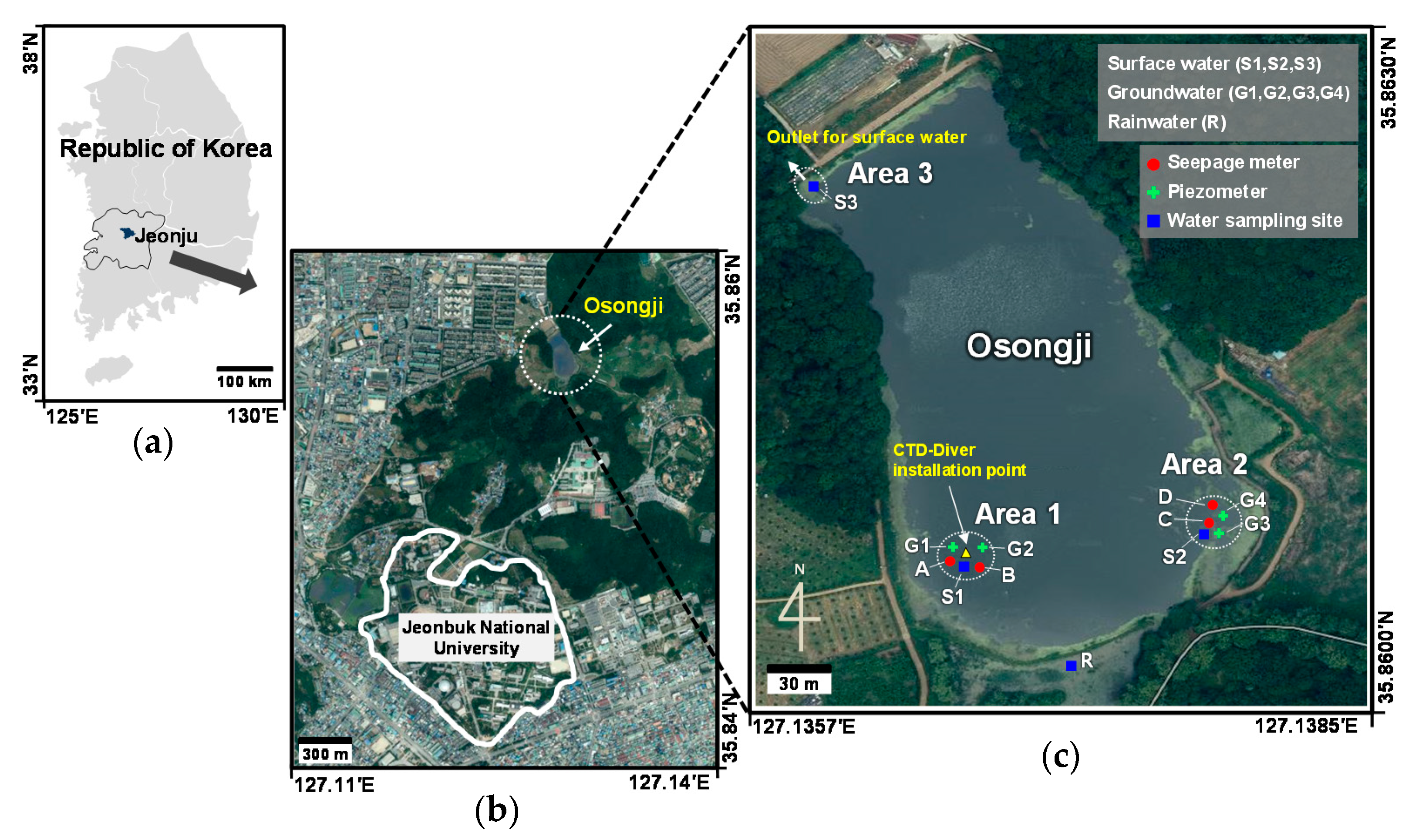
2. Study Area
3. Methods
3.1. Field Methods
3.2. Sampling and Analyses
4. Results and Discussion
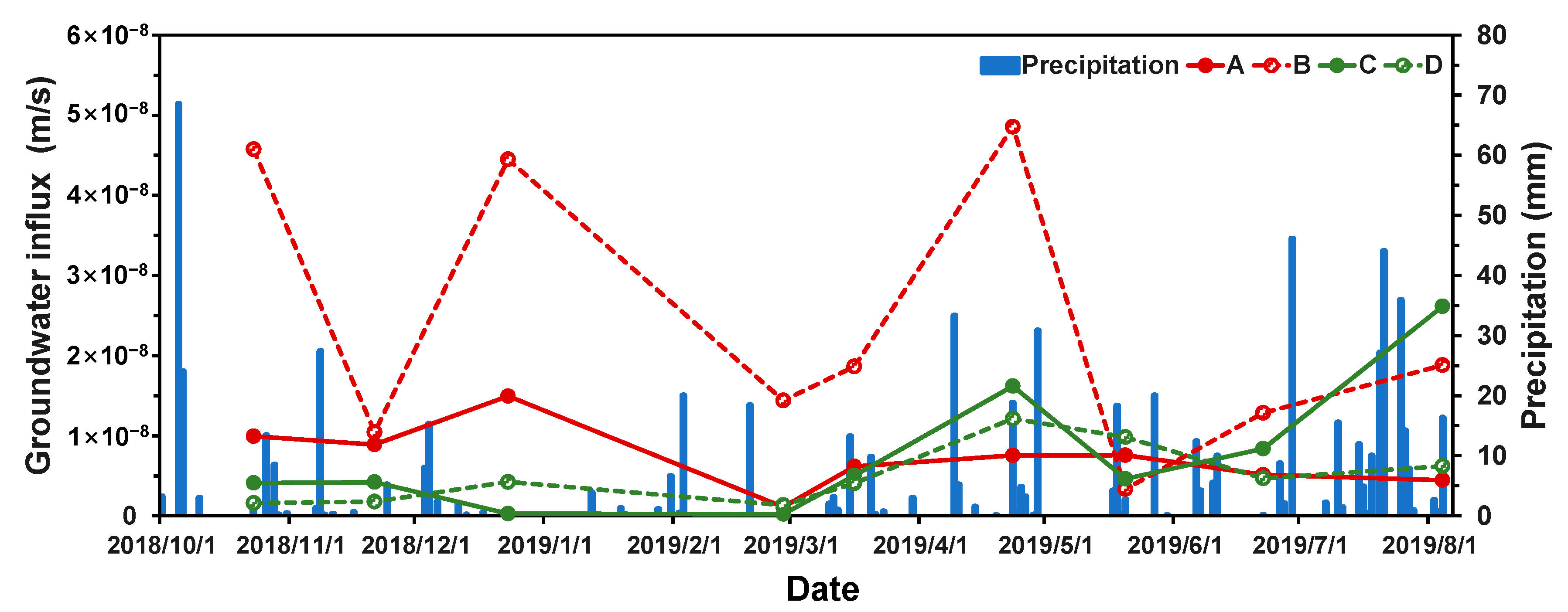
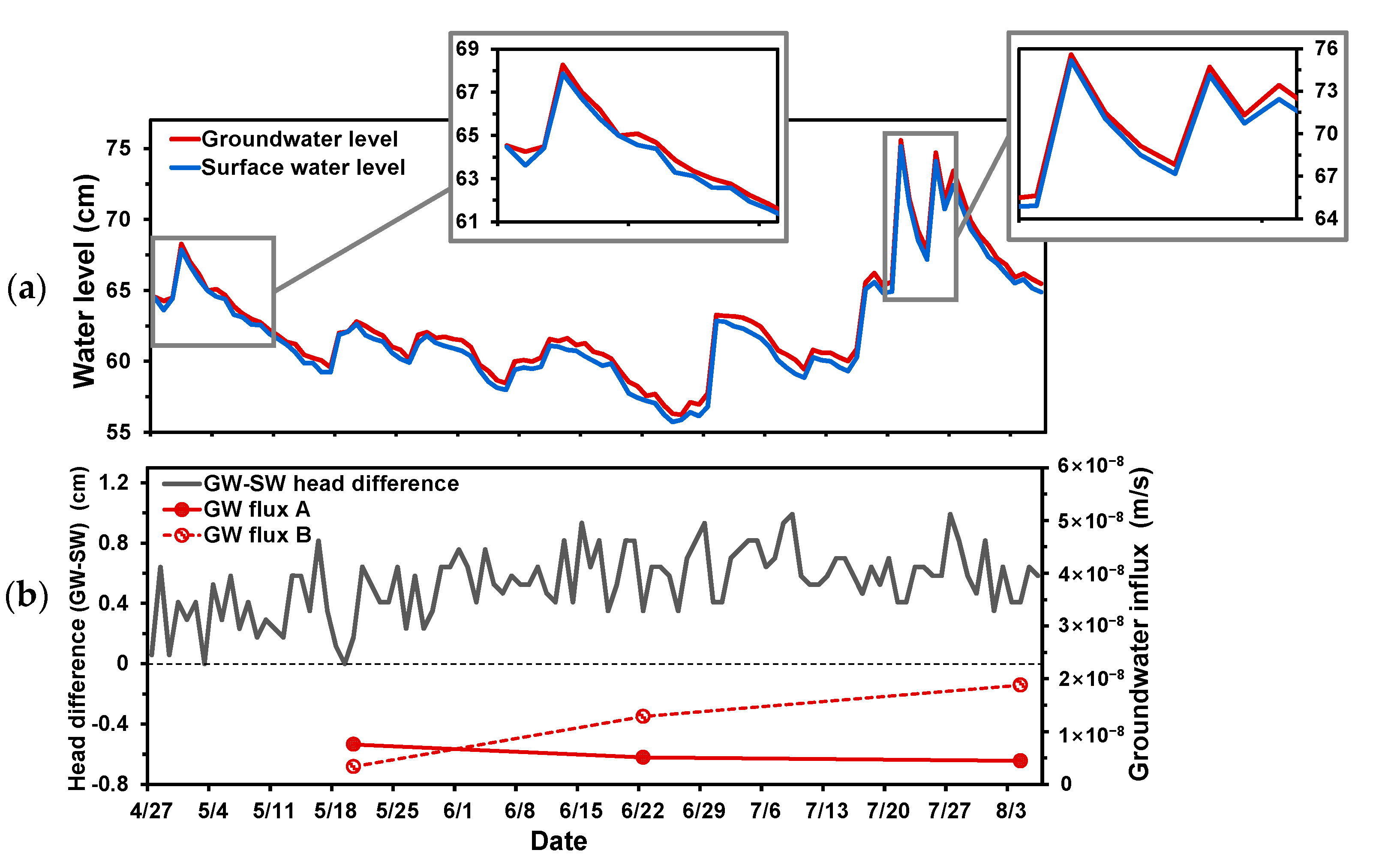
4.1. Groundwater Flux
4.2. Water Levels and Grain Size Distribution
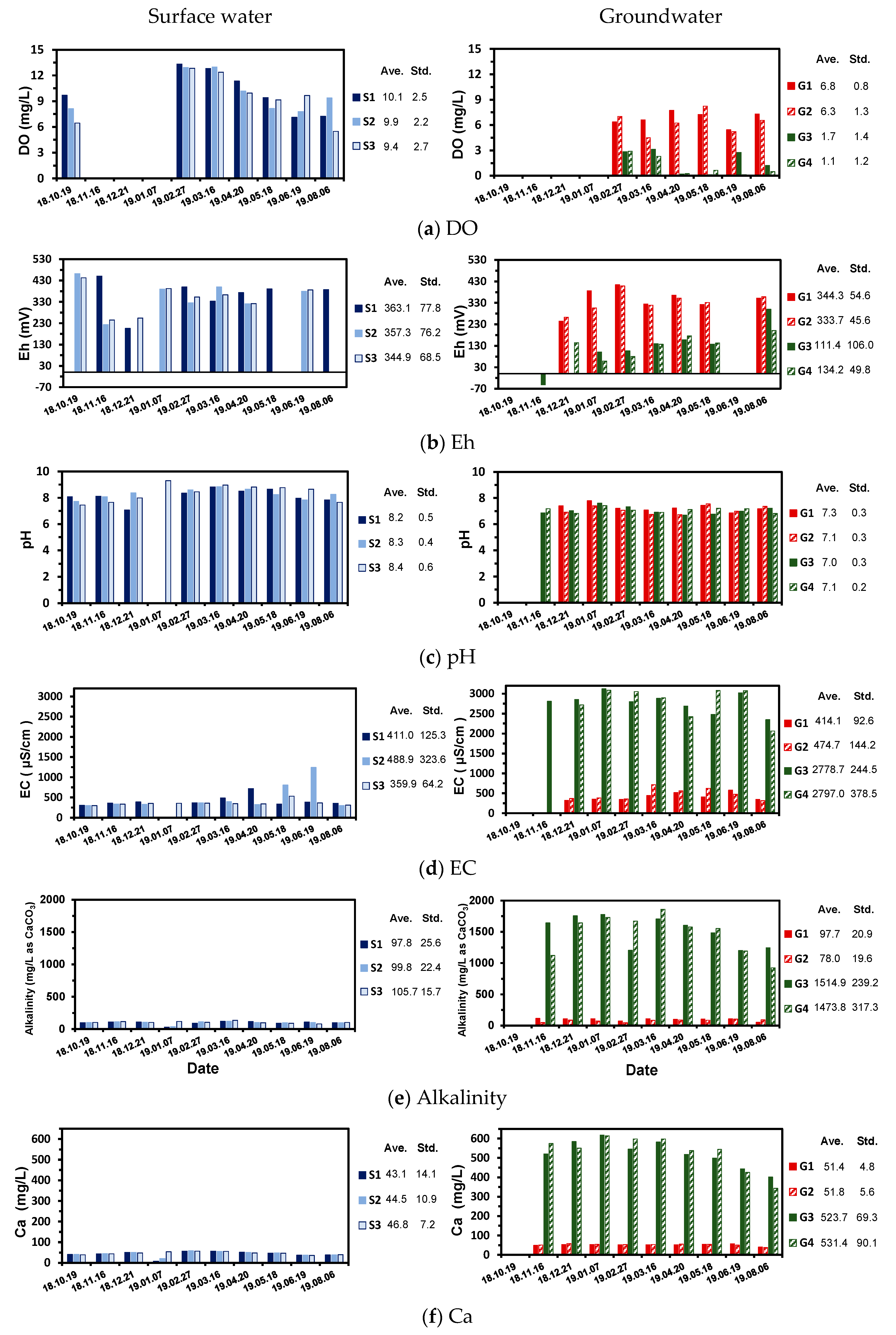
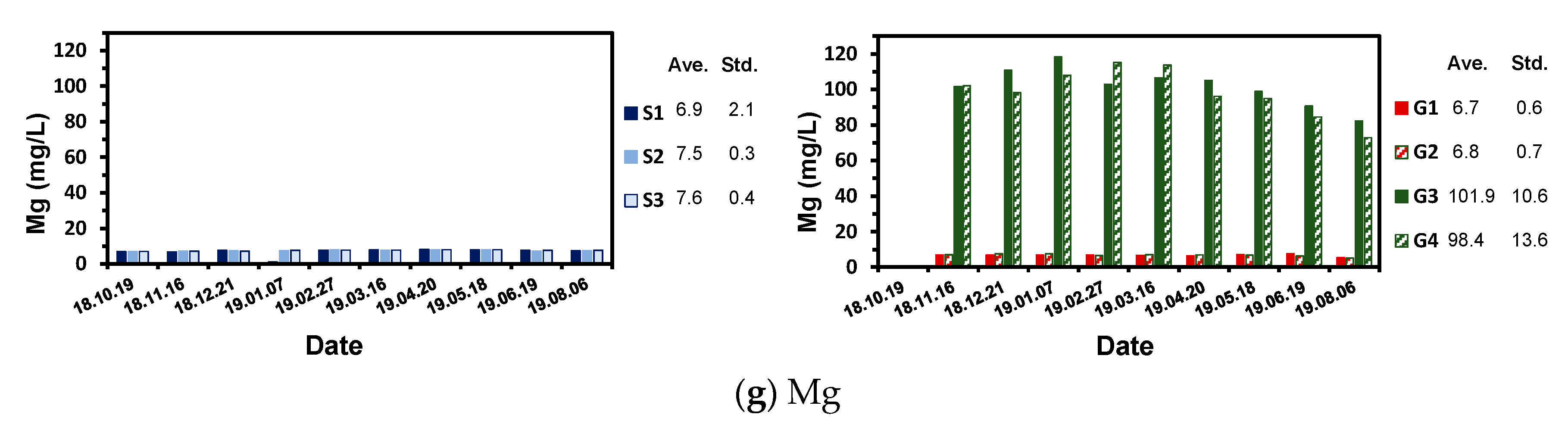
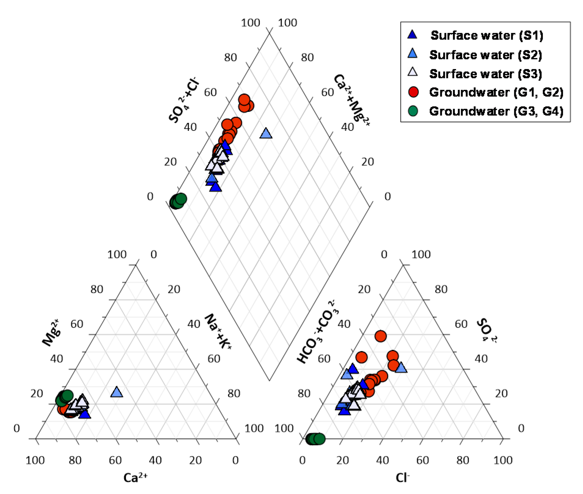
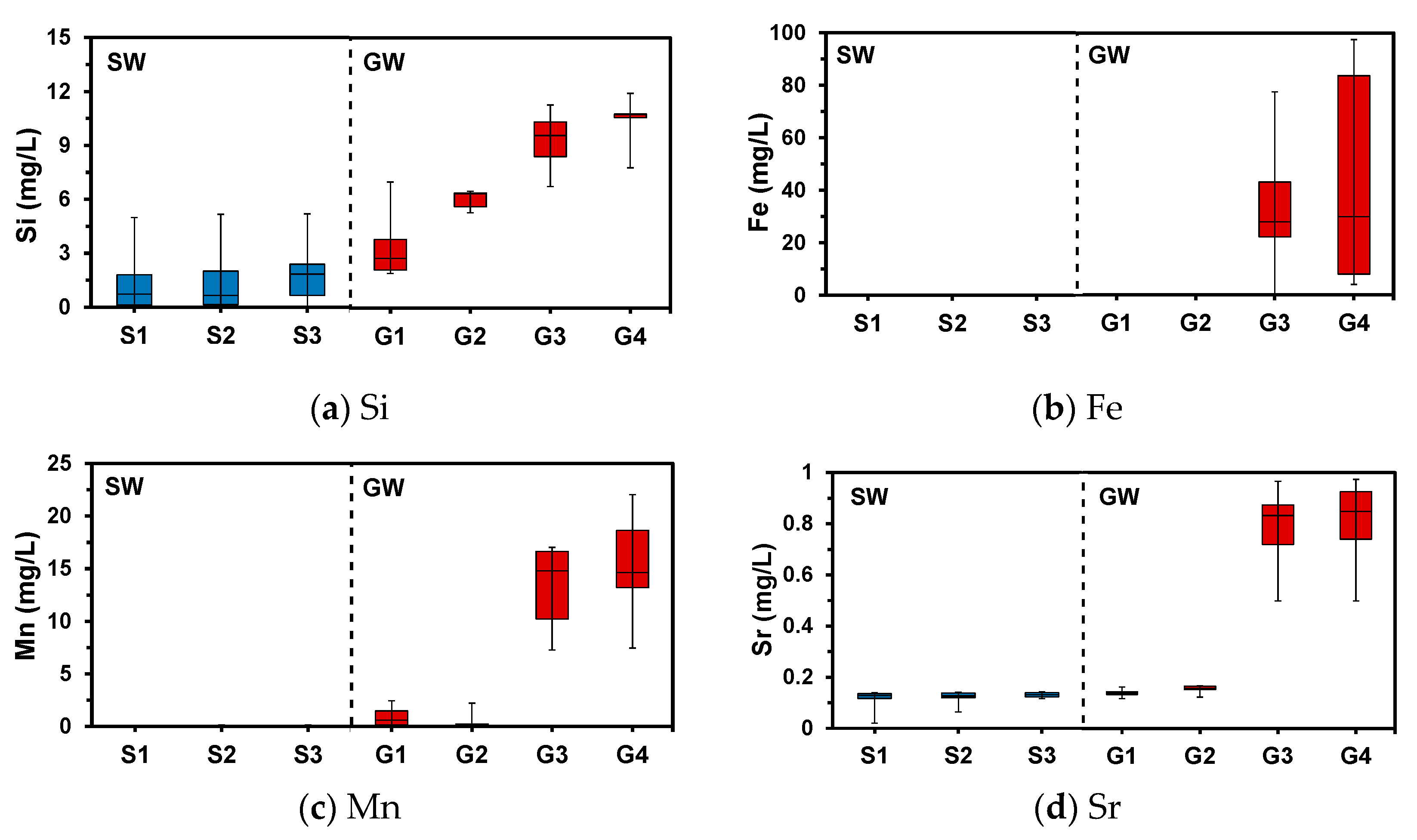
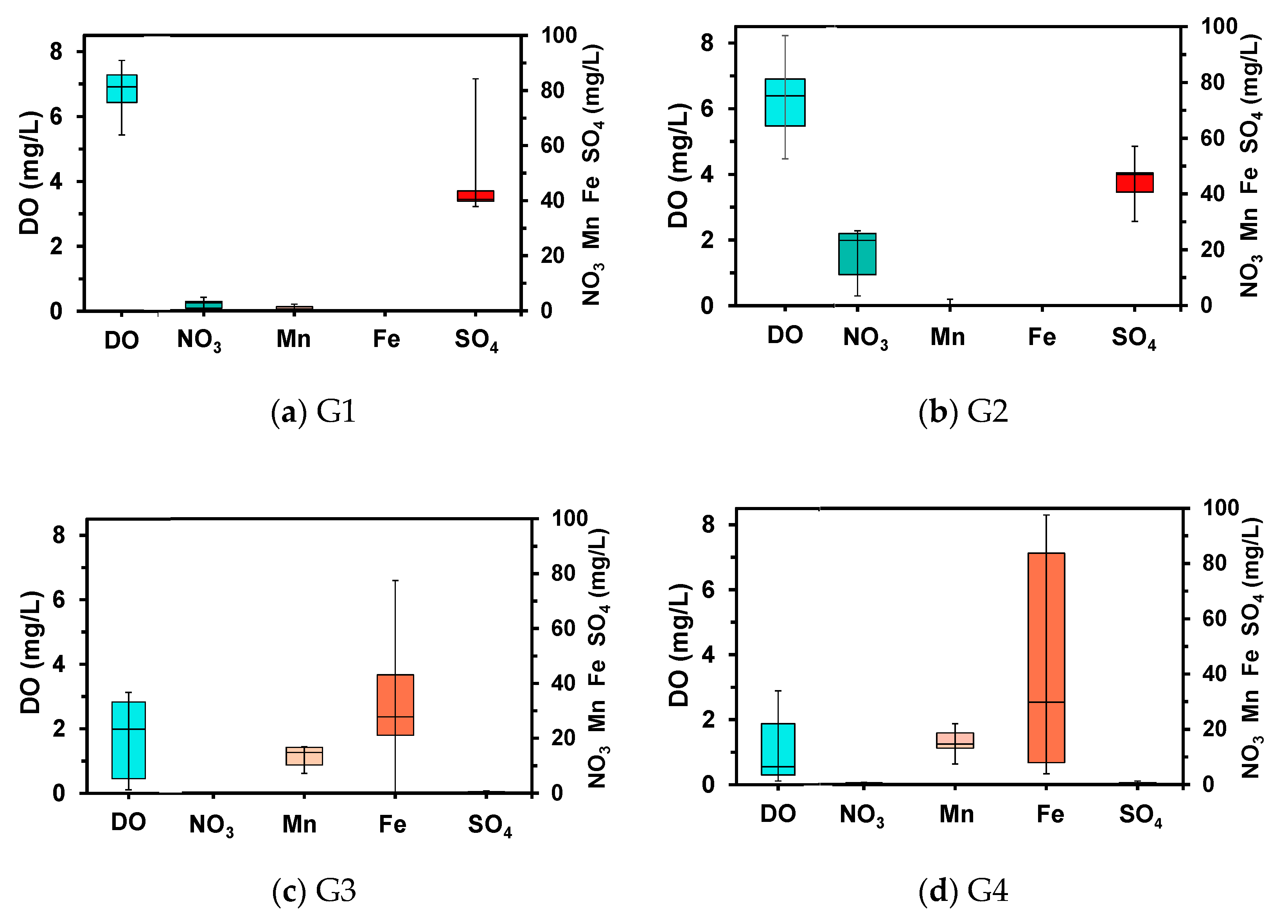
4.3. Aqueous Chemistry
4.4. Isotopic Compositions of Water Components
5. Conclusions
Supplementary Materials
Author Contributions
Funding
Conflicts of Interest
References
- Born, S.M.; Smith, S.A.; Stephenson, D.A. Hydrogeology of glacial-terrain lakes, with management and planning applications. J. Hydrol. 1979, 43, 7–43. [Google Scholar] [CrossRef]
- Winter, T.C.; Harvey, J.W.; Franke, O.L.; Alley, W.M. Ground Water and Surface Water: A Single Resource; U.S. Geological Survey (USGS): Reston, VA, USA, 1998; Volume 1139. [Google Scholar]
- Downing, J.A.; Peterka, J.J. Relationship of rainfall and lake groundwater seepage. Limnol. Oceanogr. 1978, 23, 821–825. [Google Scholar]
- Barkle, G.F.; Stenger, R.; Burgess, C.; Wall, A. Quantifying groundwater contribution to stream flow generation in a steep headwater catchment. J. Hydrol.: New Zealand 2014, 53, 23–40. [Google Scholar]
- Orlova, J.; Branfireun, B.A. Surface water and groundwater contributions to streamflow in the James Bay Lowland, Canada. Arct. Antarct. Alp. Res. 2014, 46, 236–250. [Google Scholar] [CrossRef]
- Choi, Y.H.; Park, Y.S.; Ryu, J.; Lee, D.J.; Kim, Y.S.; Choi, J.; Lim, K.J. Analysis of baseflow contribution to streamflow at several flow stations. J. Geol. Soc. Korea 2014, 30, 441–451, (In Korean with English abstract). [Google Scholar] [CrossRef][Green Version]
- Hagerthey, S.E.; Kerfoot, W.C. Groundwater flow influences the biomass and nutrient ratios of epibenthic algae in a north temperate seepage lake. Limnol. Oceanogr. 1998, 43, 1227–1242. [Google Scholar] [CrossRef]
- Rozemeijer, J.C.; Broers, H.P. The groundwater contribution to surface water contamination in a region with intensive agricultural land use (Noord-Brabant, The Netherlands). Environ. Pollut. 2007, 148, 695–706. [Google Scholar] [CrossRef]
- Shaw, G.D.; White, E.S.; Gammons, C.H. Characterizing groundwater-lake interactions and its impact on lake water quality. J. Hydrol. 2013, 492, 69–78. [Google Scholar] [CrossRef]
- Meinikmann, K.; Hupfer, M.; Lewandowski, J. Phosphorus in groundwater discharge—A potential source for lake eutrophication. J. Hydrol. 2015, 524, 214–226. [Google Scholar] [CrossRef]
- Zhu, D.; Ryan, M.C.; Sun, B.; Li, C. The influence of irrigation and Wuliangsuhai Lake on groundwater quality in eastern Hetao Basin, Inner Mongolia, China. Hydrogeol. J. 2014, 22, 1101–1114. [Google Scholar] [CrossRef]
- Kalbus, E.; Reinstorf, F.; Schirmer, M. Measuring methods for groundwater—Surface water interactions: A review. Hydrol. Earth Syst. Sci. 2006, 10, 873–887. [Google Scholar] [CrossRef]
- Lee, C.; Kim, W.; Jeen, S.-W. Analysis of water budget through measurement of groundwater flux using seepage meters at Osongji in Jeonju-si. J. Geol. Soc. Korea 2019, 55, 461–472, (In Korean with English abstract). [Google Scholar] [CrossRef]
- Lee, D.R. A device for measuring seepage flux in lakes and estuaries. Limnol. Oceanogr. 1977, 22, 140–147. [Google Scholar] [CrossRef]
- Lawrence, C.; Murdoch, L.C.; Kelly, S.E. Factors affecting the performance of conventional seepage meters. Water Resour. Res. 2003, 39, 424. [Google Scholar]
- Rosenberry, D.O. Seepage meter designed for use in flowing water. J. Hydrol. 2008, 359, 118–130. [Google Scholar] [CrossRef]
- Vogt, T.; Schneider, P.; Hahn-Woernle, L.; Cirpka, O.A. Estimation of seepage rates in a losing stream by means of fiber-optic high-resolution vertical temperature profiling. J. Hydrol. 2010, 380, 154–164. [Google Scholar] [CrossRef]
- Lee, D.R.; Cherry, J.A. A field exercise on groundwater flow using seepage meters and minipiezometers. J. Geol. Educ. 1978, 27, 6–10. [Google Scholar] [CrossRef]
- Rautio, A.; Korkka-Niemi, K. Characterization of groundwater-lake water interactions at Pyhäjärvi, a lake in SW Finland. Boreal Environ. Res. 2011, 16, 363–380. [Google Scholar]
- Chen, X.; Song, J.; Cheng, C.; Wang, D.; Lackey, S.O. A new method for mapping variability in vertical seepage flux in streambeds. Hydrogeol. J. 2009, 17, 519–525. [Google Scholar] [CrossRef]
- Brodie, R.S.; Baskaran, S.; Ransley, T.; Spring, J. Seepage meter: Progressing a simple method of directly measuring water flow between surface water and groundwater systems. Aust. J. Earth Sci. 2009, 56, 3–11. [Google Scholar] [CrossRef]
- Kim, H.; Lee, J.Y.; Park, Y.; Hyun, Y.; Lee, K.K. Groundwater and stream water exchange revealed by water chemistry in a hyporheic zone of agricultural area. Paddy Water Environ. 2014, 12, 89–101. [Google Scholar] [CrossRef]
- Klaus, J.; McDonnell, J.J. Hydrograph separation using stable isotopes: Review and evaluation. J. Hydrol. 2013, 505, 47–64. [Google Scholar] [CrossRef]
- Jung, Y.Y.; Koh, D.C.; Lee, J.; Ko, K.S. Applications of isotope ratio infrared spectroscopy (IRIS) to analysis of stable isotopic compositions of liquid water. Econ. Environ. Geol. 2013, 46, 495–508, (In Korean with English abstract). [Google Scholar] [CrossRef]
- Kim, H.; Cho, S.H.; Lee, D.; Jung, Y.Y.; Kim, Y.H.; Koh, D.C.; Lee, J. Old Water Contributions to a Granitic Watershed, Dorim-cheon, Seoul. J. Soil Groundw. Environ. 2015, 20, 34–40. [Google Scholar] [CrossRef]
- Sklash, M.G.; Farvolden, R.N. The role of ground-water in storm runoff. J. Hydrol. 1979, 43, 45–65. [Google Scholar] [CrossRef]
- Moore, R.D. Tracing runoff sources with deuterium and oxygen-88 during spring melt in a headwater catchment, southern Laurentians, Quebec. J. Hydrol. 1989, 112, 135–148. [Google Scholar] [CrossRef]
- Hatch, C.E.; Fisher, A.T.; Revenaugh, J.S.; Constantz, J.; Ruehl, C. Quantifying surface water–groundwater interactions using time series analysis of streambed thermal records: Method development. Water Resour. Res. 2006, 42, W10410. [Google Scholar] [CrossRef]
- Keery, J.; Binley, A.; Crook, N.; Smith, J.W. Temporal and spatial variability of groundwater-surface water fluxes: Development and application of an analytical method using temperature time series. J. Hydrol. 2007, 336, 1–16. [Google Scholar] [CrossRef]
- Anderson, M.P. Heat as a ground water tracer. Ground Water 2005, 43, 951–968. [Google Scholar] [CrossRef]
- Sacks, L.A.; Herman, J.S.; Konikow, L.F.; Vela, A.L. Seasonal dynamics of groundwater-lake interactions at Doñana National Park, Spain. J. Hydrol. 1992, 136, 123–154. [Google Scholar] [CrossRef]
- Anderson, E.I. Modeling groundwater–surface water interactions using the Dupuit approximation. Adv. Water Resour. 2005, 28, 315–327. [Google Scholar] [CrossRef]
- Saha, G.C.; Li, J.; Thring, R.W.; Hirshfield, F.; Paul, S.S. Temporal dynamics of groundwater-surface water interaction under the effects of climate change: A case study in the Kiskatinaw River Watershed, Canada. J. Hydrol. 2017, 551, 440–452. [Google Scholar] [CrossRef]
- Chen, X.; Shu, L. Stream-aquifer interactions: Evaluation of depletion volume and residual effects from ground water pumping. Ground Water 2002, 40, 284–290. [Google Scholar] [CrossRef] [PubMed]
- Woessner, W.W.; Sullivan, K.E. Results of seepage meter and mini-piezometer study, Lake Mead, Nevada. Ground Water 1984, 22, 561–568. [Google Scholar] [CrossRef]
- Cey, E.E.; Rudolph, D.L.; Parkin, G.W.; Aravena, R. Quantifying groundwater discharge to a small perennial stream in southern Ontario, Canada. J. Hydrol. 1998, 210, 21–37. [Google Scholar] [CrossRef]
- Choi, S.H.; Kim, S.H.; Lee, J.W.; Kim, K.J.; Oh, C.W. A study on obtaining waters to restore the water-ecosystem of Deokjin Pond in Jeonju: New paradigm for restoration of urban reservoirs. Econ. Environ. Geol. 2015, 48, 467–475, (In Korean with English abstract). [Google Scholar] [CrossRef][Green Version]
- Jo, I.; Jeen, S.-W. Measurement of groundwater-surface water exchange rates using seepage meters: A case study of Deokjin pond in Jeonju-si. J. Geol. Soc. Korea 2018, 54, 433–441, (In Korean with English abstract). [Google Scholar] [CrossRef]
- Craig, H. Isotopic variations in meteoric waters. Science 1961, 133, 1702–1703. [Google Scholar] [CrossRef]
- Wentworth, C.K. A scale of grade and class terms for clastic sediments. J. Geol. 1922, 30, 377–392. [Google Scholar] [CrossRef]
- Vukovic, M.; Soro, A. Determination of Hydraulic Conductivity of Porous Media from Grain-Size Composition; Water Resources Publications: Littleton, CO, USA, 1992. [Google Scholar]
- Appelo, C.A.J.; Postma, D. Geochemistry, Groundwater and Pollution, 2nd ed.; Balkema Publisher: Amsterdam, The Netherlands, 2005. [Google Scholar]
- Lee, J. A review on hydrograph separation using isotopic tracers. J. Geol. Soc. Korea 2017, 53, 339–346, (In Korean with English abstract). [Google Scholar] [CrossRef]
- Lee, K.S.; Lee, C.B. Oxygen and hydrogen isotopic composition of precipitation and river waters in South Korea. J. Geol. Soc. Korea 1999, 35, 73–84, (In Korean with English abstract). [Google Scholar]
- Posmentier, E.S.; Feng, X.; Zhao, M. Seasonal variations of precipitation δ18O in eastern Asia. J. Geophys. Res. Atmos. 2004, 109, D23106. [Google Scholar] [CrossRef]
- Lee, K.S.; Grundstein, A.J.; Wenner, D.B.; Choi, M.S.; Woo, N.C.; Lee, D.H. Climatic controls on the stable isotopic composition of precipitation in Northeast Asia. Clim. Res. 2003, 23, 137–148. [Google Scholar] [CrossRef]
- Lee, K.S.; Chung, J.I. Stable isotopic variation of precipitation in Pohang, Korea. Econ. Environ. Geol. 1997, 30, 321–325, (In Korean with English abstract). [Google Scholar]
- Park, Y.; Lee, K.S.; Yu, J.Y. Seasonal variations of dissolved ions and oxygen and hydrogen isotopic compositions of precipitation in Chuncheon, Korea. J. Geol. Soc. Korea 2006, 42, 283–292, (In Korean with English abstract). [Google Scholar]


| Ground Water | Average | Surface Water | Average | Rainwater a | |||||||
|---|---|---|---|---|---|---|---|---|---|---|---|
| Season | Month | ID | d18O (‰) | dD (‰) | d18O (‰), dD (‰) | ID | d18O (‰) | dD (‰) | d18O (‰), dD (‰) | d18O (‰) | dD (‰) |
| Autumn | October | G1 | N/A b | N/A b | N/A b | S1 | −7.8 | −55.1 | −7.7, −55.4 | N/A c | N/A c |
| G2 | S2 | −7.7 | −55.3 | ||||||||
| G3 | S3 | −7.7 | −55.7 | ||||||||
| G4 | |||||||||||
| November | G1 | −7.4 | −51.6 | −7.1, −46.8 | S1 | −7.4 | −53.0 | −7.4, −53.0 | −3.9 | −26 | |
| G2 | −7.5 | −52.4 | S2 | −7.4 | −53.0 | ||||||
| G3 | −6.7 | −42.4 | S3 | −7.5 | −53.1 | ||||||
| G4 | −7.1 | −44.7 | |||||||||
| Winter | December | G1 | −7.7 | −51.5 | −7.3, −47.2 | S1 | −7.3 | −51.4 | −7.4, −51.2 | N/A c | N/A c |
| G2 | −7.8 | −51.4 | S2 | −7.5 | −51.3 | ||||||
| G3 | −6.8 | −42.6 | S3 | −7.3 | −51.0 | ||||||
| G4 | −6.8 | −43.5 | |||||||||
| January | G1 | −7.3 | −50.9 | −7.1, −47.2 | S1 | N/A | N/A | −7.2, −51.0 | −4.4 | −16.3 | |
| G2 | −7.5 | −51.1 | S2 | N/A | N/A | ||||||
| G3 | −6.7 | −42.6 | S3 | −7.2 | −51.0 | ||||||
| G4 | −6.8 | −44.3 | |||||||||
| February | G1 | −7.2 | −51.8 | −7.0, −47.3 | S1 | −6.9 | −50.4 | −6.9, −50.6 | −9.8 | −76.2 | |
| G2 | −7.0 | −49.8 | S2 | −6.8 | −49.8 | ||||||
| G3 | −6.9 | −44.8 | S3 | −6.9 | −51.5 | ||||||
| G4 | −6.7 | −42.9 | |||||||||
| Spring | March | G1 | −6.8 | −50.1 | −6.8, −46.9 | S1 | −6.6 | −48.5 | −6.6, −49.0 | −7.0 | −42.8 |
| G2 | −7.2 | −50.9 | S2 | −6.6 | −49.3 | ||||||
| G3 | −6.9 | −44.2 | S3 | −6.7 | −49.2 | ||||||
| G4 | −6.5 | −42.5 | |||||||||
| April | G1 | −6.8 | −47.0 | −6.9, −44.9 | S1 | −6.0 | −43.8 | −5.9, −44.0 | 0.1 | −2.0 | |
| G2 | −7.4 | −49.8 | S2 | −5.8 | −44.0 | ||||||
| G3 | −6.6 | −40.9 | S3 | −5.9 | −44.2 | ||||||
| G4 | −6.7 | −42.0 | |||||||||
| May | G1 | −6.7 | −47.1 | −6.9, −45.7 | S1 | −5.5 | −41.9 | −5.4, −41.6 | 9.1 | 18.6 | |
| G2 | −7.2 | −49.5 | S2 | −5.4 | −41.4 | ||||||
| G3 | −6.8 | −42.4 | S3 | −5.3 | −41.6 | ||||||
| G4 | −6.9 | −43.6 | |||||||||
| Summer | June | G1 | −6.3 | −44.9 | −6.6, −44.4 | S1 | −5.1 | −39.5 | −4.8, −38.8 | −1.3 | −13.6 |
| G2 | −6.8 | −47.7 | S2 | −4.8 | −38.5 | ||||||
| G3 | −6.6 | −41.8 | S3 | −4.7 | −38.3 | ||||||
| G4 | −6.7 | −43.2 | |||||||||
| August | G1 | −6.1 | −46.1 | −6.6, −46.0 | S1 | −4.9 | −40.1 | −4.9, −40.1 | −5.4 | −39.9 | |
| G2 | −6.9 | −50.5 | S2 | −4.9 | −39.9 | ||||||
| G3 | −6.5 | −43.1 | S3 | −5.1 | −40.2 | ||||||
| G4 | −6.7 | −44.4 | |||||||||
| Slope (r2) | 7.60 (0.55) | 5.41 (0.98) | 7.05 (0.91) | ||||||||
Publisher’s Note: MDPI stays neutral with regard to jurisdictional claims in published maps and institutional affiliations. |
© 2020 by the authors. Licensee MDPI, Basel, Switzerland. This article is an open access article distributed under the terms and conditions of the Creative Commons Attribution (CC BY) license (http://creativecommons.org/licenses/by/4.0/).
Share and Cite
Kim, J.; Jeen, S.-W.; Lee, J.; Ko, K.-S.; Koh, D.-C.; Kim, W.; Jo, H. Evaluation of Temporal Contribution of Groundwater to a Small Lake through Analyses of Water Quantity and Quality. Water 2020, 12, 2879. https://doi.org/10.3390/w12102879
Kim J, Jeen S-W, Lee J, Ko K-S, Koh D-C, Kim W, Jo H. Evaluation of Temporal Contribution of Groundwater to a Small Lake through Analyses of Water Quantity and Quality. Water. 2020; 12(10):2879. https://doi.org/10.3390/w12102879
Chicago/Turabian StyleKim, Jeonga, Sung-Wook Jeen, Jeonghoon Lee, Kyung-Seok Ko, Dong-Chan Koh, Wonbin Kim, and Hojeong Jo. 2020. "Evaluation of Temporal Contribution of Groundwater to a Small Lake through Analyses of Water Quantity and Quality" Water 12, no. 10: 2879. https://doi.org/10.3390/w12102879
APA StyleKim, J., Jeen, S.-W., Lee, J., Ko, K.-S., Koh, D.-C., Kim, W., & Jo, H. (2020). Evaluation of Temporal Contribution of Groundwater to a Small Lake through Analyses of Water Quantity and Quality. Water, 12(10), 2879. https://doi.org/10.3390/w12102879