Article

Improved δ-SPH Scheme with Automatic and Adaptive Numerical Dissipation

1
Department of Civil, Geological and Mining Engineering, Polytechnique Montréal, 2900 Boulevard Edouard-Montpetit, Montréal, QC H3T 1J4, Canada
2
Group of Numerical Methods in Engineering, E.T.S.E. Camiños, Canais e Portos, Universidade da Coruña, Campus de Elviña, 15071 A Coruña, Spain
3
Arts et Métiers Institute of Technology, CNAM, LIFSE, HESAM University, 75013 Paris, France
*
Author to whom correspondence should be addressed.
Water 2020, 12(10), 2858; https://doi.org/10.3390/w12102858
Submission received: 1 September 2020 / Revised: 28 September 2020 / Accepted: 4 October 2020 / Published: 14 October 2020
(This article belongs to the Special Issue Computational Fluid Mechanics and Hydraulics)

Abstract

:
In this work we present a δ -Smoothed Particle Hydrodynamics (SPH) scheme for weakly compressible flows with automatic adaptive numerical dissipation. The resulting scheme is a meshless self-adaptive method, in which the introduced artificial dissipation is designed to increase the dissipation in zones where the flow is under-resolved by the numerical scheme, and to decrease it where dissipation is not required. The accuracy and robustness of the proposed methodology is tested by solving several numerical examples. Using the proposed scheme, we are able to recover the theoretical decay of kinetic energy, even where the flow is under-resolved in very coarse particle discretizations. Moreover, compared with the original δ -SPH scheme, the proposed method reduces the number of problem-dependent parameters.

1. Introduction

Lagrangian methods have great interest in problems with large interface deformations or with strong dynamics. The Smoothed Particle Hydrodynamics (SPH) method is one of the most widely used Lagrangian methods for the simulation of fluid flows. It was first introduced for astrophysical applications [1], and nowadays it is applied to a wide variety of problems [2,3,4]. The SPH method has some interesting properties. For example, it easily handles free-surface flows, it has interesting conservation properties and presents very small numerical dissipation connected with convection [4].
Among the SPH methods, there are different ways of including numerical dissipation [3,5]. Thus, many SPH formulations use a term of artificial numerical dissipation to stabilize the schemes which may introduce excessive dissipation. A different possibility is using Riemann-solvers, which leads to a different family of methods [6,7,8,9,10,11,12,13].
In particular, this work focuses on the δ -SPH family models [14,15,16,17] which are a variant of SPH for weakly-compressible flows. Compared with standard SPH formulations, the main advantage of this scheme is the stabilization of the scheme avoiding the occurrence of a non-physical energy flux to high-frequency modes [15].
In δ -SPH formulation, two extra diffusive terms are added, one in the continuity equation and the other in the momentum equation as a viscosity-like term. These terms are tuned through two parameters: δ for the continuity equation and α for the momentum equation. The additional dissipation introduced in the continuity equation leads to a reduction of the numerical high frequencies on the pressure field, leading to more regular distributions of particles. Thus, δ -SPH family of schemes alleviate one of the main problems of Lagrangian schemes. Thus, in SPH schemes, the Lagrangian nature of the schemes leads to non-uniform distributions of particles, specially in flow regions with high velocity gradients, which causes problems of stability and accuracy of the numerical schemes [15]. However, in some conditions with certain irregularities of the particle spatial configurations, the δ -SPH method does not prevent the tensile instability. Thus, a further improvement is presented in [15], where a particle shifting procedure is included in the δ -SPH formulation, leading to the δ + -SPH method.
Unfortunately, there is not a single and well defined value for these parameters [16], as they are problem dependent. Moreover, it was also shown that different values of parameters could lead to similar values of total dissipated energy [18]. In [16], the δ -SPH method is rewritten in terms of turbulence models, resulting in the δ -LES-SPH scheme, in such a way that δ and α are computed each time step using the Smagorinsky subgrid scale model. This method represents a great improvement for δ -SPH models since eliminates the need of ad-hoc definition of parameters for each problem. However, it is well known from grid-based methods that the use of the Smagorinsky closure model leads to excessive dissipation.
In this work, we propose a new method to define locally and automatically the value of the α parameter, to avoid the excessive dissipation caused by the classical Smagorinsky model. The δ parameter is kept fixed as suggested by [18]. Our proposal is based on the Automatic Dissipation Adjustment method (ADA), presented in [19] for low Mach computations using finite volume schemes and extended in [20] for supersonic and transonic computations. In the ADA method, the energy ratio (ER) criteria [21,22,23] are used to automatically adjust the amount of viscosity introduced by the numerical flux, increasing the numerical viscosity in those zones where the flow is under-resolved, and decreasing it in the other zones.
Our proposal for modifications to the δ -SPH scheme is based on the ADA method in a weakly compressible Lagrangian approach. Using the proposed scheme, we are able to recover the theoretical decay of kinetic energy, even where the flow is under-resolved in very coarse particle discretizations. The fundamental idea of the proposed method is somewhat similar to that presented in [24], where an additional stress term depending on the content of high-frequencies of the solution.
The paper is structured as follows. In Section 2, the governing equations are presented, and in Section 3, different δ -SPH formulations are presented, and then the new formulation is exposed. Section 4 is devoted to present some numerical tests to show the accuracy and robustness of the proposed methodology. Finally, the conclusions are drawn.

2. Governing Equations

In this work, we assume weakly compressible, Newtonian fluid flows in isothermal conditions. Under this hypothesis, the Navier–Stokes and displacement equations expressed in Lagrangian form read as
d ρ d t = ρ · u d u d t = p ρ + ν 2 u + g d r d t = u
where d ( . ) d t represents the material derivative following an infinitesimal fluid element (particle). ∇ is the nabla operator, ρ , p, u = ( u , v ) , r , ν and g represent density, pressure, velocity vector, position vector, kinematic viscosity and the gravity acceleration, respectively.
Since the fluid is considered as weakly-compressible, the density fluctuations are supposed to be very small and a linear state equation is assumed [25]
p = c 0 2 ( ρ ρ 0 )
where c 0 is the speed of sound, and ρ 0 is the density along the free surface. In the case of confined fluids ρ 0 may represent the density in rest conditions. As a practical note about the numerical implementation, the fulfillment of the weakly-compressible hypothesis is attained through an adequate choice of the reference sound speed c 0 . Instead of using the physical sound velocity, it is imposed the following constraint on the speed of sound, in order to limit the variations of the density below the 1 % [15]
c 0 10 max ( U m a x , p m a x ρ 0 )
where U m a x and p m a x are reference values of the velocity and pressure, which are case dependent. In practice, it is usual to estimate only the maximum velocity and not taken into account p m a x in Equation (2). This is the procedure that we have followed here.

3. Numerical Methods

SPH method discretizes the physical space into many discrete elements, usually called particles, without any connectivity among them. This method is based on the approximation of any physical scalar (or vector) field using a convolution. Numerically, it is performed by replacing the Dirac delta function with a regular smooth function, which is called kernel (W). This function must satisfy some conditions such as symmetry (even function), normalization, compactness of its support, among others. We refer the interested reader to [26] for more details. The kernel function used in this work is the C2-Wendland [27]. The kernel function depends on a parameter h, called the smoothing length, which defines the domain of influence of the kernel function. In this work, the smoothing length h is a constant which is chosen relative to the initial inter-particle distance δ x 0 ( h = 2 δ x 0 ) which allows the interpolation with about 50 neighboring particles when the kernel support is not truncated at boundaries. The initial particle volume is taken as V 0 = Δ x 0 d , where d is the space dimension number. The mass of each particle i is chosen to be constant and equal to m = ρ 0 V 0 during all the simulation time.

3.1. δ + -SPH and δ -SPH Methods

For the discretization of the governing equations system in the framework of weakly compressible SPH method, the δ + -SPH model [15,17] has been adopted. This model is characterized by the addition of a diffusive term to the continuity equation and particle shift δ r i to the position calculated from governing displacement equation. The diffusive term is added to reduce the high-frequency noise to stabilize the density/pressure fields [14], while particle shift is added to overcome the so-called tensile instability and regularize the distribution of particles in order to achieve suitable numerical properties (such as accuracy, convergence and stability). The δ + -SPH model can be summarized as follows
d ρ i d t = ρ i j ( u j u i ) · i W i j V j + h c 0 δ j D i j · i W i j V j d u i d t = 1 ρ i j ( p i + p j ) i W i j V j + Π i μ + g i d r i d t = u i ; p i = c 0 2 ( ρ i ρ 0 ) ; r i = r i * + δ r i ; V i = m ρ i ;
where the symbol i denotes the gradient operator applied to the particle i. The quantities ρ i , u i , p i , r i , r i * and V i represent the density, velocity vector, pressure, the advected position vector, the particle position vector after shifting and volume of the particle i, respectively. The quantities with sub-index j, represent the quantities related to the neighboring particle j of the particle i. Note that the sums in j are the sum in all the neighbors of particle i. The term Π i μ denotes the viscous acceleration vector. The notation W i j = W | r i r j | , h denotes the kernel function.
The term D i j of the additional diffusive term is expressed as
D i j = 2 ρ j ρ i 1 2 ρ j L + ρ i L · r j r i r j r i r j r i 2
Here, ρ i L and ρ j L re-normalized density gradients [14] with respect to the particle i and its neighbor j, respectively.
ρ i L = j ρ j ρ i L i i W i j V j
where the re-normalization matrix L i is expressed as
L i = j r j r i i W i j V j 1
The dimensionless parameter δ in Equation (3) defines the magnitude of the density diffusion. In δ + -SPH and δ -SPH methods it is usually taken constant as δ = 0.1 [18].
In the momentum equation, the viscous part is defined as
Π i μ = 1 ρ i j β π i j i W i j V j
where the term π i j reads as
π i j = u j u i · r j r i r j r i 2
and β is
β = ρ 0 h c 0 α i j + K μ i
with K = 2 ( d + 2 ) and d is the number of spatial dimensions. Note that there is a term in β related to the molecular viscosity ( μ ) and another term related with numerical dissipation added for stability reasons. This artificial viscosity is controlled by the non-dimensional parameter α i j . In δ + -SPH and δ -SPH methods it is usually taken constant in the range [0.01–0.05]. On the other hand, the value of δ is kept constant with a value that depends on the problem. Taking δ = 0.1 is an usual choice.
The main difference between δ + -SPH and δ -SPH methods is in the updating of the position of the particles. Thus, the δ + -SPH method uses the particle-shifting procedure as proposed in [15], where the position of the particles is corrected each time step in order to alleviate the tensile-instability phenomena. Thus, the position of the particles is updated as follows
δ r i = CFL · Ma · 2 · h 2 · j 1 + χ i j i W i j V j
where CFL = c o Δ t h is the Courant–Friedrichs–Lewy number, Ma = U m a x c 0 is a reference Mach number and χ i j denotes the artificial pressure-like function described by Monaghan [28] and it is expressed as follows
χ i j = R W i j W Δ x 0 n
R and n are two constants set to be equal to 0.2 and 4, respectively.
Note that particle shifting in the updating of the position of the particles is neglected ( δ r i = 0 ) in δ -SPH method [25].
In this work, the particle shifting technique is used only for confined flows cases, since for the free surface flow simulations, its application can accumulate the errors in time and causes non-physical behavior [29]. Thus, for free-surface simulations δ r i = 0 and then the ( δ + -SPH) scheme is reduced to the δ -SPH method [25].

3.2. δ -LES-SPH Method

In [18], the δ -LES-SPH method [16] is written in a similar fashion to the δ -SPH method. Using the same expressions that were presented in the previous section, we can define the δ -LES-SPH method as follows. First, instead of having a constant α i j , this parameter can vary locally for each pair of interacting particles as [16]
α i j = 2 α i α j α i + α j
where the parameter α i is usually defined using a subgrid-scale model [30,31]. For the δ -LES-SPH model presented in [18], the Smagorinsky SGS model is used, and thus α i can read as follows
α i = K ν i T c 0 h
where ν i T is the kinematic eddy viscosity that can be expressed as
ν i T = C s I L E S 2 D i
C s = 0.12 is the constant of the Smagorinsky model [32] and I L E S is a reference length which has been set to be equal to the kernel radius ( I L E S = 2 h = 4 Δ x ) [16]. Moreover D i = 2 D i : D i is a rescaled Frobenius norm for the particle i, and the strain-rate tensor is computed as
D i = 1 2 j u j u i L i · W i j + L i · W i j u j u i V j
where the symbol ⊗ presents the outer product between two vectors.
Similarly, in the δ -LES-SPH method, the value of δ i j is not constant, and it varies locally for each pair of interacting particles as well as α i j
δ i j = 2 δ i δ j δ i + δ j
where
δ i = ν i δ c 0 h ; ν i δ = ( C δ I L E S ) 2 D i
Here, the constant of the Smagorinsky SGS model is taken as C δ = 1.5 . The variation of α i as well as δ i is limited to 0.2 in order to avoid stability issues [18].

3.3. A New δ -ADA-SPH Scheme

The Adaptive Dissipation Adjustment (ADA) method was recently developed as an implicit SGS model. It was applied for the computation of low mach flows [19] in a finite volume framework. The ADA method is based on the local Energy Ratio (ER) introduced by Tantikul and Domaradzki in the context of the Truncated Navier–Stokes (TNS) procedure [22]. In this work, we propose to extend its application to Lagrangian methods to eliminate the dependency of δ and α parameters. Thus, we propose to fix the value of δ and substitute the parameter ( α i j ) in Equation (7) by the a new parameter which depends on the high-frequency content of the solution. The key idea of the proposed method is to link the magnitude of the dissipation part with the Energy Ratio ( E R i ) of the particle i [21]
E R i = ( u i u i ˜ ) 2 ( u i u i ^ ) 2
In Equation (14), u i is the velocity field obtained as a result of the SPH computation. Moreover, u i ˜ and u i ^ are two filtered velocity fields, obtained through filtering of u i using a low-pass filter with different widths. Thus, in Equation (14) u i ˜ and u i ^ are computed using two different values of the filter width. Differently from what is performed in [19,22] where a top-hat filter is used, in this work we use kernel filtering. In particular, we use the Wendland-C2 kernel [27] with a cut-off radius set at 2 h , where h is the smoothing length. Thus, the filtered velocity fields u i ˜ and u i ^ will respectively read as
u i ˜ = j u j W ( r i j , h ˜ ) V j j W ( r i j , h ˜ ) V j
and
u i ^ = j u j W ( r i j , h ^ ) V j j W ( r i j , h ^ ) V j
where h ˜ and h ^ denote the smoothing lengths that define the Wendland-C2 kernel radius and they are evaluated respectively as h ˜ = h = 2 Δ x 0 and h ^ = 2 h = 4 Δ x 0 .
As stated in Equation (14), E R i can be seen as a ratio of the spatial high-frequency components of the velocity field for two different filters. In this work, we use the E R i value to determine if the energy content of the solution is excessive or not. If it is, the numerical dissipation is reduced. This is achieved through the introduction of a multiplicative parameter in the viscous part of the momentum Equation (6). The value of this multiplicative parameter is automatically updated every time step depending on the value of E R i .
In order to automatically adjust the parameter, we define the value ϵ i associated to a particle i following the rule proposed in [19]
E R i < 0.5 , ϵ i = max [ ( ϵ i ϕ ) , 0 ] E R i > 0.55 , ϵ i = min [ ( ϵ i + ϕ ) , 0.01 ] 0.5 E R i 0.55 , ϵ i does not change
Here, a value of ϕ = 0.001 is used to adjust the value of ϵ i continuously and gradually. The maximum value of ϵ i is determined following [33].
It is important to remark that we have chosen different values than those presented in [19] to define the range of E R i . The reason is that we have used different filters than those presented in previous works. However, it is important to note that it is possible to get similar results using another configuration of the filters if an adequate E R i interval is found, since the range of validity is completely dependent on the filter chosen [23]. Note that the values of these parameters are fixed for all the examples presented in this work, and have been calibrated to reproduce the decay kinetic turbulent energy in the two dimensional Taylor–Green vortex. Thus, since in our formulation α is substituted by ϵ (which is automatically adapted), we reduce the number of problem-dependent parameters compared with the base scheme.
The multiplicative parameter ϵ is defined as the mean value of
ϵ = ϵ i + ϵ j 2
We introduce this approach in the SPH scheme (3), by substituting the dimensionless parameter α i j in (8) by ϵ defined as in Equation (18).
Π i μ = 1 ρ i j ρ 0 h c 0 ϵ + K μ i π i j i W i j V j
Moreover, following [17], the value of δ is kept constant as δ = 0.1 for all simulation cases. This choice is justified since the range of variability of δ is narrow [33], and it has been shown that with this choice, the errors in energy conservation are negligible [18]. Moreover, it has also been shown in [18] that keeping this value of δ ensures that the dissipation varies with α . Thus, in the framework of the δ -ADA-SPH method, we ensure that the dissipation is totally controlled by ϵ .
To ensure the stability of the method, the time step ( δ t ) must be chosen to fulfill the kinetic, body force [34]
δ t = min C F L h c 0 , 0.25 h g 1 / 2
In this work, low storage 4th-order Runge–Kutta scheme [35] is used to integrate the governing equation system. The Courant–Friedrichs–Lewy constant CFL is set equal to 1.5 .

4. Numerical Examples

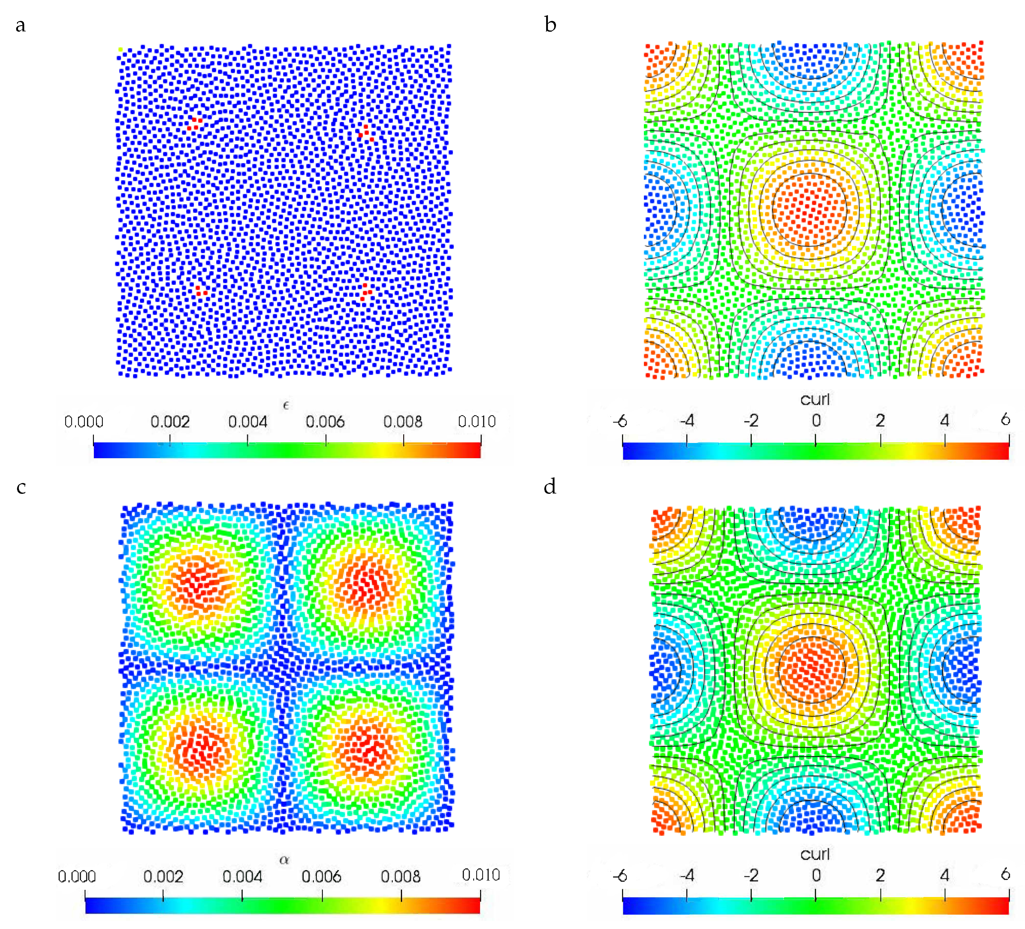
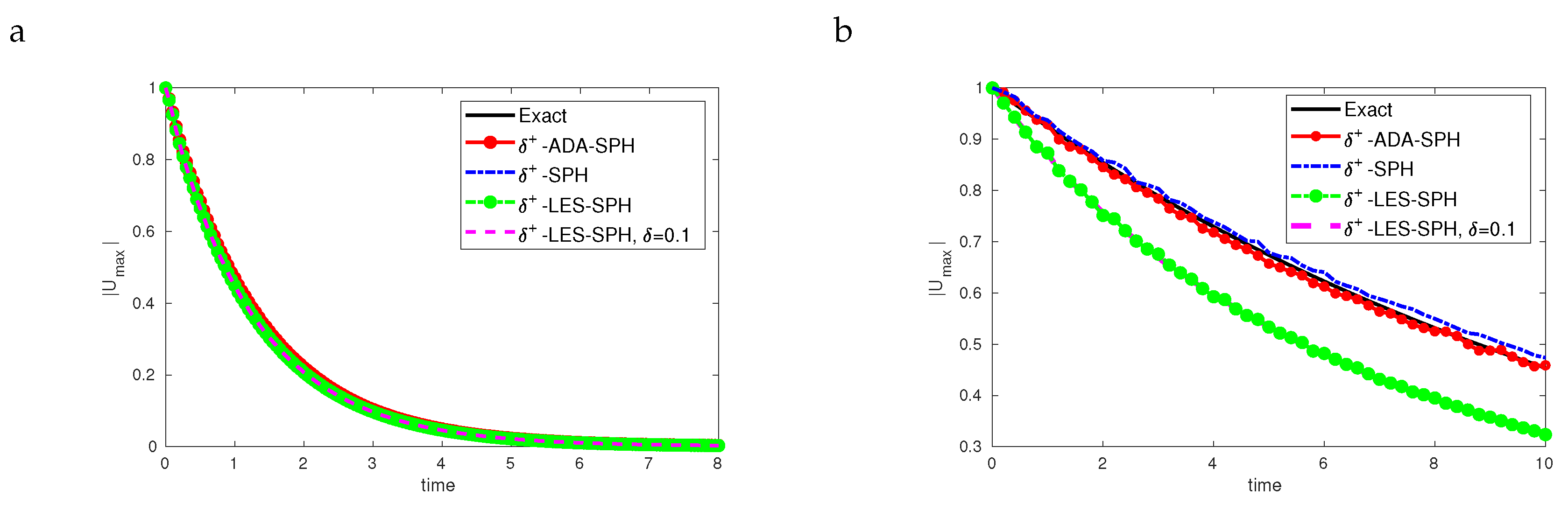
4.1. Viscous Two-Dimensional Taylor–Green Flow

The first test case is the 2D Taylor–Green flow with Reynolds numbers R e = 100 and R e = 1000 . This example is aimed to show that the proposed methodology is able to compute low Mach flows without adding excessive dissipation. The analytic solution of this test case is [36]
u ( x , y , t ) = U e b t cos ( 2 π x ) sin ( 2 π y ) , v ( x , y , t ) = U e b t sin ( 2 π x ) cos ( 2 π y )
where the reference velocity U is set to U = 1 and b = 8 π 2 / R e is the decay rate of velocity field. The density is assumed to be the unity, and the initial pressure is given by
P ( x , y , 0 ) = ρ 0 4 ( cos ( 4 π x ) + cos ( 4 π y ) )
In this test case, the velocity is initiated using t = 0 in Equation (21). This configuration leads to a periodic array of 2 vortices. We use a discretization with 2500 particles. The initial position of the particles is obtained by using the particle packing algorithm described in [37]. We use the value U m a x = 1 for computing Equation (2).
We compare the results using the proposed scheme with those obtained with the original δ + -SPH scheme, the δ -LES-SPH method, and a modified δ -LES-SPH method keeping a constant value of δ = 0.1 . The value of β is set to match the molecular viscosity in the δ -SPH original scheme, and the term related with the added numerical dissipation is neglected ( α i j = 0 ). In δ -LES-SPH and δ -ADA-SPH models, the term ( α i j ) is added to the molecular viscosity, as in Equation (8).
Figure 1 and Figure 2 show the results for the value of the viscous parameters ( ϵ and α ) and the vorticity field at t = 0.5 a for the R e = 100 case and t = 3 for the R e = 1000 case. The vorticity field is in good agreement with the one obtained in [24,38] in the two cases. Concerning the numerical viscosity, it is shown that the proposed methodology introduces a reduced amount of dissipation, compared with the δ -LES-SPH.
The decay of the maximum velocity for the two test cases is plotted in Figure 3 and compared with the theoretical solution [39]. Note that, for the case R e = 1000 , the theoretical solution remains valid until t = 10 [16,29]. The results for the three schemes are practically coincident for the R e = 100 case, and are in agreement with the exact solution. The reason is that the different numerical viscosity introduced by the numerical schemes is not relevant considering the value of the molecular viscosity. The situation changes for R e = 1000 . In this case, the dissipation introduced by the δ -LES-SPH is excessive. It is also seen that for this test case, using a δ parameter constant or variable, marginally affects the results. However, the result obtained of the δ -ADA-SPH method is practically coincident with the theoretical solution [39], since ϵ = 0 in most of the domain, as shown in Figure 2. For this test case, the original δ -SPH scheme lies slightly over the theoretical solution.

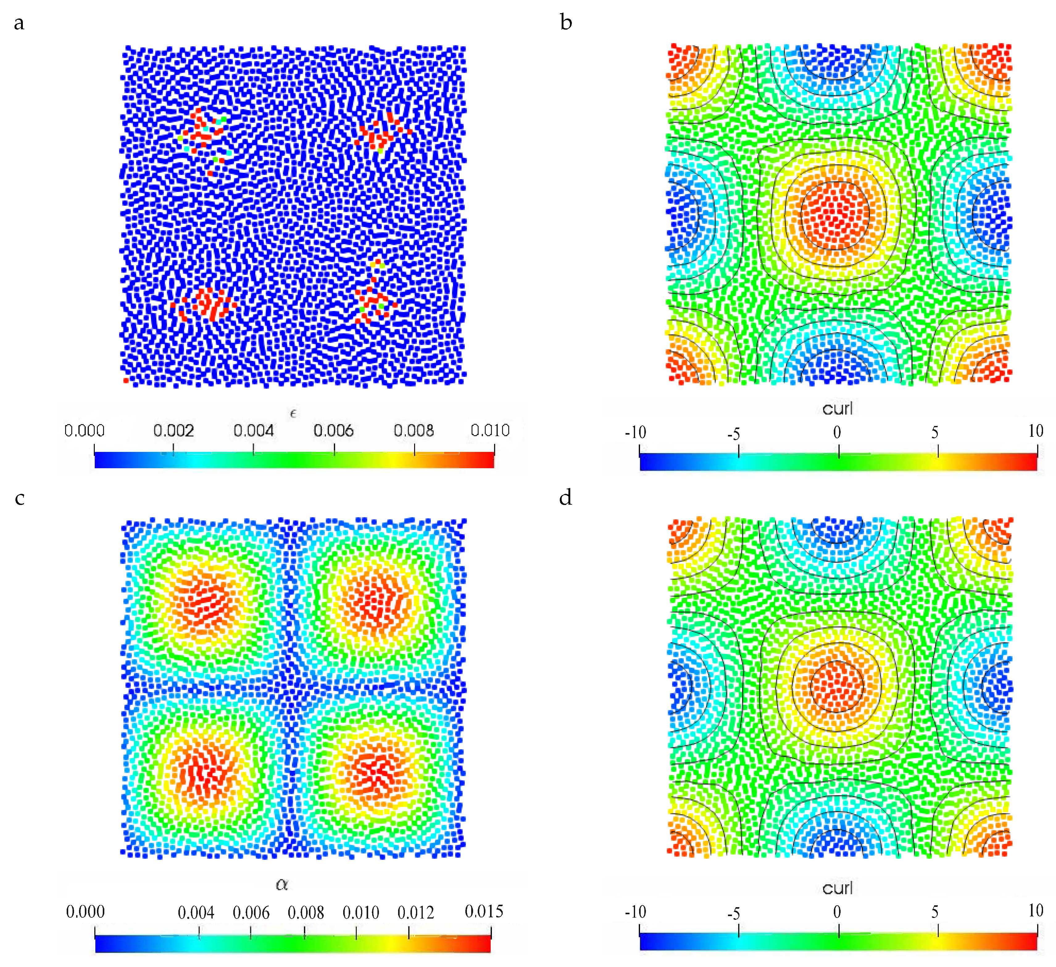
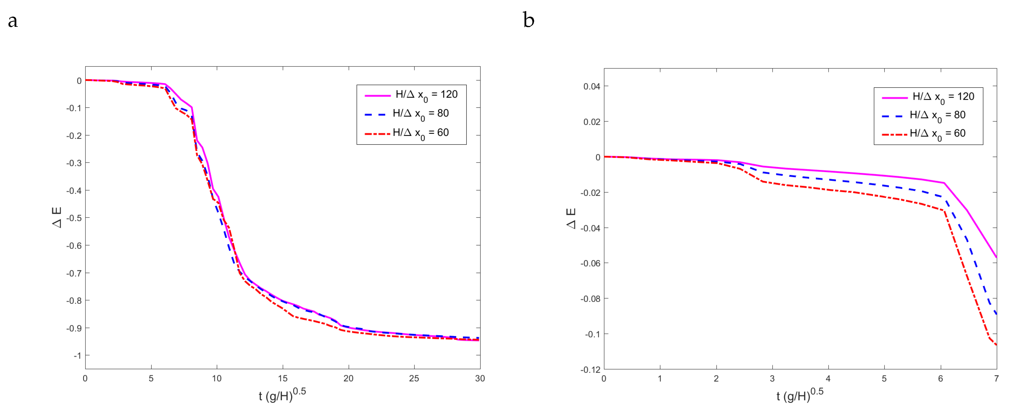
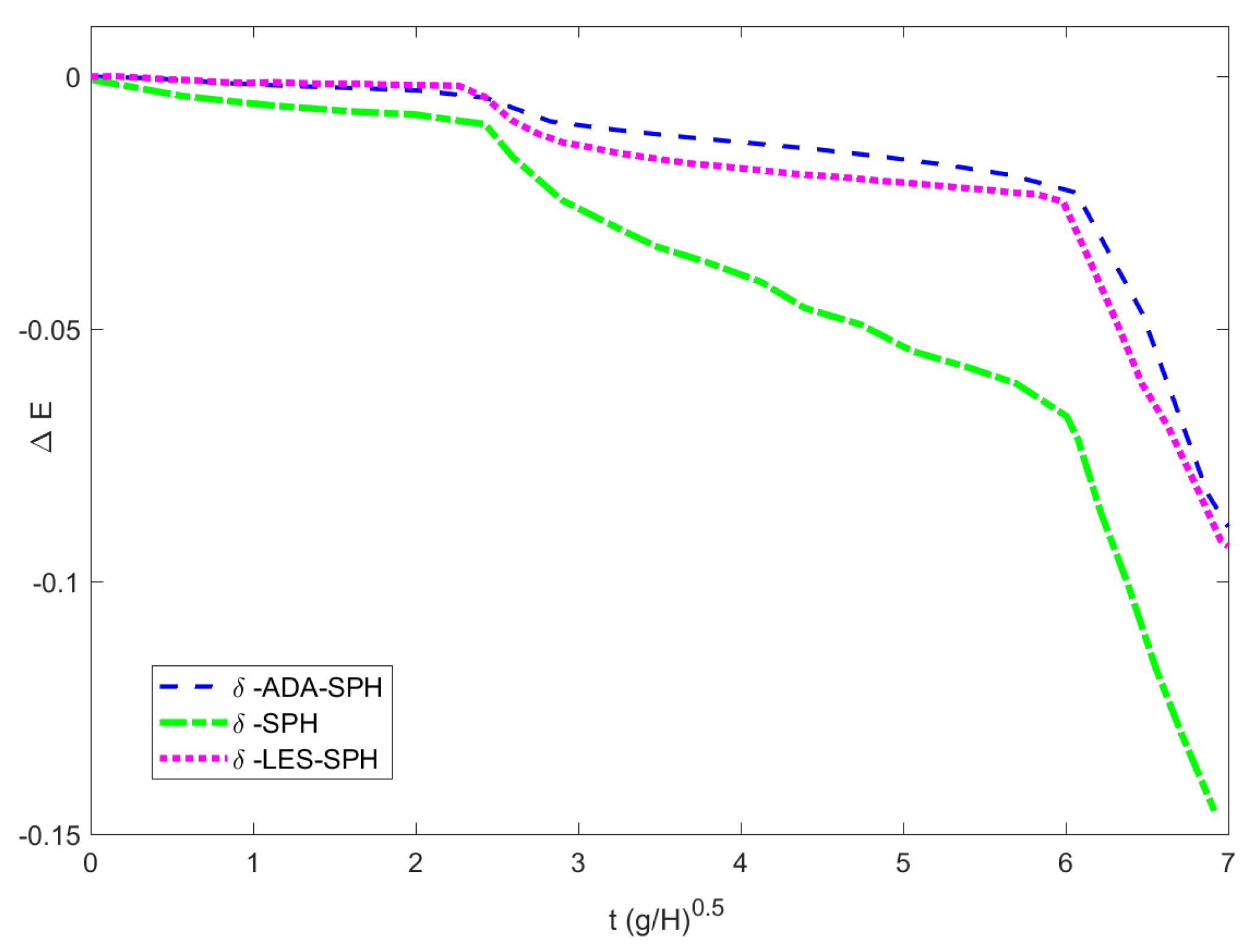
4.2. Inviscid Two-Dimensional Taylor–Green Flow

In this case, we solve the inviscid 2D Taylor–Green vortex. This is equivalent to consider R e = . Thus, the part of β corresponding with the molecular viscosity is set to zero, and the only viscosity introduced in the problem is related to the α parameter, which is adaptive in δ + -ADA-SPH and δ + -LES-SPH methods and constant for the original δ + -SPH. For the latter case, we use a value of α = 0.01 . The use of a constant value of the explicit dissipation is an approach often used for the simulation of inviscid flows with the δ -SPH and δ + -SPH methods [15,25]. Again, we use the value U m a x = 1 for computing Equation (2).
Thus, this test case is intended to determine if the proposed approach is able to recover the physical dynamics in a severely under-resolved simulation. The base case is computed using a resolution of 10,000 particles on a periodic [ 0 , 1 ] × [ 0 , 1 ] square domain. The initial position of the particles is obtained by using the particle packing algorithm described in [37].
In Figure 4, the value of ϵ given by Equation (17) is plotted, together with the resulting vorticity field. It is observed that the scheme is able to capture certain fine structures of the flow. Very interestingly, it is observed that the artificial dissipation is only introduced in regions where the smallest structures of the flow are present. This is specially clear for t = 25 . The core of the final two vortices is well captured by the spatial discretization, and the artificial dissipation is null there. However, out of this region, the resolution is not enough to capture all the fine structures all the flow and the dissipation reaches the maximum value defined. It is also observed that the method is also able to recover the final equilibrium state of two-dimensional decay turbulence, in which a pair of big vortices with opposite sign and with a size comparable to the computational domain appear as a result of merging and pairing of the smaller vortices [24,40,41].
In Figure 5 it is clearly observed that the results obtained for the δ + -LES-SPH and δ + -SPH are clearly over-dissipative. Thus, for this spatial resolution, these methods are not able to recover the fine features of the flow.
This test case is representative of two-dimensional turbulence. Thus, it tests the ability of a new method for simulating this kind of problems. Two-dimensional turbulence has different energy-transfer characteristics than three-dimensional turbulence. Two-dimensional turbulence is characterized by a typical direct entropy cascade with 3 scaling of the energy spectrum [24]. In Figure 6 (left), it is shown that the proposed scheme is able to reproduce the right slope in most of the represented scales, independently of the resolution of the distribution of particles. The slope is not accurate for the highest scales, but this error is quickly reduced as the number of particles is increased. Moreover, in Figure 6 (right), it is shown that the proposed δ + -ADA-SPH scheme, greatly improves the results obtained by other δ + -SPH schemes.
Figure 7 shows the evolution of the kinetic energy. Ideally, it should remain constant and equal to the initial value, since at infinite Reynolds number there is no viscous dissipation. Thus, all the dissipation observed is introduced by the numerical method. When the proposed δ + -ADA-SPH scheme is used, the results are less dissipative than those obtained by the other δ + -SPH schemes. As the grid is refined, the proposed methodology also tends to reduce the dissipation, and, for the resolution of 40,000 particles only a slight decrease of the kinetic energy is observed.
These results can be explained by examination of ϵ and α values. Figure 8 shows the values of these parameters at several times. It is seen that the values of ϵ are consistently lower than those of α , which indicates that the numerical scheme is introducing more dissipation.

5. Lid-Driven Cavity Flow

The lid-driven cavity flow is a classical benchmark widely-studied to test new numerical methods [42,43,44,45,46]. Here, we use this test case to assess the accuracy of the proposed method for wall-bounded flows at different flow regimes. This problem consists of a two-dimensional square cavity filled with an incompressible fluid and covered by four rigid walls of length L. The top wall (lid) moves laterally at a constant velocity U that subsequently creates a fluid motion within the cavity under viscosity effect. The U m a x velocity for Equation (2) is estimated equal to one.
Here, 50 × 50 particles are used to solve the R e = 400 , R e = 1000 and R e = 3200 test cases. The velocity profiles along vertical and horizontal centerlines obtained by the three different schemes are shown in Figure 9 compared with the data of [42].
In general, a good agreement is observed for the three schemes at low Reynolds number. However, as the Reynolds number is increased, the proposed method obtains more accurate results. We also note that, the present 2D simulations obtains a solution that remains steady. Some authors [43] have raised the question about the steadiness and two-dimensionality of this flow at Reynolds numbers higher than 1000.
The analysis of the distribution of the viscous parameters helps to understand these results. Figure 10 shows the values of ϵ and α for the R e = 3200 case. Note that, to facilitate the comparison, we have used the same scale for ϵ and α , but the maximum value achieved by α is more than three times larger than that of ϵ . We notice the large differences in the top boundary and in the top-right corner of the cavity, and the larger dissipation introduced by the δ -LES-SPH around the main vortex.
Figure 11 shows the results obtained using the proposed scheme as the grid is refined. As expected, the numerical solution converges to the reference one and no spurious artifacts are observed.

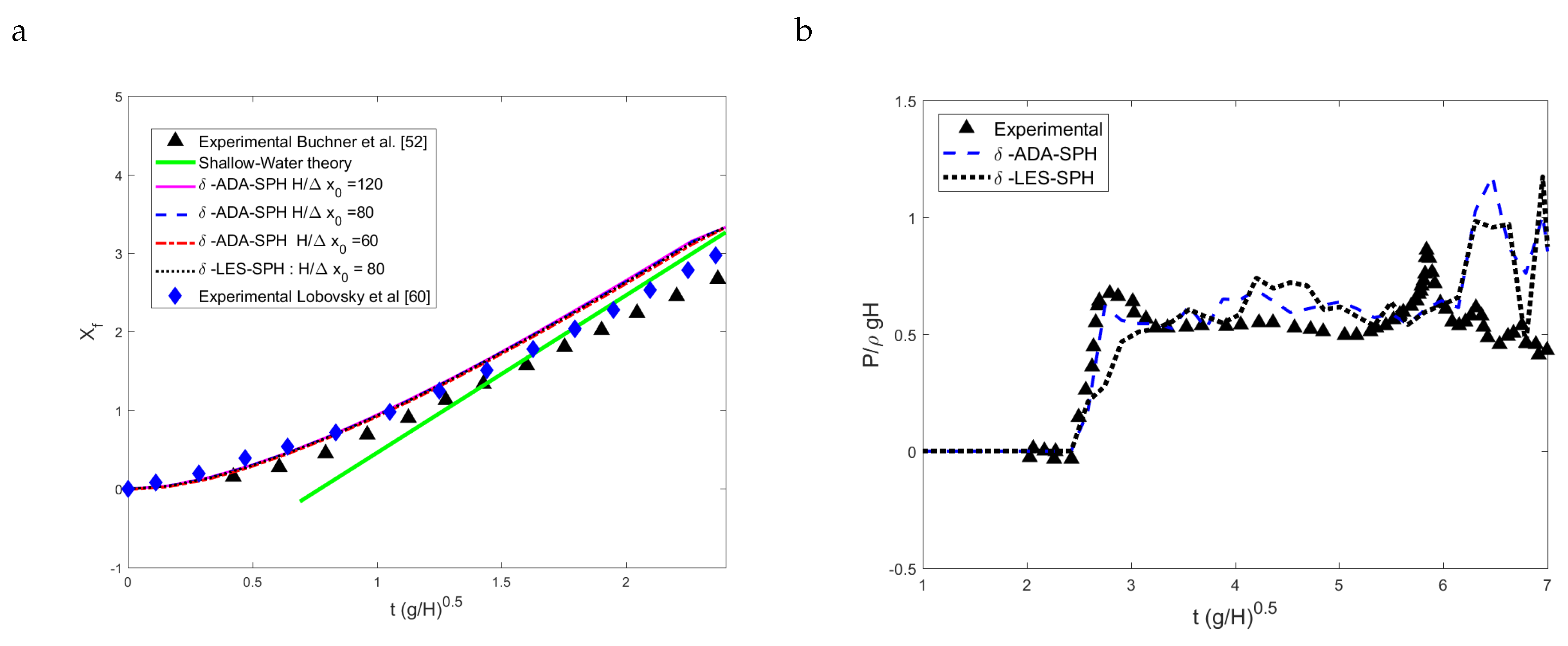
Two-Dimensional Dam-Break Flow

Finally, we consider the two-dimensional dam break problem. The aim of this test case was to assess the ability of the proposed method to deal with complex free-surface flows. This test case has been experimentally investigated by several authors such as Martin et al. [47], Zhou et al. [48] or Buchner [49], among others. This test case addresses a very complex flow with large deformations, and it is one of the most used benchmark to validate SPH and other particle-based methods [25,50,51,52,53]. The initial configuration of the problem is illustrated in Figure 12. A water column of height H and length of 2 H is located in a rectangular tank of length 5.366 H . Here, H is taken equal to 0.6 [m] as in the experimental test of Buchner [49]. Following [13,25], the water flow is considered inviscid with a density value of 1000 [kg/m 3 ], and the effect of gravity is also considered ( g = 0 , 9.81 T ). Thus, the part of β related to the molecular viscosity is set to zero. A pressure probe P located at the downstream wall at y / H = 0.19 , measured from the bottom of the tank (see Figure 12). This position of the probe is slightly different to the one used in the experiments, following the recommendations of [54] to reduce some uncertainties in the measurements.
The generalized wall boundary condition method [50,55] is used to simulate this test case. Three different particle resolutions ( H / Δ x 0 = 120 , 80 , 60 ) are investigated. The pressure field is initialized from the solution of a Poisson equation on the water column [56]. The water column is considered at rest at t = 0 and c 0 = 10 2 g H . The U m a x velocity required for Equation (2) is estimated using Torricelli’s law as in [55].
We note that for this example, the particle shifting technique is not used. As shown in [29], the application of this technique to violent flows causes non-physical behavior, due to accumulation of errors in time. Then the ADA methodology is used combined with the δ -SPH scheme of Marrone et al. [25]. The results obtained are compared with those of the δ -LES-SPH (variable α and δ ) and those of the original δ -SPH scheme [25].
Figure 13 and Figure 14 show snapshots of the evolution of pressure, ϵ and vorticity fields for H / Δ x 0 = 120 . We note that the pressure field is relatively smooth, and no numerical artifacts are detected. Concerning the value of ϵ , it is shown that there are regions with a very small value of this parameter. This indicates a reduction of the numerical viscosity introduced by the numerical method. Moreover, the vorticity field shows the presence of fine scales of the flow.
In order to analyze the water wave front position, we define the adimensional position X f = x f 2 H H , where x f is the x-coordinate of the water front. Figure 15 (left) shows the results obtained by the present methodology for three different particle resolutions, compared with the analytical solution from shallow water theory [57], and the experimental data obtained by Buchner et al. [49] and Lobovskỳ et al. [58]. A good agreement with the theoretical line is obtained with the three discretizations used. A quantitative agreement with the experimental data is also observed, although it should be noted that a slower front wave is observed in the experiments. This could be caused by several factors such as uncertainties of the measurements and wall roughness, as exposed in [59]. Figure 15 (right) shows a comparison of the time evolution of the pressure signals at the probe between the proposed method and the δ -LES-SPH for H / Δ x 0 = 80 . Both numerical models are in quantitative agreement with the experimental data. Note that the different location of the peak of the numerical solutions and experiments, is explained in [51] as the influence of the air-cushioning cavity on the sensor measurement which is not taken into account in the numerical simulation.
In order to study the intrinsic dissipation of the proposed numerical methodology, we analyze the evolution of the mechanical energy ( Δ E ). Here, we use the expression proposed by Marrone et al. [25] to compute Δ E
Δ E = E k i n ( t ) + E p ( t ) E p 0 E p 0 E p
where E k i n ( t ) is the kinetic energy, E p ( t ) the potential energy, E p 0 the initial potential energy and E p the potential energy when the flow reaches a hydrostatic steady state.
Results are plotted in Figure 16. It is observed that the use of the ADA method reduces the differences in the dissipation obtained for different discretizations. This is different to the usual behavior of SPH methods [13,25], and the explanation is that the dissipation is only introduced where the flow is underesolved. Moreover, it is also observed that the flow tends to stabilize and reach the rest state at t g / H = 20 which corresponds well with the experimental results of Buchner [49].
Figure 17 compares the evolution of Δ E before the first splash-up, obtained using the δ -ADA-SPH scheme with the results obtained with the δ -LES-SPH and the results obtained with the original δ -SPH scheme [25], for H / Δ x 0 = 80 . It is clearly observed that for this case, the proposed δ -ADA-SPH scheme outperforms the results of the original δ -SPH scheme and it is slightly less dissipative than the δ -LES-SPH.

6. Conclusions

In this work, an SPH scheme for weakly compressible flows with automatic adaptive numerical dissipation (ADA) is developed. The resulting scheme is a meshless self-adaptive method, in which the introduced artificial dissipation is designed to increase the dissipation in zones where the flow is under-resolved by the numerical scheme, and to decrease it where dissipation is not required. The proposed methodology is applied in the framework of δ -SPH and δ + -SPH formulations. The validation in terms of consistency and accuracy of the presented approach has been studied by means of several two-dimensional benchmarks for different Reynolds numbers: Taylor–Green, lid-driven cavity and dam-break flows. The results show that the proposed numerical method is able to simulate complex flows. It alleviates the parameter dependency of δ -SPH methods and it is generally less dissipative than the δ -LES-SPH model. The obtained results suggest than the proposed approach could be a promising technique for LES computations of transitional flows, where usual SGS models introduce excessive dissipation. This will be the subject of future research.

Author Contributions

Conceptualization, X.N.; methodology, X.N., A.K., L.R., F.N., S.K. and M.D.; software, A.K.; validation, X.N., A.K. and L.R.; formal analysis, X.N., A.K., L.R., F.N., S.K. and M.D.; investigation, X.N., A.K. and L.R.; resources, X.N., A.K., L.R., F.N., S.K. and M.D.; data curation, X.N., A.K., L.R., F.N., S.K. and M.D.; writing—original draft preparation, X.N. and A.K.; writing—review and editing, X.N., A.K., L.R., M.D., S.K. and F.N.; visualization, A.K. and L.R.; supervision, X.N.; project administration, X.N., and L.R.; funding acquisition, X.N., L.R., F.N., S.K. and M.D. All authors have read and agreed to the published version of the manuscript.

Funding

This research was funded by the Ministerio de Ciencia, Innovación y Universidades of the Spanish Government, grant number #RTI2018-093366-B-I00, by the Consellería de Educación e Ordenación Universitaria of the Xunta de Galicia (grant number #ED431C 2018/41). Xesús Nogueira has also been funded by the Xunta de Galicia through the program Axudas para a mellora, creación, reco n ˜ ecemento e estruturación de agrupacións estratéxicas do Sistema universitario de Galicia (grant number # ED431E 2018/11).

Conflicts of Interest

The authors declare no conflict of interest.

References

  1. Gingold, R.A.; Monaghan, J.J. Smoothed particle hydrodynamics: Theory and application to non-spherical stars. Mon. Not. R. Astron. Soc. 1977, 181, 375–389. [Google Scholar] [CrossRef]
  2. Liu, M.; Liu, G. Smoothed particle hydrodynamics (SPH): An overview and recent developments. Arch. Comput. Methods Eng. 2010, 17, 25–76. [Google Scholar] [CrossRef] [Green Version]
  3. Gomez-Gesteira, M.; Rogers, B.D.; Dalrymple, R.A.; Crespo, A.J. State-of-the-art of classical SPH for free-surface flows. J. Hydraul. Res. 2010, 48, 6–27. [Google Scholar] [CrossRef]
  4. Price, D.J. Smoothed particle hydrodynamics and magnetohydrodynamics. J. Comput. Phys. 2012, 231, 759–794. [Google Scholar] [CrossRef] [Green Version]
  5. Violeau, D.; Rogers, B. Smoothed particle hydrodynamics (SPH) for free-surface flows: Past, present and future. J. Hydraul. Res. 2010, 48, 6–279. [Google Scholar] [CrossRef]
  6. Vila, J. On Particle Weighted Methods and Smooth Particle Hydrodynamics. Math. Model. Methods Appl. Sci. 1999, 9, 161–209. [Google Scholar] [CrossRef]
  7. Inutsuka, S.I. Reformulation of smoothed particle hydrodynamics with Riemann solver. J. Comput. Phys. 2002, 179, 238–267. [Google Scholar] [CrossRef] [Green Version]
  8. Sirotkin, F.; Yoh, J. A Smoothed Particle Hydrodynamics method with approximate Riemann solvers for simulation of strong explosions. Comput. Fluids 2013, 88, 418–429. [Google Scholar] [CrossRef]
  9. Avesani, D.; Dumbser, M.; Bellin, A. A new class of Moving-Least-Squares WENO-SPH schemes. J. Comput. Phys. 2014, 270, 278–299. [Google Scholar] [CrossRef]
  10. Hopkins, P. New Class of Accurate, Mesh-Free Hydrodynamic Simulation Methods. Mon. Not. R. Astron. Soc. 2015, 450, 53–110. [Google Scholar] [CrossRef] [Green Version]
  11. Nogueira, X.; Ramírez, L.; Clain, S.; Loubère, R.; Cueto-Felgueroso, L.; Colominas, I. High-accurate SPH method with Multidimensional Optimal Order Detection limiting. Comput. Methods Appl. Mech. Eng. 2016, 310, 134–155. [Google Scholar] [CrossRef] [Green Version]
  12. Ramírez, L.; Nogueira, X.; Khelladi, S.; Krimi, A.; Colominas, I. A very accurate Arbitrary Lagrangian-Eulerian meshless method for Computational Aeroacoustics. Comput. Methods Appl. Mech. Eng. 2018, 342, 116–141. [Google Scholar] [CrossRef] [Green Version]
  13. Zhang, C.; Hu, X.; Adams, N.A. A weakly compressible SPH method based on a low-dissipation Riemann solver. J. Comput. Phys. 2017, 335, 605–620. [Google Scholar] [CrossRef]
  14. Antuono, M.; Colagrossi, A.; Marrone, S.; Molteni, D. Free-surface flows solved by means of SPH schemes with numerical diffusive terms. Comput. Phys. Commun. 2010, 181, 532–549. [Google Scholar] [CrossRef]
  15. Sun, P.; Colagrossi, A.; Marrone, S.; Zhang, A. The δplus-SPH model: Simple procedures for a further improvement of the SPH scheme. Comput. Methods Appl. Mech. Eng. 2017, 315, 25–49. [Google Scholar] [CrossRef]
  16. Di Mascio, A.; Antuono, M.; Colagrossi, A.; Marrone, S. Smoothed particle hydrodynamics method from a large eddy simulation perspective. Phys. Fluids 2017, 29, 035102. [Google Scholar] [CrossRef]
  17. Sun, P.; Colagrossi, A.; Marrone, S.; Antuono, M.; Zhang, A. Multi-resolution Delta-plus-SPH with tensile instability control: Towards high Reynolds number flows. Comput. Phys. Commun. 2018, 224, 63–80. [Google Scholar] [CrossRef]
  18. Meringolo, D.D.; Marrone, S.; Colagrossi, A.; Liu, Y. A dynamic δ-SPH model: How to get rid of diffusive parameter tuning. Comput. Fluids 2019, 179, 334–355. [Google Scholar] [CrossRef]
  19. Li, C.G.; Tsubokura, M. An implicit turbulence model for low-Mach Roe scheme using truncated Navier–Stokes equations. J. Comput. Phys. 2017, 345, 462–474. [Google Scholar] [CrossRef]
  20. Nogueira, X.; Ramírez, L.; Fernández-Fidalgo, J.; Deligant, M.; Khelladi, S.; Chassaing, J.C.; Navarrina, F. An a posteriori-implicit turbulent model with automatic dissipation adjustment for Large Eddy Simulation of compressible flows. Comput. Fluids 2020, 197, 104371. [Google Scholar] [CrossRef]
  21. Tantikul, T.; Domaradzki, J. Large eddy simulations using truncated Navier–Stokes equations with the automatic filtering criterion. J. Turbul. 2010, 11, N21. [Google Scholar] [CrossRef]
  22. Domaradzki, J.A.; Loh, K.C.; Yee, P.P. Large eddy simulations using the subgrid-scale estimation model and truncated Navier–Stokes dynamics. Theor. Comput. Fluid Dyn. 2002, 15, 421–450. [Google Scholar] [CrossRef]
  23. Sun, G.; Domaradzki, J.A. Implicit LES using adaptive filtering. J. Comput. Phys. 2018, 359, 380–408. [Google Scholar] [CrossRef]
  24. Hu, X.; Adams, N. A SPH model for incompressible turbulence. arXiv 2012, arXiv:1204.5097. [Google Scholar] [CrossRef] [Green Version]
  25. Marrone, S.; Antuono, M.; Colagrossi, A.; Colicchio, G.; Le Touzé, D.; Graziani, G. δ-SPH model for simulating violent impact flows. Comput. Methods Appl. Mech. Eng. 2011, 200, 1526–1542. [Google Scholar] [CrossRef]
  26. Liu, M.; Liu, G.; Lam, K. Constructing smoothing functions in smoothed particle hydrodynamics with applications. J. Comput. Appl. Math. 2003, 155, 263–284. [Google Scholar] [CrossRef] [Green Version]
  27. Wendland, H. Piecewise polynomial, positive definite and compactly supported radial functions of minimal degree. Adv. Comput. Math. 1995, 4, 389–396. [Google Scholar] [CrossRef]
  28. Monaghan, J.J. SPH without a tensile instability. J. Comput. Phys. 2000, 159, 290–311. [Google Scholar] [CrossRef]
  29. Sun, P.; Colagrossi, A.; Marrone, S.; Antuono, M.; Zhang, A.M. A consistent approach to particle shifting in the δ-Plus-SPH model. Comput. Methods Appl. Mech. Eng. 2019, 348, 912–934. [Google Scholar] [CrossRef]
  30. Smagorinsky, J. General circulation experiments with the primitive equations: I. The basic experiment. Mon. Weather. Rev. 1963, 91, 99–164. [Google Scholar] [CrossRef]
  31. Deardorff, J.W. A numerical study of three-dimensional turbulent channel flow at large Reynolds numbers. J. Fluid Mech. 1970, 41, 453–480. [Google Scholar] [CrossRef]
  32. Meringolo, D.D.; Liu, Y.; Wang, X.Y.; Colagrossi, A. Energy balance during generation, propagation and absorption of gravity waves through the δ-LES-SPH model. Coast. Eng. 2018, 140, 355–370. [Google Scholar] [CrossRef]
  33. Antuono, M.; Colagrossi, A.; Marrone, S. Numerical diffusive terms in weakly-compressible SPH schemes. Comput. Phys. Commun. 2012, 183, 2570–2580. [Google Scholar] [CrossRef]
  34. Monaghan, J.J. Smoothed particle hydrodynamics. Rep. Prog. Phys. 2005, 68, 1703. [Google Scholar] [CrossRef]
  35. Kennedy, C.A.; Carpenter, M.H.; Lewis, R.M. Low-storage, explicit Runge–Kutta schemes for the compressible Navier–Stokes equations. Appl. Numer. Math. 2000, 35, 177–219. [Google Scholar] [CrossRef] [Green Version]
  36. Taylor, G.I.; Green, A.E. Mechanism of the production of small eddies from large ones. Proc. R. Soc. Lond. Ser. Math. Phys. Sci. 1937, 158, 499–521. [Google Scholar]
  37. Colagrossi, A.; Bouscasse, B.; Antuono, M.; Marrone, S. Particle packing algorithm for SPH schemes. Comput. Phys. Commun. 2012, 183, 1641–1653. [Google Scholar] [CrossRef] [Green Version]
  38. Hu, X.; Adams, N.A. An incompressible multi-phase SPH method. J. Comput. Phys. 2007, 227, 264–278. [Google Scholar] [CrossRef]
  39. Hu, X.; Adams, N.A. A constant-density approach for incompressible multi-phase SPH. J. Comput. Phys. 2009, 228, 2082–2091. [Google Scholar] [CrossRef]
  40. Tabeling, P. Two-dimensional turbulence: A physicist approach. Phys. Rep. 2002, 362, 1–62. [Google Scholar] [CrossRef]
  41. Kraichnan, R.H.; Montgomery, D. Two-dimensional turbulence. Rep. Prog. Phys. 1980, 43, 547. [Google Scholar] [CrossRef]
  42. Ghia, U.; Ghia, K.N.; Shin, C. High-Re solutions for incompressible flow using the Navier-Stokes equations and a multigrid method. J. Comput. Phys. 1982, 48, 387–411. [Google Scholar] [CrossRef]
  43. Erturk, E. Discussions on driven cavity flow. Int. J. Numer. Methods Fluids 2009, 60, 275–294. [Google Scholar] [CrossRef] [Green Version]
  44. Perumal, D.A.; Dass, A.K. Multiplicity of steady solutions in two-dimensional lid-driven cavity flows by lattice Boltzmann method. Comput. Math. Appl. 2011, 61, 3711–3721. [Google Scholar] [CrossRef] [Green Version]
  45. Wahba, E. Steady flow simulations inside a driven cavity up to Reynolds number 35,000. Comput. Fluids 2012, 66, 85–97. [Google Scholar] [CrossRef]
  46. Leroy, A.; Violeau, D.; Ferrand, M.; Kassiotis, C. Unified semi-analytical wall boundary conditions applied to 2-D incompressible SPH. J. Comput. Phys. 2014, 261, 106–129. [Google Scholar] [CrossRef] [Green Version]
  47. Martin, J.C.; Moyce, W.J.; Martin, J.; Moyce, W.; Penney, W.G.; Price, A.; Thornhill, C. Part IV. An experimental study of the collapse of liquid columns on a rigid horizontal plane. Philos. Trans. R. Soc. Lond. Ser. Math. Phys. Sci. 1952, 244, 312–324. [Google Scholar]
  48. Zhou, Z.; De Kat, J.; Buchner, B. A nonlinear 3D approach to simulate green water dynamics on deck. In Proceedings of the Seventh International Conference on Numerical Ship Hydrodynamics, Nantes, France, 19–22 July 1999; pp. 1–15. [Google Scholar]
  49. Buchner, B. Green Water on Ship-Type Offshore Structures. Ph.D. Thesis, Delft University of Technology Delft, Delft, The Netherlands, 2002. [Google Scholar]
  50. Adami, S.; Hu, X.Y.; Adams, N.A. A generalized wall boundary condition for smoothed particle hydrodynamics. J. Comput. Phys. 2012, 231, 7057–7075. [Google Scholar] [CrossRef]
  51. Colagrossi, A.; Landrini, M. Numerical simulation of interfacial flows by smoothed particle hydrodynamics. J. Comput. Phys. 2003, 191, 448–475. [Google Scholar] [CrossRef]
  52. Mokos, A.; Rogers, B.D.; Stansby, P.K.; Domínguez, J.M. Multi-phase SPH modelling of violent hydrodynamics on GPUs. Comput. Phys. Commun. 2015, 196, 304–316. [Google Scholar] [CrossRef]
  53. Chen, Z.; Zong, Z.; Liu, M.; Zou, L.; Li, H.; Shu, C. An SPH model for multiphase flows with complex interfaces and large density differences. J. Comput. Phys. 2015, 283, 169–188. [Google Scholar] [CrossRef]
  54. Greco, M. A Two-Dimensional Study of Green-Water Loading. Ph.D. Thesis, Department of Marine Hydrodynamics, Faculty of Marine Technology, Norwegian University of Science and Technology, Trondheim, Norway, 2001. [Google Scholar]
  55. Krimi, A.; Khelladi, S.; Nogueira, X.; Deligant, M.; Ata, R.; Rezoug, M. Multiphase smoothed particle hydrodynamics approach for modeling soil–water interactions. Adv. Water Resour. 2018, 121, 189–205. [Google Scholar] [CrossRef] [Green Version]
  56. Cherfils, J.M. Développements et Applications de la Méthode SPH aux Écoulements Visqueux à Surface Libre. Ph.D. Thesis, Université du Havre, Le Havre, France, 2011. [Google Scholar]
  57. Ritter, A. Die fortpflanzung der wasserwellen. Z. Des Vereines Dtsch. Ing. 1892, 36, 947–954. [Google Scholar]
  58. Lobovskỳ, L.; Botia-Vera, E.; Castellana, F.; Mas-Soler, J.; Souto-Iglesias, A. Experimental investigation of dynamic pressure loads during dam break. J. Fluids Struct. 2014, 48, 407–434. [Google Scholar] [CrossRef] [Green Version]
  59. Rezavand, M.; Zhang, C.; Hu, X. A weakly compressible SPH method for violent multi-phase flows with high density ratio. J. Comput. Phys. 2020, 402, 109092. [Google Scholar] [CrossRef] [Green Version]
Figure 1. Two-dimensional Taylor–Green flow at R e = 100 . On the top the viscosity parameter ( ϵ ) (a) and the vorticity field (b) obtained with the proposed δ -ADA-SPH scheme. On the bottom we show the value of the α parameter (c) and the vorticity field (d) using the δ -LES-SPH scheme. Results obtained at t = 0.5 .
Water 12 02858 g001
Figure 2. Two-dimensional Taylor–Green flow at R e = 1000 . On the top, the viscosity parameter ( ϵ ) (a) and the vorticity field (b) obtained with the proposed δ -ADA-SPH scheme. On the bottom we show the value of the α parameter (c) and the vorticity field (d) using the δ -LES-SPH. Results obtained at t = 3 .
Water 12 02858 g002
Figure 3. Two-dimensional Taylor–Green flow. Decay of the maximum velocity for R e = 100 (a) and R e = 1000 (b). The theoretical solution is taken from [39].
Water 12 02858 g003
Figure 4. Inviscid two-dimensional Taylor–Green flow. On the left, value of ϵ given by Equation (17). On the right, vorticity field. Figures (a,c) show the results at t = 2 and figures (b,d) show the results obtained at t = 25 , using a resolution of 10,000 particles.
Water 12 02858 g004
Figure 5. Inviscid two-dimensional Taylor–Green flow. Vorticity field for t = 2 . Figure (a) shows the results using the δ + -SPH scheme with a constant value of α = 0.01 . Figure (b) shows the results obtained using the δ + -LES-SPH approach. Results computed using a resolution of 10,000 particles.
Water 12 02858 g005
Figure 6. Inviscid two-dimensional Taylor–Green flow. Figure (a): Energy spectrum obtained using the proposed δ + -ADA-SPH method with different particle resolutions. Figure (b): comparison of the results using different δ + -SPH schemes using a resolution of 10,000 particles (right).
Water 12 02858 g006
Figure 7. Inviscid two-dimensional Taylor–Green flow. Evolution of the kinetic energy using different schemes and different particle resolutions.
Water 12 02858 g007
Figure 8. Inviscid two-dimensional Taylor–Green flow. Results for ϵ and α fields. On the left, the results obtained using the δ + -ADA-SPH for t = 0.5 (a), t = 2 (c) and t = 20 (e). On the right, the results obtained using the δ + -LES-SPH [16] approach for t = 0.5 (b), t = 2 (d) and t = 20 (f). Results computed using a resolution of 10,000 particles.
Water 12 02858 g008aWater 12 02858 g008b
Figure 9. Lid-driven cavity flow: Velocity profiles along vertical (left) and horizontal (right) centerlines, computed for three different Reynolds numbers using 50 × 50 particles. The normalized u-velocity component is plotted on the left, whereas the normalized u-velocity component is plotted on the right. The solutions are compared with those of Ghia [42]. Figures (a,b) show the results for R e = 400 , figures (c,d) plot the results for R e = 1000 and figures (e,f) show the results obtained for R e = 3200 .
Water 12 02858 g009
Figure 10. Lid-driven cavity flow: Results for ϵ and α fields for R e = 3200 . Figure (a): Results obtained using the δ + -ADA-SPH are plotted. Figure (b): Results obtained using the δ + -LES-SPH [16] approach. Results computed using a resolution of 50 × 50 particles.
Water 12 02858 g010
Figure 11. Lid-driven cavity flow: Normalized velocity profiles along vertical (a) and horizontal (b) centerlines, computed for Reynolds number R e = 3200 using 50 × 50 , 100 × 100 and 200 × 200 particles. The solutions are compared with those of Ghia [42].
Water 12 02858 g011
Figure 12. Two-dimensional dam-break flow: problem configuration.
Water 12 02858 g012
Figure 13. Two-dimensional dam-break flow: Snapshots of the computational results at different times t g / H for H / Δ x 0 = 120 . On the left column the pressure field is presented, ϵ field is placed on the right. Figures (a,b) shows the results for t g / H = 2.35 , (c,d) shows the results at t g / H = 4.04 , whereas (e,f) plots the results for t g / H = 7.12 . Figures (g,h) shows the results obtained at t g / H = 7.12 .
Water 12 02858 g013aWater 12 02858 g013b
Figure 14. Two-dimensional dam-break flow: Snapshots of the computational results for different times t g / H with H / Δ x 0 = 120 . On the left column the vorticity field is presented, ϵ field is placed on the right. Figures (a,b) show the results for t g / H = 9.54 , (c,d) show the results at t g / H = 13.02 , figures (e,f) plots the results for t g / H = 19.09 and (g,h) shows the results obtained at t g / H = 21.033 .
Water 12 02858 g014aWater 12 02858 g014b
Figure 15. Two-dimensional dam-break flow. Figure (a) shows the time evolution of the water front. The green solid line shows the analytical solution from shallow water theory [57] and the black triangles shows the experimental data given by Buchner [49]. The blue diamond shows the experimental data given by Lobovskỳ et al. [58]. Magenta (solid), blue (dashed) and red (dash-dot) lines shows the results obtained by the proposed scheme with H / Δ x 0 = 120 , 80 and 60, respectively. Figure (b) shows the time evolution of the pressure signals recorded at P is presented. The blue dashed line presents the results obtained by using the presented δ -ADA-SPH model. The magenta dotted line presents the results obtained with δ -LES-SPH approach. The particle resolution is H / Δ x 0 = 80 .
Water 12 02858 g015
Figure 16. Two-dimensional dam-break flow. Figure (a) shows the time evolution of mechanical energy. Figure (b) plots the results obtained by the proposed method with different particle resolution. A zoom of the region of the curve before the first splash-up is displayed on the right.
Water 12 02858 g016
Figure 17. Two-dimensional dam-break flow: Time evolution of mechanical energy. The blue dashed line shows the results obtained by the present δ -ADA-SPH scheme. The magenta dotted line presents the results obtained with the δ -LES-SPH approach. Finally, the green dash-dot line presents the results obtained in [25] using δ -SPH scheme. All the results are computed with H / Δ x 0 = 80 .
Water 12 02858 g017
Publisher’s Note: MDPI stays neutral with regard to jurisdictional claims in published maps and institutional affiliations.

