Large Eddy Simulation of Near-Bed Flow and Turbulence over Roughness Elements in the Shallow Open-Channel

Abstract

Turbulent flows in rough open-channels have complex structures near the channel-bed. The near-bed flow can cause bed erosion, channel instability, and damages to fish habitats. This paper aims to improve our understanding of the structures. Transverse square bars placed at the channel-bed form two-dimensional roughness elements. Turbulent flows over the bars are predicted using large eddy simulation (LES). The predicted flow quantities compare well with experimental data. The LES model predicts mean-flow velocity profiles that resemble those in the classic turbulent boundary layer over a flat plate and profiles that change patterns in the vicinity of roughness elements, depending on the pitch-to-roughness height ratio $\lambda /k$. The relative turbulence intensity and normalized Reynolds shear stress reach maxima of 15% and 1.2%, respectively, at $\lambda /k$ = 8, compared to 9% and 0.2% at $\lambda /k$ = 2. The predicted bottom boundary layers constitute a large portion of the total depth, indicating roughness effect on the flow throughout the water column. Fluid exchange between the roughness cavity and outer region occurs due to turbulence fluctuations. The fluctuations increase in intensity with increasing $\lambda /k$ ratio. This ratio dictates the number of eddies in the cavity as well as their locations and shapes. It also controls turbulence stress distributions. LES can be used to explore strategies for erosion control, channel restoration, and habitat protection.

1. Introduction

Turbulent flows of water or air as a viscous fluid, bounded by a rigid boundary, are an important class of basic flows [1]. There is an abundance of examples of such flows, including water flow along a river channel-bed, air flow around a rigid body, and pressure flow of a liquid between two parallel planes. A common feature of these flows is that there exists an equilibrium layer of wall turbulence near the boundary. The channel-bed as a rigid boundary directly influences the structure of wall turbulence, and the viscosity of water transmits the influence upward across the water column [2]. The strength of the near-bed flow and turbulence have important implications. They can cause significant channel-bed erosion, sediment scour around the foundations of in-stream hydraulic infrastructures (e.g., bridge piers), and damages to fish habitats. They can increase hydrodynamic forces on pipelines placed across river channels, and hence affect adversely their stability. Clearly, the study of near-bed flow and turbulence is of engineering relevance and practical importance.

Previously, a great deal of research attention has been paid to the classic problem of turbulent boundary layer along a flat plate, leading to an impressive progress [3,4,5]. This includes empirically-determined relationships for the mean streamwise velocity, $U_1$, and shear stress, $\tau$, as well as details about turbulence intensity, shear stress, kinetic energy, eddy viscosity, and dissipation (e.g., [6,7]). The law of the wall is one of the key relationships, stating that u can be correlated in terms of the shear stress at the surface, ${\tau }_o$, the distance from the surface, y, and fluid properties (density $\rho$ and molecular viscosity $\nu$). The fluid in contact with the plate surface has zero velocity, and $U_1$ rapidly increases with y from zero to the freestream value, $U_e$, across the boundary-layer thickness, $\delta$.

The thickness $\delta$ divides into three distinct sub-regions: a viscous sublayer, an inertial sublayer, and a defect layer. The viscous sublayer extends from the surface to the wall distance $y^{+}=5$, with a thickness of the order of ${10}^{-3}\delta$ to ${10}^{-2}\delta$ [6] and a linear velocity distribution. The velocity is unsteady, but due to the overwhelming effects of the viscosity, the Reynolds stress associated with velocity fluctuations does not contribute much to the total stress. The inertial sublayer typically lies between $y^{+}=30$ and $0.1\delta$ [8]. The value of $y^{+}$ at the upper boundary depends on the Reynolds number, reportedly being $y^{+}=500$. The velocity distribution is logarithmic. A buffer layer exists as a merge zone between the logarithmic velocity distribution and the viscous sublayer. The defect layer lies between the logarithmic layer and the edge of the boundary layer (above $y^{+}=500$). This layer is a large fraction of the total boundary-layer thickness. The velocity distribution close to the wall is directly related to the kind and magnitude of the wall roughness [6] (p. 484). For flow over a rough wall, the law of the wall is given by $u^{+}={\kappa }^{-1}ln(y/k)+8.5$, where k is the roughness height.

The knowledge of turbulent boundary layer summarized above is based on an abundant amount of experimental data available. The data are mostly from experiments of flows along a flat plate. In comparison, there is very limited data available about flows along a rigid surface with roughness elements. The rough surfaces create near-boundary flows with much complex eddy structures that cannot adequately be represented by the established laws of velocity and turbulence distributions. Rau et al. [9] provided experimental evidence that the flow in a rib-roughened square duct was highly three-dimensional, with strong secondary motions. They remarked that simple correlations based on the law of the wall and the Reynolds analogy were invalid to describe the observed flow field.

Perry et al. [10] introduced the terms k-type of roughness and d-type of roughness in an investigation of pipe flow (k is roughness scale and d pipe diameter). Note that $k/d$ represents the relative scale of roughness. Regarding the k-type of roughness, at sufficiently high values of the Reynolds number, $Re$, the pipe flow becomes independent of viscosity and is a function of $k/d$ alone. The d-type of roughness features closely spaced elements (a smooth wall surface with a series of depressions or cavities); the outer flow generates stable vortices in the cavities, and eddy shedding from the elements into the outer region is negligible. Chow [11] (p. 197) discussed the concept of roughness in the context of open-channel flow. The rough surface flow in open channels was classified into three basic types: isolated-roughness flow, wake-interference flow, and quasi-smooth flow, based on the ratio $\lambda /k$, where $\lambda$ is the longitudinal spacing of the roughness elements. The discussion was qualitative and was limited to the case of two-dimensional roughness elements. In open channels, roughness elements are typically a three-dimensional object. Townsend [1] (p. 139) used the roughness Reynolds number ($R_r=u_{*}k/\nu$) in discussion of rough surface flow. The focus is on the mean-velocity distribution rather than the flow around roughness elements or eddy structures.

Some researchers measured turbulent flows around roughness elements, with emphases on different aspects of the rough surface flow problem. For example, Bagherimiyab and Lemmin [12] obtained acoustic Doppler velocity profiler measurements of the friction velocity $u_{*}$. They reported up to 20% differences of $u_{*}$ estimates using various analytical formulations from the measured values. Tachie and Adane [13] made particle image velocimetry measurements of velocity and turbulence distributions for flows over the k-type and d-type of roughness for a few values of the ratio $\lambda /k$. Djenidi et al. [14] made laser Doppler velocimetry measurements of the flow structure in two-dimensional square cavities. They showed significant exchange of fluid mass between the outer flow region and the cavities. They remarked the association of the exchange with the passage of near-wall quasi-streamwise vortices. They observed a local maximum in the Reynolds shear stress in the shear layers over the cavities. Mass exchange was also observed in Volino et al. [15]. Okamoto et al. [16] measured turbulence intensities of flow over two-dimensional square bars at $\lambda /k=2,5,$ and 9, and concluded that the roughness at $\lambda /k=9$ produced the maximum augmentation of turbulence intensities.

Hinze [6] stated that there is great variety in the possibilities of wall turbulence, depending on the nature and configuration of the boundary. The bounding beds of turbulent open-channel flows are typically rough boundaries. Boundary layers form near the beds and their nature dictates many properties of the flows. In practice, the beds can have a wide range of geometric configurations such as various bedforms, ridges, or other irregular geometric features over the bed surfaces. Thus, it is not economically feasible to conduct laboratory experiments to cover an extensive range of boundary configurations and flow conditions.

Large eddy simulation (LES) [17,18] is an advanced computational technique for numerical solutions to the Navier–Stokes equations. The technique is suitable to deal with flows of a wide range of time and length scales in complex geometry. LES filters out motions of the smallest length scales from the numerical solution but retains their effect on the resolved flow field. For near-wall flows, LES has the potential to capture much more detailed flow structures than computational models based on the Reynolds-averaged Navier–Stokes equations. On the other hand, LES incurs lower computing costs than direct numerical simulation, which intends to resolve all the motions down to the Kolmogorov microscales (or the smallest scales in turbulent flow). This paper demonstrates the effectiveness of LES by comparing numerical predictions with available measurements of flow variables from laboratory experiments of turbulent flow over surface roughness [13]. With a rapidly growing computing power, LES may be applied to simulate the detailed structures of high Reynolds number flows in increasingly large domains. In most cases, existing LES models have assumed a fully developed boundary layer under zero-pressure gradient. This assumption may be acceptable for rough surface flow in deep channels, but it is questionable for flow in shallow channels. In the latter case, the boundary-layer thickness is a significant fraction of the total flow depth [13]. Some researchers computed rough surface flow using direct numerical simulation (DNS) [19,20,21]. DNS suffers the limitation of low Reynolds numbers and hence uncertain scale effects.

This paper aims to improve our understanding of near-bed flow structures and turbulence characteristics by means of LES. LES was performed using Ansys Fluent [22]. LES results of turbulent flow over two-dimensional roughness elements in shallow open channels are presented, along with validation of the results using the experimental data of Tachie and Adane [13]. The main novelty of this paper lies in detailed quantification of complex eddy motions and turbulence distributions around the roughness elements. It is found that the ratio $\lambda /k$ dictates the number of eddies in the cavity as well as their locations and shapes. With the k-type of roughness, the mean-velocity profiles change patterns, and turbulence fluctuations have stronger intensities, compared to those with the d-type of roughness. The experimental and numerical results play complementary roles. The former was essential for checking the accuracy of the latter, whereas the latter extended the former in two aspects. One aspect was that the latter covered more $\lambda /k$ conditions than the former. The other aspect was that the latter produced more details of near-bed flow. It is understood that the former intrinsically captured three-dimensionality, whereas the latter was limited to two dimensions. The numerical modeling strategies reported in this paper would be beneficial to modeling studies of riverbed sediment suspension and transport, channel erosion, and water turbidity control, safety protection of in-stream hydraulic infrastructures, and restoration of healthy fish habitats.

2. Methods

2.1. The Continuity and Navier–Stokes Equations

For an incompressible viscous fluid, the continuity and Navier–Stokes equations in three dimensions govern the fluid motion. The fluid motion over roughness elements at the channel-bed comprises eddies of a wide range of scales. For numerical solutions to the governing equations, LES filters out eddies of length scales smaller than the employed mesh size (filter width $\mathsf{\Delta }$) or subgrid-scale motion for short, and computes larger eddies which carry most of the flow energy and cause most of turbulent mixing of momentum. The filtering operations separate small-scale eddies from large-scale eddies. The effect of the small-scale eddies is modeled using a subgrid-scale scheme. Some popular filters are: the simple volume-average box filter, the Fourier cutoff filter, and Gaussian filter. In this paper, the finite volume discretization of the governing partial differential equations itself implicitly provides filtering operations, and converts them to filtered continuity and Navier–Stokes equations

$$\frac{\partial u_j}{\partial x_j}=0$$

(1)

$$\frac{\partial u_i}{\partial t}+\frac{\partial \left(u_i{u}_j\right)}{\partial x_j}=-\frac{1}{\rho }\frac{\partial P}{\partial x_i}+\frac{\partial }{\partial x_j}(\nu \frac{\partial u_i}{\partial x_j}+{\tau }_{ij})$$

(2)

where $u_i$ is the $x_i$ component of the resolvable-scale filtered velocity ($i=1,2,3$); t is the time; P contains the resolved-scale filtered pressure; ${\tau }_{ij}$ is the subgrid-scale stresses. The stresses include the Leonard stress, the cross-term stress, and the subgrid-scale Reynolds stress. They are associated with the interaction of fluctuations of larger-scale resolvable fields, the interaction of resolvable and unresolvable fluctuations, and the interaction of unresolvable fluctuations, respectively. Some of the popular eddy viscosity models for computation of ${\tau }_{ij}$ are the purely algebraic Smagorinsky model, its dynamic variant, and the wall-adapted local eddy-viscosity model [23]. More details about the LES formulations can be found in Wilcox [8].

2.2. Subgrid-Scale Turbulence Model

For LES of rough surface flow, Dritselis [24] compared the performance of three subgrid-scale turbulence models: the standard dynamic Smagorinsky model [25], the Lagrangian dynamic Smagorinsky model [26], and the coherent structure model [27]. The comparison confirmed the suitability of the standard dynamic Samagorinsky model. This model is used in the present study for computation of ${\tau }_{ij}$. This model splits the stresses into an isotropic and an anisotropic component. The isotropic component is twice the kinetic energy of the subgrid-scale fluctuations, and is included in P in Equation (2) [8] (p. 439). The anisotropic component is related to the resolved strain rate, $S_{ij}$, through an eddy viscosity. Details of the dynamic subgrid-scale model can be found in Germano et al. [25].

2.3. Geometry Description

Four production runs of LES were performed in this study. Two-dimensional rough surfaces were created by placing transverse square bars at the bed of an open channel (Figure 1).

Table 1. Model channel dimensions, roughness characteristics, mesh, and hydraulic conditions for LES runs.

Run	D	L	k	$\mathit{\lambda }/\mathit{k}$	N	$\mathsf{\Delta }\mathit{t}$	f	${\mathit{U}}_{\mathit{e}}$	T	Re	Fr
	(m)	(m)	(m)			(s)	(Hz)	(m/s)	(s)
1	0.075	0.156	0.006	2	1,117,857	0.001	20	0.400	0.39	27,600	0.49
2	0.075	0.168	0.006	4	769,674	0.0001	10	0.395	0.43	27,255	0.48
3	0.075	0.18	0.006	6	640,100	0.0001	10	0.386	0.47	26,634	0.47
4	0.075	0.48	0.006	8	1,689,732	0.001	10	0.380	1.26	26,220	0.46

lists the roughness, mesh, and hydraulic conditions for the four runs. In the table, D is the flow depth (from the water surface to the channel-bed), L is the channel length, N is the total number of computing nodes, $\mathsf{\Delta }t$ is the time step, f is the frequency of LES output sampling, $U_e$ is the freestream velocity, T is the advection time scale (or the time scale for fluid particles to flow through the channel length), Re is the Reynolds number (Re = $U_{e}H/\nu$, where $H=D-k$), and Fr is the Froude number (Fr = $U_e/\sqrt{gH}$, where g is the gravitational acceleration). The flows were turbulent (with Re $>2.0\times {10}^5$) and subcritical (with Fr $<1$). The time step was chosen to achieve numerical stability and accuracy. Among the runs, Run 4 had the largest $\lambda /k$ ratio, which was expected to produce the most complex turbulence structures. For the conditions of Runs 1 and 4, experimental data [13] are available for comparison.

In Figure 1, the model channels for Runs 1 to 4 had a length (in the $x_1$-direction) of 0.156, 0.168, 0.18, and 0.48 m, respectively. The square bars were evenly placed at the channel-bed. Their dimensions are 0.006, 0.006, and 0.075 m in the $x_1$-, $x_2$-, and $x_3$-direction, respectively. The channel length was more than two times the flow depth, giving a balance between computing costs and computational accuracy. A certain length may work in favor of a corresponding wave frequency. The preference was to use the largest length possible to allow flow development, within the capacity of available computing resources. The strategy used in this paper was to minimize the possible domination of a certain wave number and include the realistic category of different wave numbers.

2.4. Boundary Conditions

The model channel (Figure 1) had five types of boundaries: (1) inlet (at $x_1=0$); (2) outlet (at $x_1=L$); (3) lateral boundaries (at $x_3=0$ and $x_3=0.075$ m); (4) water surface (at $x_2=H$); and (5) channel-bed (at $x_2=-k$).

• Cyclic condition was applied in the $x_1$-direction between the inlet and outlet.
• Similarly, cyclic condition was applied in the $x_3$-direction between the two lateral boundaries.
• The water surface was approximated as a rigid lid, on which the shear stresses in the $x_1$- and $x_3$-direction were zero and the normal velocity was zero (or $u_2=0$).
• The channel-bed was a no-slip wall, at which all velocity components were zero (or $u_i=0$).

The use of cyclic conditions reduces computing costs. Two pairs of periodic-shadow zones were created for circulating flow in the $x_1$- and the $x_3$-direction, respectively. The velocity components at the outlet translated horizontally back to the inlet. Similarly, the velocity components on one of the lateral boundaries translated horizontally back to the other lateral boundary. The mass flow rates were specified for the applications of the periodic boundary conditions. The mass flow rates were 1.8138, 1.7138, 1.7138, and 1.517 kg/s for Runs 1 to 4, respectively. These specified flow rates produced values of the freestream velocity, $U_e$, very close to those in the experiments of Tachie and Adane [13].

2.5. Grid Configuration

The model-channel dimensions, geometric complexity and mesh resolutions, $\mathsf{\Delta }{x}_i$ ($i=1,2,3$), determine the total number of computing nodes and hence computing costs. The mesh was generated using Ansys Integrated Computer-aided Engineering and Manufacturing software. Near-wall regions were covered with fine mesh through local refinements in order to accurately resolve flow details. The fine mesh resolved the viscous sublayer. The first node immediately off a wall (e.g., the channel-bed, and bar surfaces) had a wall distance $y^{+}$≈ 1. The growth rate of mesh sizes was lower than 1.2. Mesh-independence tests were carried to determine the required mesh resolutions, following some recommendations given in Choi and Moin [28] and Gerasimov [29]. An example of mesh configurations is shown in Figure 2. A summary of mesh resolutions is given in

Table 2. Mesh sizes and size growth-rates for the outer region and cavity. In a pair of parentheses, the values are the range of $\mathsf{\Delta }{x}_1$, followed by the range of $\mathsf{\Delta }{x}_2$, both in dimensionless wall units. The positions of the roughness-top surface, cavity-bed and water surface are marked in Figure 1.

Run	Mesh Size			Growth Rate
	Roughness-Top Surface	Cavity-Bed	Water Surface	Cavity	Outer Region
1	(4.8–19.3, 1–9.7)	(9.7–19.3, 1–9.7)	(9.7–38.6, 48.3)	1.2	1.05
2	(4.8–19.3, 1–9.7)	(9.7–28.9, 1–9.7)	(9.7–38.6, 48.3)	1.1	1.05
3	(4.8–19.3, 1–9.7)	(9.7–38.6, 1–9.7)	(9.7–38.6, 48.3)	1.1	1.05
4	(4.8–19.3, 1–9.7)	(9.7–38.6, 1–9.7)	(9.7–38.6, 67.5)	1.2	1.05

.

For the hydraulic conditions given in Table 1, a wall distance $y^{+}=1$ corresponds to about 0.05 mm. In the $x_3$-direction, for Runs 1 and 4, the mesh size was 1.5 mm; for Runs 2 and 3, the mesh sizes were 0.8 mm in the center region and 4 mm near the lateral boundaries. In addition to the runs listed in Table 2, some test runs, which used the same conditions as Run 4 but finer mesh resolutions, were carried out to confirm the independence of LES results on mesh configurations.

3. Results

3.1. Mean Flow Velocity

Each of the model runs (Table 1) commenced from an initial state of rest and lasted a model time period much larger than the advection time scale, T. T was determined from the channel length, L, and the free stream velocity, $U_e$, as $T=L/U_e$. For each run, after 10T (a spin-up time period for the flow to develop from the initial state of rest), data were sampled from LES outputs for further analysis. The spin-up time of 10T ensured that the artificial influence of the initial condition had diminished before data sampling. The LES outputs were sampled at a frequency $f=10$ or 20 Hz (Table 1) over a time period of 6 s. For each run, the sampling provides 60 or 120 snapshots of turbulent flow field ($n=60$ or 120), which is large enough to allow a statistically valid analysis. For a given node, the mean flow velocity component, $U_i$, in the $x_i$-direction ($i=1,2,3)$ was obtained by taking the arithmetic mean of the n snapshot values of $u_i$

$$U_i=\frac{1}{n}\sum _1^n{u}_i$$

(3)

For Run 1 (Table 1), the model channel had a total of 13 transverse square bars over the channel length (between $x_1=0$ m at upstream and $x_1=L=0.156$ m at downstream). Vertical profiles of $U_1$ (Equation (3)) at nine selected $x_1$ locations between the 7th and 8th bars are plotted as curves in Figure 3. The locations between adjacent profiles were approximately one-eighth of $\lambda$ apart. Note that the top surfaces of the two bars were at $x_2/k=0$ between $x_1/\lambda =6.25$ and 6.75, and at $x_2/k=0$ between $x_1/\lambda =7.25$ and 7.75, respectively; the cavity bed between the two bars was at $x_2/k=-1$ between $x_1/\lambda =6.75$ and 7.25 (Figure 1). In the vertical direction, the lowest data points of profiles 1 to 3 and 7 to 9 were at the bar top surface, having zero values of $U_1$ and non-zero values of $x_1/\lambda$ (indicating the $x_1$ locations of the profiles). Similarly, the lowest data points of profiles 4 to 6 were at the cavity bed, with $U_1=0$, and $x_1/\lambda >0$ (the profiles’ longitudinal locations). The highest data points of all the profiles were at the water surface (at $x_2/k=11.5$). Profiles 1 and 9 corresponded to each other in terms of longitudinal location (the center of bar top surface) and had a virtually identical shape, which means a fully developed flow. In fact, all nine profiles had more or less the same shape above the roughness top plane (Figure 1, $x_2/k>0$). The mean-flow velocity $U_1$ is normalized by the freestream velocity $U_e$ to allow for direct comparisons of LES results with available experimental data. The condition of shallowness arose from the situation where the roughness height was as large as 8% of the total flow depth.

In the cavity below, this plane ($x_2/k<0$), profiles 4 to 6 had different shapes at three different locations: $x_1/\lambda =6.893,7.02$ and 7.106. The different shapes were due to the presence of a major eddy (Figure 4) in the cavity between the 7th and 8th bars ($6.75\le x_1/\lambda \le 7.25$). The distribution of velocity vectors circulated fluid clockwise in eddy motion. In the roughness top plane (Figure 1, at $x_2/k=0$), the vectors aligned in the $x_1$-direction, with little change. The velocity vectors in the preceding cavity ($5.75\le x_1/\lambda \le 6.25$) had essentially the same distribution. Thus, the flow was a fully developed flow in both the cavity and the outer region.

The predicted values of $U_1$ on profiles 1, 5, and 7 in Figure 3 are compared with available observed values in Figure 5. For details about the experiments that produced the observations, refer to Tachie and Adane [13]. The predictions agree well with the observations, with correlation coefficients exceeding 0.99. There are some minor discrepancies. The LES model gave slight under-predictions for the upper water column and slight over-predictions of $U_1$ for the lower water column, possibly due to the use of the rigid lid approximation at the water surface.

For Run 4, the model channel had a total of 10 bars at the channel-bed over the channel length $L=0.48$ m (Table 1; Figure 1). In Figure 6, vertical profiles are shown for nine selected $x_1$ locations between the 5th and 6th bars. The top surfaces of the bars were at $x_2=0$ between $x_1/\lambda =4.4375$ and 4.5625, and between $x_1/\lambda =5.4375$ and 5.5625, respectively. In the vertical direction, profiles 1 and 9 extended from the bar top surface (at $x_2=0$) to the water surface (at $x_2/k=11.5$), whereas the other profiles extended from the cavity bed (at $x_2/k=-1$; $4.5625\le x_1/\lambda \le 5.4375$). As in Figure 3 for Run 1, the lowest data points of all the profiles in Figure 6 for Run 4 had zero values of $U_1$. Profiles 1 and 9 are for corresponding locations (the centers of the 5th and 6th bars, respectively) relative to roughness elements. They showed almost matching distributions of $U_1$ values in the entire water column between the bar top surface and the water surface, indicating a fully developed flow. The other seven profiles showed almost matching distributions of $U_1$ values for the upper water columns above one and a half roughness height (or at about $x_2/k>1.5$). Between this elevation and the roughness top plane, the distributions of $U_1$ evolved in the outer region, as a result of the influence of roughness elements.

Distributions of velocity vectors ($U_1$, $U_2$) in the cavity ($-1\le x_2/k\le 0$; $4.5625\le x_1/\lambda \le 5.4375$) are shown in Figure 7. The strongest vector had a magnitude of about $0.16U_e$. This magnitude is significant compared to those of mean-flow velocities in the overlying outer region within one roughness height (or $x_2/k\le 1$) above the roughness top plane. The vector distributions displayed a strong eddy in the upstream half of the cavity ($x_1/\lambda <5$) in which fluid circulated clockwise and a relatively weak eddy in the lower right corner of the cavity. In association with the eddy motions, the flow separated from the cavity bed slightly to the right of the cavity’s middle (at $x_1=5$). The velocity vectors appeared to tilt downward upstream of the separation location, bringing fluid from the outer region into the cavity, and tilt upward downstream of the separation location, taking fluid out of the cavity. Thus, flow features are not seen from the LES results for Run 1 (Figure 4).

The predicted values of $U_1$ on profiles 1, 3, 5 and 7 in Figure 6 are compared with available observed values [13] in Figure 8. The predictions are in reasonable agreement with the observations, at least for the relative low values of $U_1$. These low values are the data points of flow in the vicinity of roughness elements, which is the focus of this study. For the upper water column, the LES model gave over-predictions of $U_1$, but the over-predictions had relative errors lower then 15%.

The LES model predicted low mean-flow velocities (not shown) in the vertical direction $U_2$. As expected, the use of the rigid lid approximation yielded zero values of $U_2$ at the water surface and insignificantly small values in much of the water column. Non-zero values of $U_2$ for the cavity were predicted, as can be seen from the distributions of velocity vectors in Figure 4 and Figure 7. The predicted positive and negative values of $U_2$ are similar to the experimental data [13].

Run 1 deals with the so-called d-type of roughness, whereas Run 4 deals with the k-type of roughness. Overall, the LES model has given reliable predictions of mean-flow velocity distributions for flows over both types of roughness. The following specific observations are made:

• For the d-type of roughness, vertical profiles of the mean-flow velocity in the streamwise direction had shapes resembling those in the classic turbulent boundary layer over a flat plate. However, the presence of roughness elements caused the profiles to shift in a vertical position to a certain extent, depending on the proximity to a roughness element.
• For the k-type of roughness, vertical profiles of the mean-flow velocity in the streamwise direction exhibited changing patterns in the vicinity of roughness elements.
• For both types of roughness, exchange of fluid mass between the cavity and outer region occurred near the roughness height plane, as can be seen from the positive and negative values for the mean-flow velocity in the vertical direction.
• Vertical motion in the middle water column is seen from the experimental data. LES with the rigid lid approximation encountered difficulties in capturing such motion.

3.2. Turbulence Intensity

The LES outputs contained snapshots of the filtered instantaneous velocity field $u_i$ (with $i=1,2,3$), which permit the determination of the mean-flow velocity field $U_i$, using Equation (3). At a selected model time of the snapshots, the turbulence fluctuation, $u_i^{\prime }$, was obtained by subtracting $U_i$ from $u_i$

$$u_i^{\prime }=u_i-U_i$$

(4)

Based on the definition of Dryden and Kuethe [30], the intensity of the turbulence fluctuations is given by the root-mean-square value [6] (p. 4)

$$i_i=\sqrt{\frac{1}{n}\sum _1^n{u_i^{\prime }}^2}$$

(5)

The relative intensity of the turbulence fluctuation in the $x_i$-direction is calculated as the ratio

$$I_i=\frac{i_i}{U_e}$$

(6)

Contours of $I_1$ in the streamwise direction for Run 1 are plotted in Figure 9a. The intensity $I_1$ was low near the water surface. It increased with increasing depth from the water surface, and reached the maximum value in the water column immediately above the roughness height plane (Figure 1). The contours showed a thin layer of flow with high intensity. In the streamwise direction, distributions of $I_1$ were nearly uniform in much of the water column, except in the high intensity layer and the cavity. The thickness of this layer varied to some extent with longitudinal position. The influence of roughness elements on the turbulence intensity appeared to be confined within one roughness height above the roughness height plane. In the cavity, the turbulence intensity $I_1$ was low, but spatially non-uniform. A small pocket of relatively high $I_1$ values is seen next to the cavity bed.

In Figure 10, three vertical profiles of the predicted turbulence intensity $I_1$ for Run 1 are compared with available observations [13]. The predicted profiles showed $I_1$ values of about 4% at the water surface and an increase of $I_1$ with depth. The increase was threefold near the roughness height plane. Between this plane and the water surface, the vertical profiles of $I_1$ displayed some local maxima and minima, and their shapes were virtually the same at the different locations between adjacent d-type of roughness elements. These predicted features compared well with experimental data. As expected, the turbulence intensity component $I_2$ in the vertical direction was less strong (not shown), compared to $I_1$. The intensity $I_2$ had a magnitude of 4% in much of the water column. However, in the lower water column, there was a discernible effect of roughness on enhancing $I_2$. The rigid lid approximation did not cause a significant error in $I_1$, and its damping effect on $I_2$ was limited to the vicinity of the water surface.

Contours of the predicted turbulence intensity component $I_1$ for Run 4 are plotted in Figure 11a. The $I_1$ distribution showed similar characteristics in the upper water column but different characteristics particularly in the lower water column, compared to those shown in Figure 9a for Run 1. The similar characteristics are: low $I_1$ values at the water surface, an increase of $I_1$ with depth from the water surface, and uniform distribution of $I_1$ in the streamwise direction (Figure 11a). There are a number of significant differences. First, the overall turbulence intensity was higher for Run 4 than Run 1. The intensity $I_1$ reached a maximum value of around 15% (Figure 11a) for Run 4, compared to around 9% (Figure 9a) for Run 1. Second, a thick layer of flow with high intensity can be seen from Figure 11a. Its thickness ($1<x_2/k<5$) was not uniform in the streamwise direction and was much larger than that of the relatively uniform thin layer of high intensity immediately overlying the roughness height plane, seen from Figure 9a. Third, the $I_1$ contours deepened from the outer region into the cavity in Figure 11a, which is not the case in Figure 9a.

In Figure 12, four vertical profiles of the predicted intensity $I_1$ for Run 4 are compared with available observations. The predictions for the upper water column as well as the cavity compare well with the observed values. For the lower water column above the roughness elements, the predictions are also acceptable. The maximum value of $I_1$ was 14 to 15%, which occurred at different vertical positions, depending on the longitudinal position relative to roughness elements. The predicted turbulence intensity $I_2$ in the vertical direction (not shown) had magnitudes of 7–8% in much of the water column. In summary, a comparison between Figure 9a and Figure 11a leads to two highlights: (1) Compared to the d-type of roughness, the k-type of roughness produced stronger intensities of turbulence in both the streamwise and the vertical directions; (2) For the d-type of roughness, the turbulence intensity component $I_1$ had more or less the same vertical structure, regardless of the longitudinal location, whereas the structures are non-uniform for the k-type of roughness.

3.3. Reynolds Shear Stress

Equation (4) can be applied to yield turbulence fluctuations in all three directions ($i=1,2,3$) at the model times of the n snapshots. The specific Reynolds shear stress, ${\tau }_{ij}=-\overline{u_i^{\prime }{u}_j^{\prime }}$, was determined as the average of the product of turbulence fluctuations in two different directions

$${\tau }_{ij}=-\overline{u_i^{\prime }{u}_j^{\prime }}=-\frac{1}{n}\sum _1^n{u}_i^{\prime }{u}_j^{\prime }$$

(7)

It is useful to discuss the normalized specific Reynolds shear stress ${\tau }_{12}/U_e^2$. Vertical planes showing distributions of ${\tau }_{12}/U_e^2$ are plotted in Figure 9b for Run 1 and in Figure 11b for Run 4. The maximum value of ${\tau }_{12}/U_e^2$ was 1.2% in Figure 11b, which is higher than that (0.2%) in Figure 9b by an order of magnitude. The former occurred above the roughness top surface between $x_2/k=2$ and 3, whereas the latter occurred near the upstream end of the roughness top surface. For Run 4, the LES model predicted a deepening of shear stress contours from the outer region into the cavity (Figure 11b), similar to the characteristics of the $I_1$ contours seen in Figure 11a. For both Runs 1 and 4, the LES model predicted patchy distributions of shear stress.

A comparison (Figure 13a) of the predicted ${\tau }_{12}/U_e^2$ average for Run 1 with the observed ${\tau }_{12}/U_e^2$ average [13] indicates that the model gave over-predictions for the upper water column but reasonable predictions for the lower water column. Moreover, the model captured the spatial variations of the shear stress immediately above the roughness elements. The averages are longitudinal averages over one pitch. Note that the observed average was based on vertical profiles of ${\tau }_{12}$ at a few $x_1$ locations, whereas the predicted average was made from a virtually continuous distribution of ${\tau }_{12}$ in the $x_1$-direction, and thus gave arguably a better reflection of the turbulence condition. For Run 4, the model gave over-predictions of ${\tau }_{12}/U_e^2$ average to some extent (Figure 13b), compared to the experimental data [13].

3.4. Flow Characteristics at Intermediate $\lambda /k$ Ratios

Runs 2 and 3 represent transitional cases between Runs 1 and 4 in terms of the ratio $\lambda /k$ (Table 1). For Runs 2 and 3, vertical profiles of $U_1/U_e$ are shown in Figure 14 and Figure 15, respectively. Above the roughness-top plane, these profiles were not as smooth as the $U_1/U_e$ profiles (Figure 3) for Run 1; rather, they shared similarities with the $U_1/U_e$ profiles (Figure 6) for Run 4. In the cavity, the profile shapes display transitional changes from Run 1 (Figure 3) through Runs 2 and 3 (Figure 14 and Figure 15) to Run 4 (Figure 6), in terms of flow reversal and flow deepening towards the cavity bed.

For Runs 2 and 3, distributions of the relative turbulence intensity $I_1$ (Equation (6)) and normalized Reynolds shear stress ${\tau }_{12}/U_e^2$ in the vertical plane $x_3=0.0375$ m are plotted in Figure 16 and Figure 17, respectively. The $I_1$ distribution (Figure 16a) for Run 2 had a core of high turbulence intensity immediately above the roughness-top plane, which was similar to the prediction (Figure 9a) for Run 1. Run 2 predicted non-uniform $I_1$ distribution in the $x_1$-direction, which was different from Run 1 and shared similarities with Run 4 (Figure 11a). For Run 3, a core of high turbulence intensity shifted upward from the roughness-top plane, which appeared as a transition to the patterns of $I_1$ for Run 4 (Figure 11a). The maximum value of $I_1$ for Run 3 was the highest among Runs 1 to 4.

For Run 2, the ${\tau }_{12}$ distribution (Figure 16b) showed an elongated core of high Reynolds shear stresses in the downstream half of the cavity. This was the most significant feature of the distribution. The distribution also showed multiple cores of relatively high ${\tau }_{12}$ values in the lower water column. The maximum ${\tau }_{12}$ occurred in the vicinity of the upstream corner of the roughness element near the elevation of the roughness-top plane. The maximum value was a few times larger than the maximum ${\tau }_{12}$ for Run 1 (Figure 9b). Run 2 predicted large spatial variations in ${\tau }_{12}$, compared to Runs 1 and 4.

For Run 3, the ${\tau }_{12}$ distribution (Figure 17b) showed a small, round core of high Reynolds shear stresses near the upstream corner of the roughness element. The center of the core shifted slightly upward, relative to the that of the elongated core of high ${\tau }_{12}$ values (Figure 16b) for Run 2. The maximum value of normalized ${\tau }_{12}$ for Run 3 was the highest among Runs 1 to 4. Run 2 predicted the largest spatial variations in ${\tau }_{12}$ among the four runs.

4. Discussion

It is time consuming and expensive to carry out laboratory experiments of open channel flow. It is often not feasible to cover a wide range of combined roughness and hydraulic conditions in experiments. With proper validation, LES can be used to supplement experimental results. In this paper, Run 1 deals with an extreme with a small ratio of pitch to roughness height ($\lambda /k=2$), whereas Run 4 deals with another extreme, with a large ratio of $\lambda /k=8$. It has been shown that the LES model produced reliable results of the mean flow and key turbulence quantities for the two conditions, as confirmed through a comparison with available experimental data. To demonstrate the compliment of the LES model, Runs 2 and 3 were performed, as transitional cases between the two extremes.

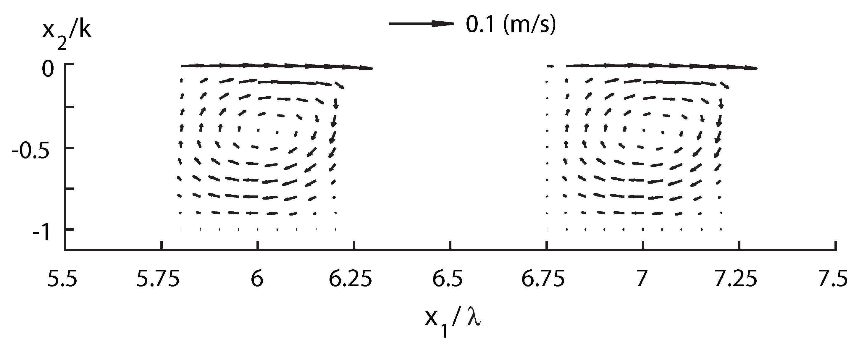
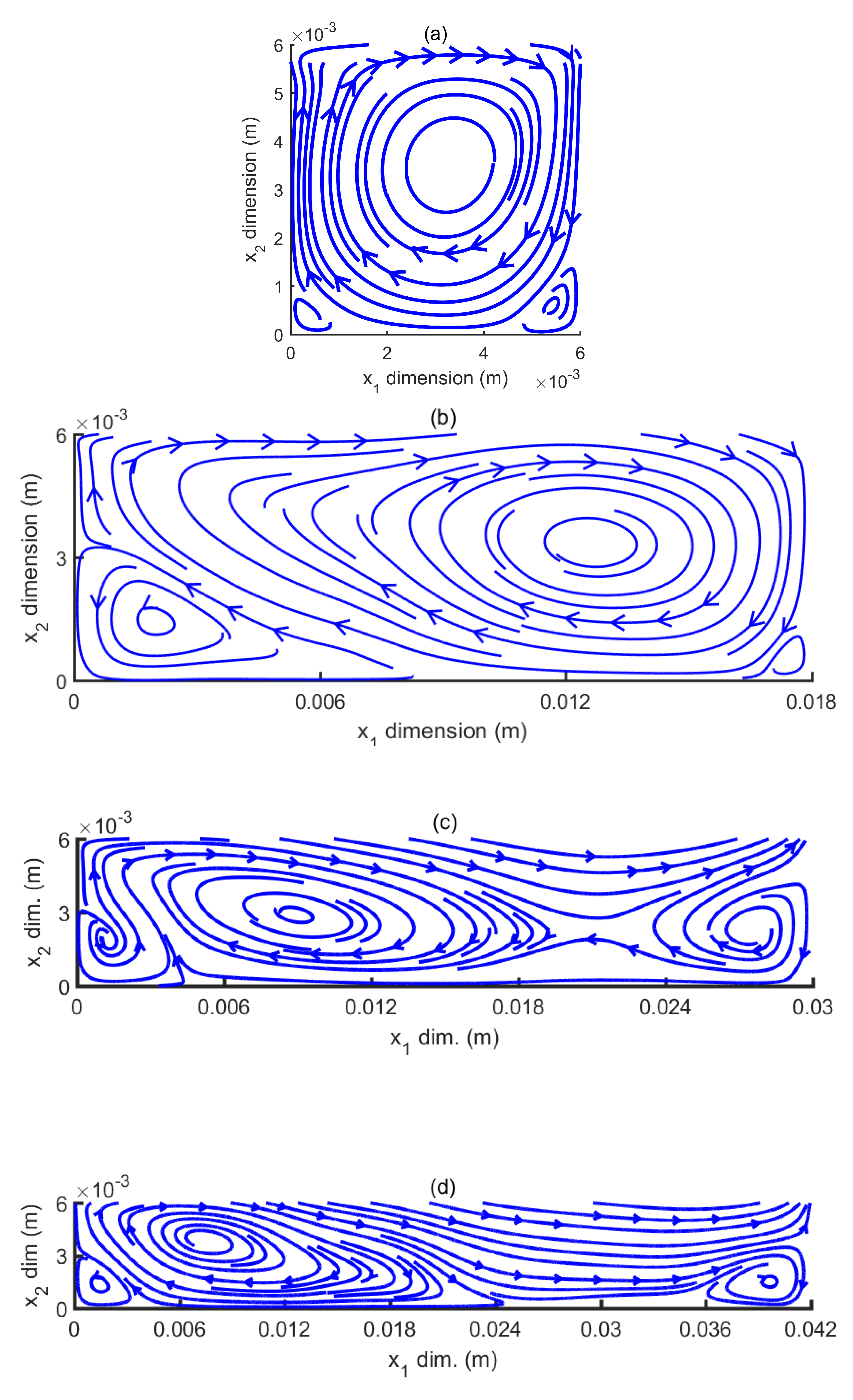
As an example of useful results from LES, streamlines of the predicted mean flows for Runs 1 to 4 are presented in Figure 18a–d. Among the flow fields for the four runs, the major similarities and differences are:

• One similarity was that the flows were all complicated in the cavity, where multiple eddies were present, with different sizes and rotation directions, depending on the spacing of roughness elements.
• Another similarity was that the flows all showed a large clockwise vortex and a small anticlockwise vortex on the left in the cavity. The vertical dimension of the large vortex was limited by the roughness height. The vertical dimension of the small vortex was limited to one half the roughness height.
• One difference was the elongation of the larger vortex. Its aspect ratio (the height in the $x_2$-direction to the width in the $x_1$-direction) appeared to be limited to 1 to 3 (or 1 vertical-to-3 horizontal).
• Another difference was the generation of a vortex on the right.

The LES results reveal great amounts of flow details, which would be technically challenging to measure in experiments. Further analysis of the mean flow and turbulence details would help reveal the dynamic interaction between the outer region and roughness cavity. The current knowledge about the interaction is incomplete.

At $\lambda /k=2$, the mean flow of the outer region seemed to be isolated from the eddy motion in the cavity (Figure 18a). This feature was reported previously in the literature. It’s worth noting that one needs to take into account the turbulence fluctuations near the roughness-top plane in analyses of fluid circulations in the outer region and the cavity. Computational models based on the Reynolds averaged continuity and momentum equations would encounter difficulties in capturing such turbulence fluctuations. Two minor eddies appeared below the main eddy: one in the lower left corner and the other in the lower right corner of the cavity (Figure 18a). Minor eddies also appeared at other values of the $\lambda /k$ (Figure 18b–d). The fluid circulation associated with these minor eddies may be insignificant. However, their presence makes it technical difficult to apply the experimental approach to the delineation of main eddies.

As the ratio $\lambda /k$ increased, the main eddies in the cavity evolved in shape, from being relatively circular (Figure 18a) to more elongated (Figure 18d). As expected, the associated fluid circulations are always in direction aligning with the outer flow in the roughness height plane. The outer-region flow is the energy source for the cavity eddy motion. The main eddies were asymmetrical about their centers, with distortions on either the right side to the left side. 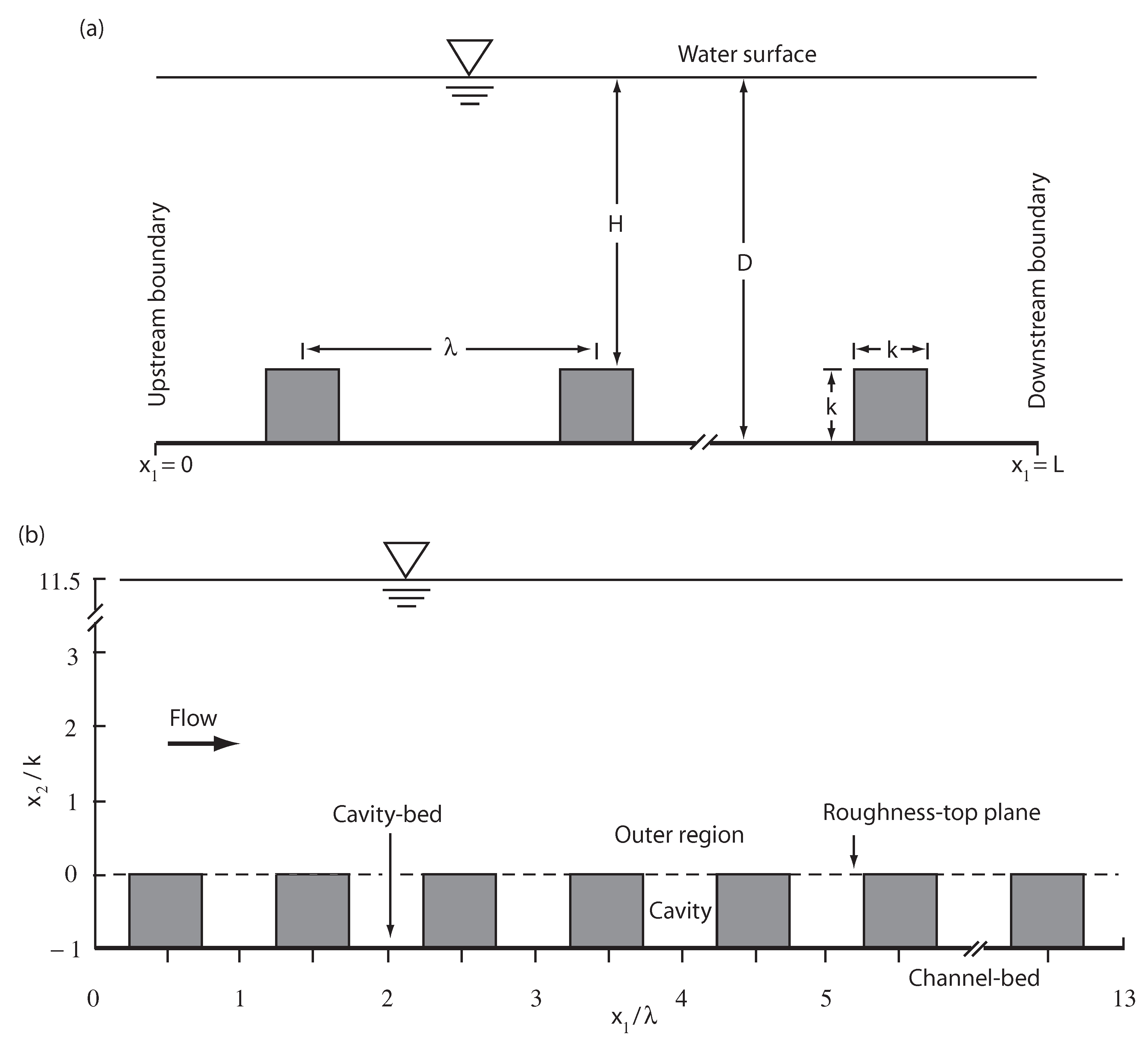They appeared to hug the upstream face of the downstream bar at lower $\lambda /k$ values and the downstream face of the upstream bar at higher $\lambda /k$ values. There were flow separations from the cavity bed (Figure 1) due to eddy motion. An increase of $\lambda /k$ caused eddy motion to deepen and to have more significant contact with the cavity bed. One implication would be an increased potential to erode the bed of a natural open channel.

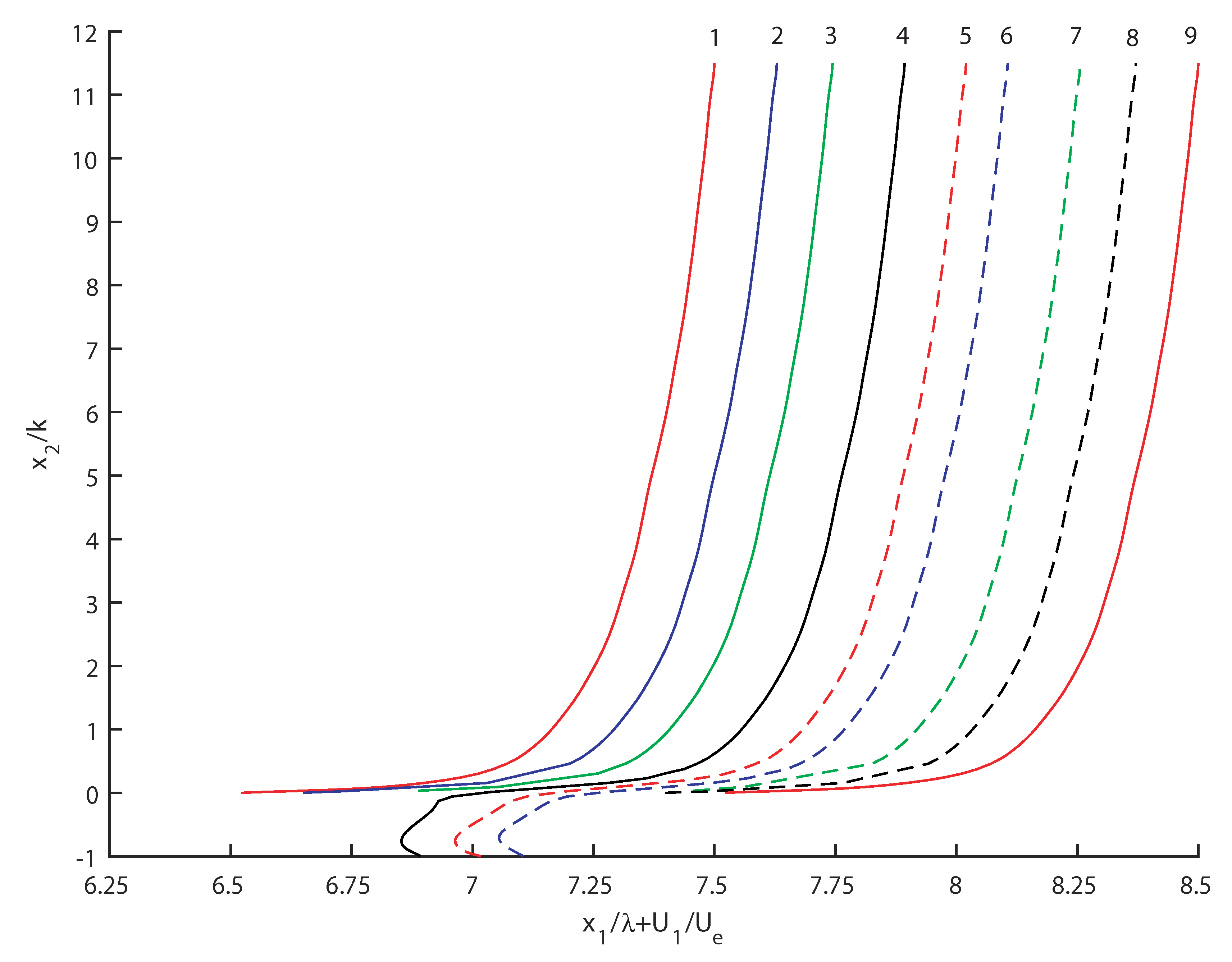
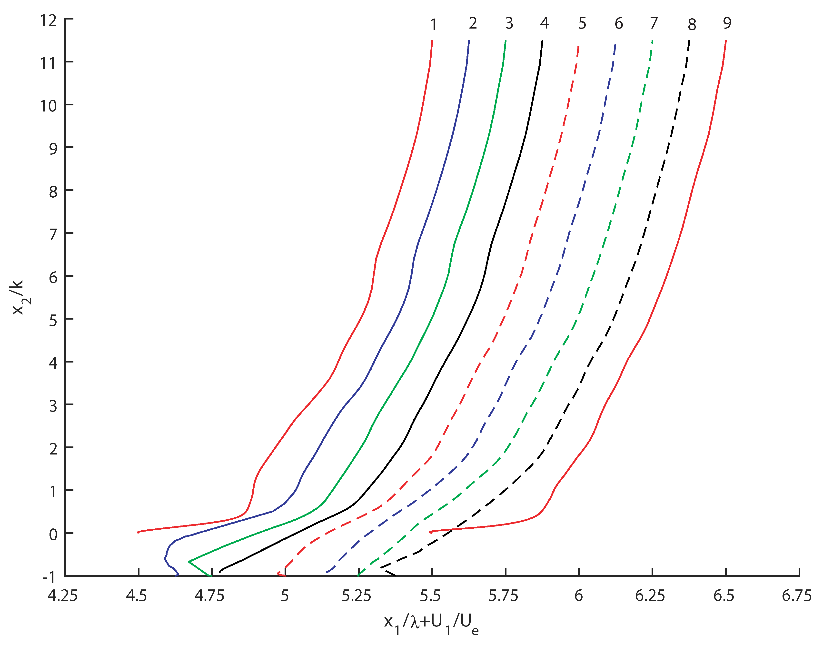
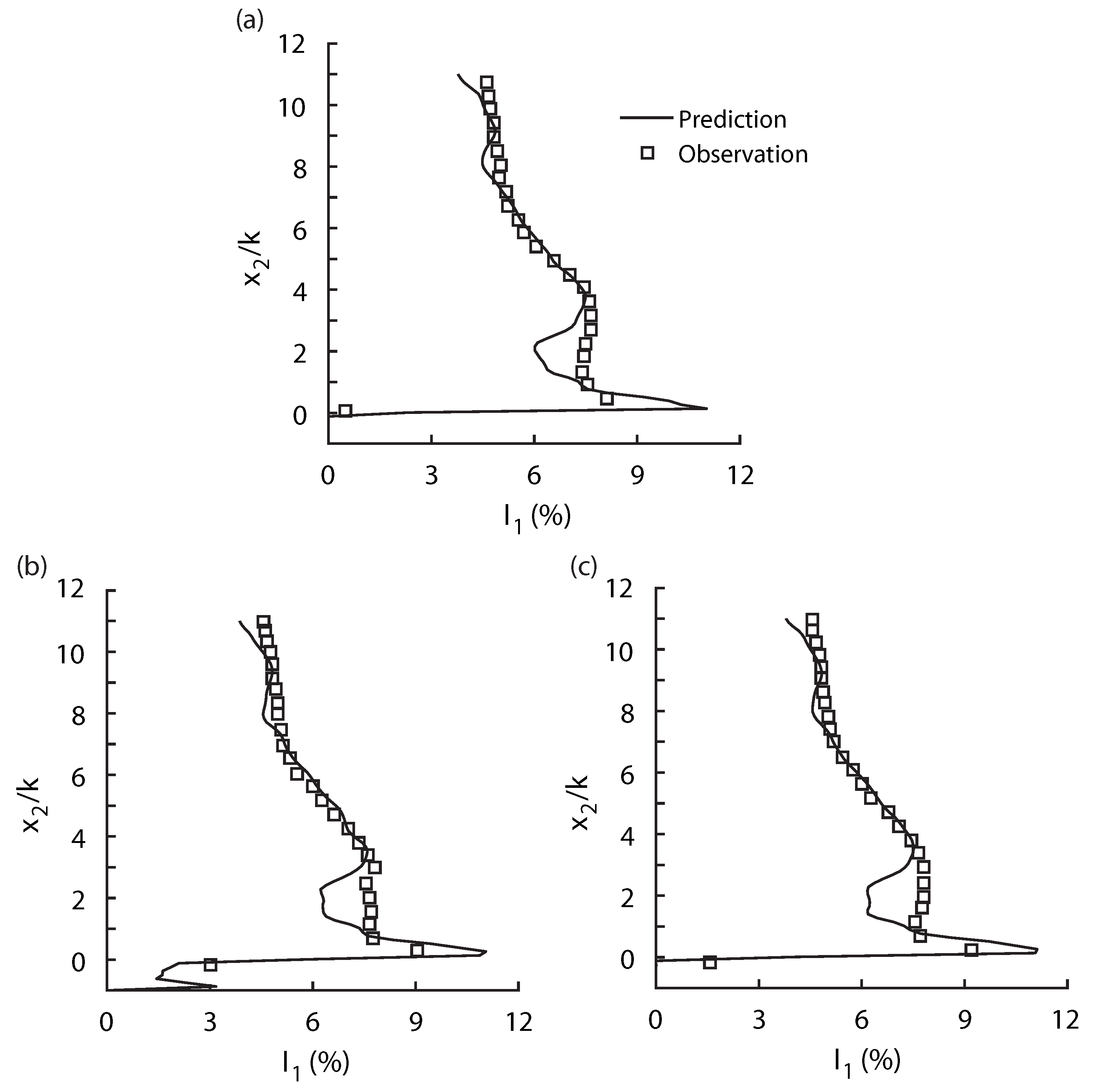
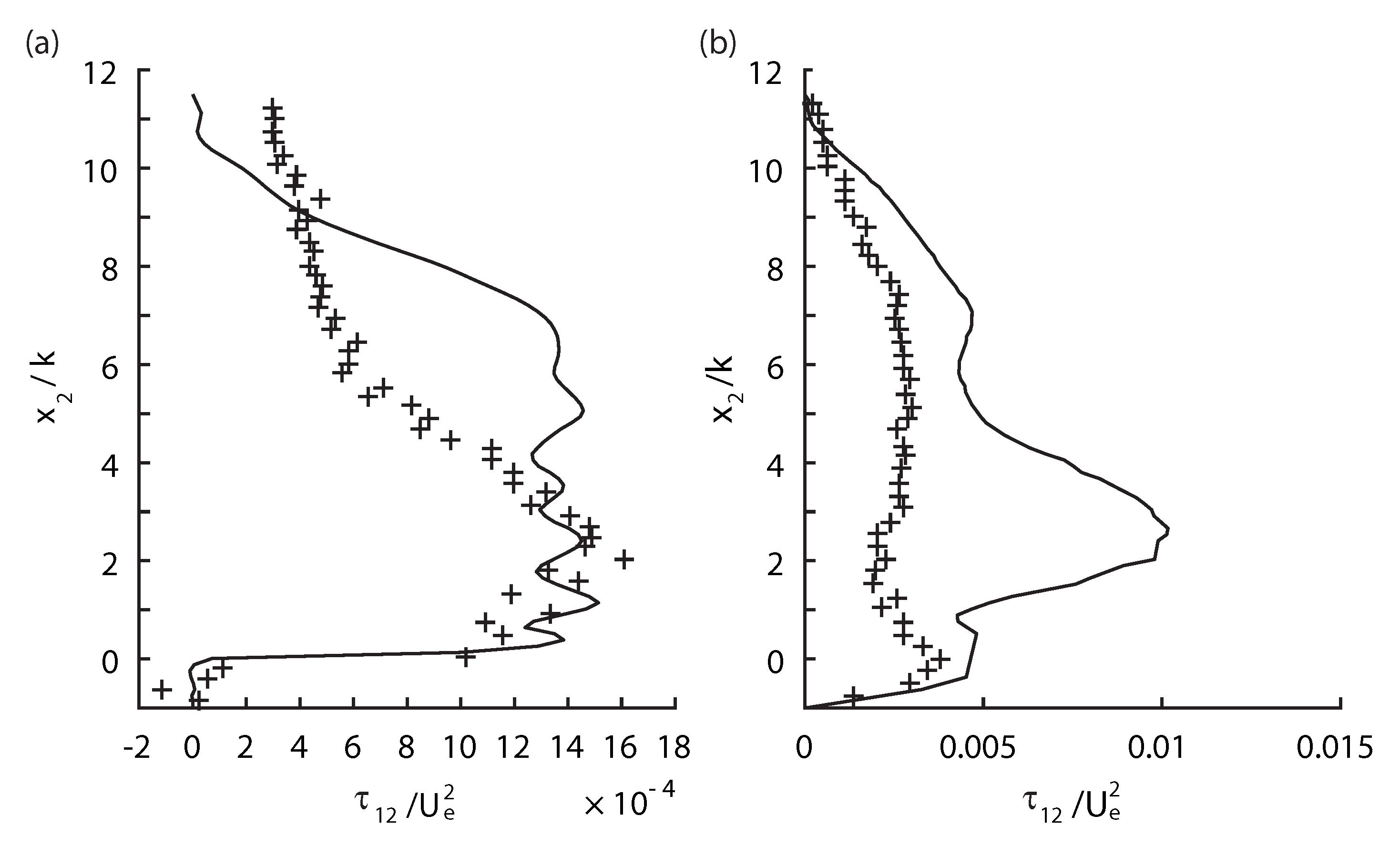
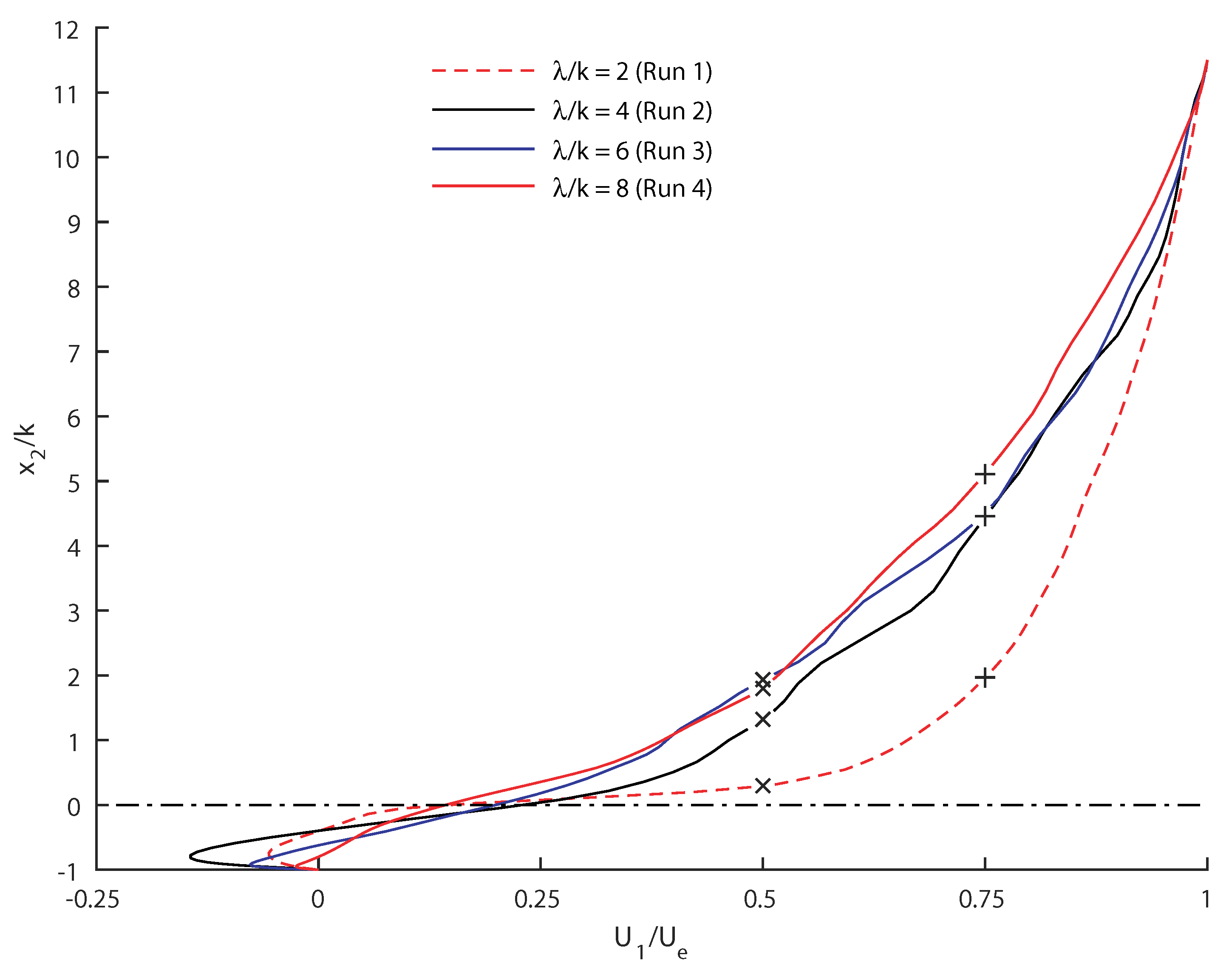
Profile 5 of $U_1/U_e$ in Figure 3 and Figure 14, profile 4 in Figure 15, and profile 5 in Figure 6 are from verticals through the middle between two adjacent roughness elements. The four profiles correspond to $\lambda /k$ = 2, 4, 6, and 8 for Runs 1, 2, 3, and 4, respectively. The profiles are re-plotted in Figure 19 to facilitate a comparison, as an example to quantify the influence of eddy motion in the cavity on the outer flow. In Figure 19, it is shown that at the roughness height ($x_2=0$), the values of $U_1/U_e$ differ among the four runs, being 0.15, 0.23, 0.20, and 0.14, respectively. At other heights $x_2$ > 0, the values of $U_1/U_e$ also differ. 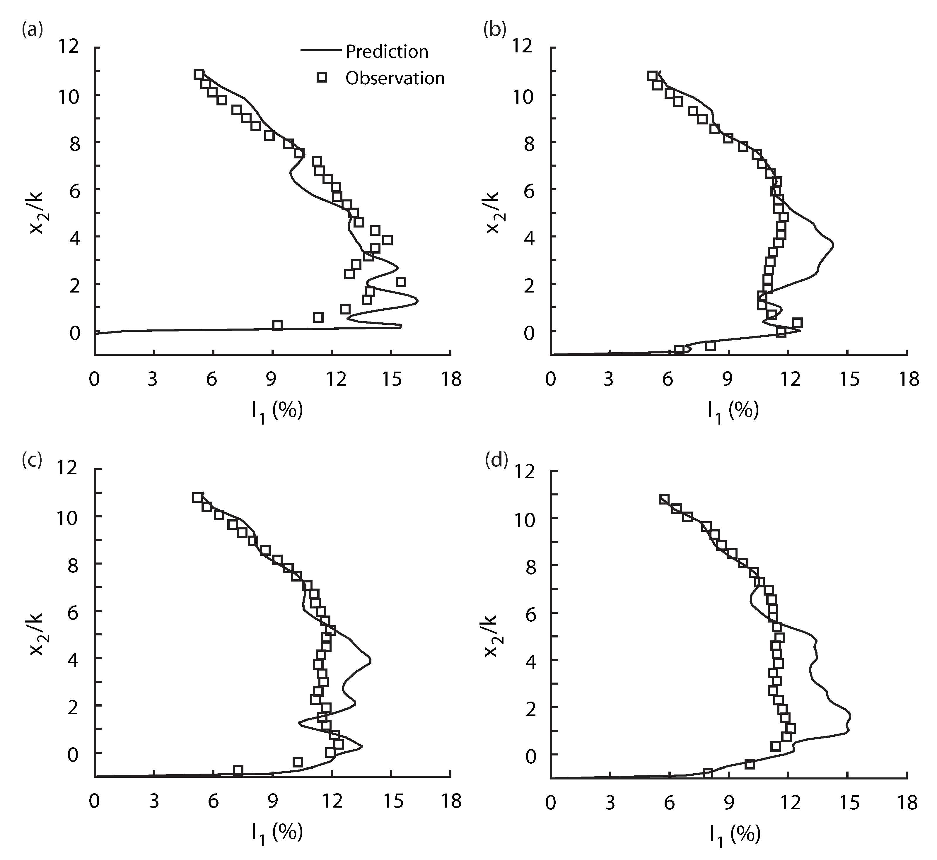For example, at $x_2/k=1$, $U_1/U_e$ are not the same, being 0.66, 0.46, 0.39, and 0.39 for Runs 1, 2, 3, and 4, respectively. In Figure 19, it is shown that $U_1$ reaches 50%$U_e$ (the X markers) and 75%$U_e$ (the plus signs) at a lower height (or a smaller positive $x_2$ value) for Run 1 than the other runs. The above-mentioned differences in $U_1$ are due to the different $\lambda /k$ ratios.

Previously, LES studies of turbulent flow in a conduit with roughness elements on one wall have mostly dealt with air flow in pipes [31,32,33,34]. Pipe flow has a fixed cross section. Open-channel flow has a free surface. Chow [11] pointed out that it is much more difficult to solve problems of flow in open channels than in pressure pipes. For open-channel applications, some researchers (e.g., [35]) have conducted LES of flow over dunes in open channels. Xie et al. [35] investigated the effect of water surface treatments (the volume of fluid method and rigid lid approximation) on flow characteristics. They concluded that the two treatments gave similar mean-flow velocities. Between the two methods, they suggested very slight discrepancies for streamwise and vertical turbulence intensities and the Reynolds stresses in the region below the water surface. In this study of shallow open-channel flow, the boundary layer thickness was a large portion of the total depth, as can be seen from the velocity profiles in Figure 3 and Figure 6, and the ratio of the flow depth to roughness height was small ($H/k=12.5$). In shallow open-channel flows, turbulence fluctuations in the water column can play the role to transmit the dynamic influence of bed roughness on the near-surface flow. This would make the rigid lid approximation less applicable and more likely to introduce artificial effects.

One limitation of this paper is that only two-dimensional roughness elements have been considered. In reality, roughness elements in natural open channels are typically three-dimensional objects. Perhaps the simplest way to create a rough channel-bed with three-dimensional roughness elements is to place cubes on a flat plate. It would be valuable to carry out LES studies of turbulence over such rough beds. Water-surface wave motion or secondary flow in open-channels will cause non-zero vertical velocities near the water surface. To capture vertical motion in the upper water column, future LES models should treat water as the liquid phase and air as the gas phase. It is understood that two-phase flow LES will incur much higher computing costs.

5. Conclusions

This paper has presented LES results of the mean-flow as well as turbulence quantities for flow in rough open-channels, along with validations of some of the results using available experimental data [13]. The bed roughness is created by placing transverse square bars at the otherwise flat channel-bed. The longitudinal spacing of the evenly placed bars ranges from $\lambda /k=2$ to 8 (the ratio of pitch to roughness height); the two limiting values correspond to the d-type of roughness and the k-type of roughness, for which experimental data are available for comparison. This LES study has included two transitional cases with the ratio $\lambda /k$ between 2 and 8, which demonstrates the complement of efficient LES modeling to expensive laboratory experiments. The LES results have been shown to be of satisfactory accuracy. Analysis of the LES results leads to the following conclusions:

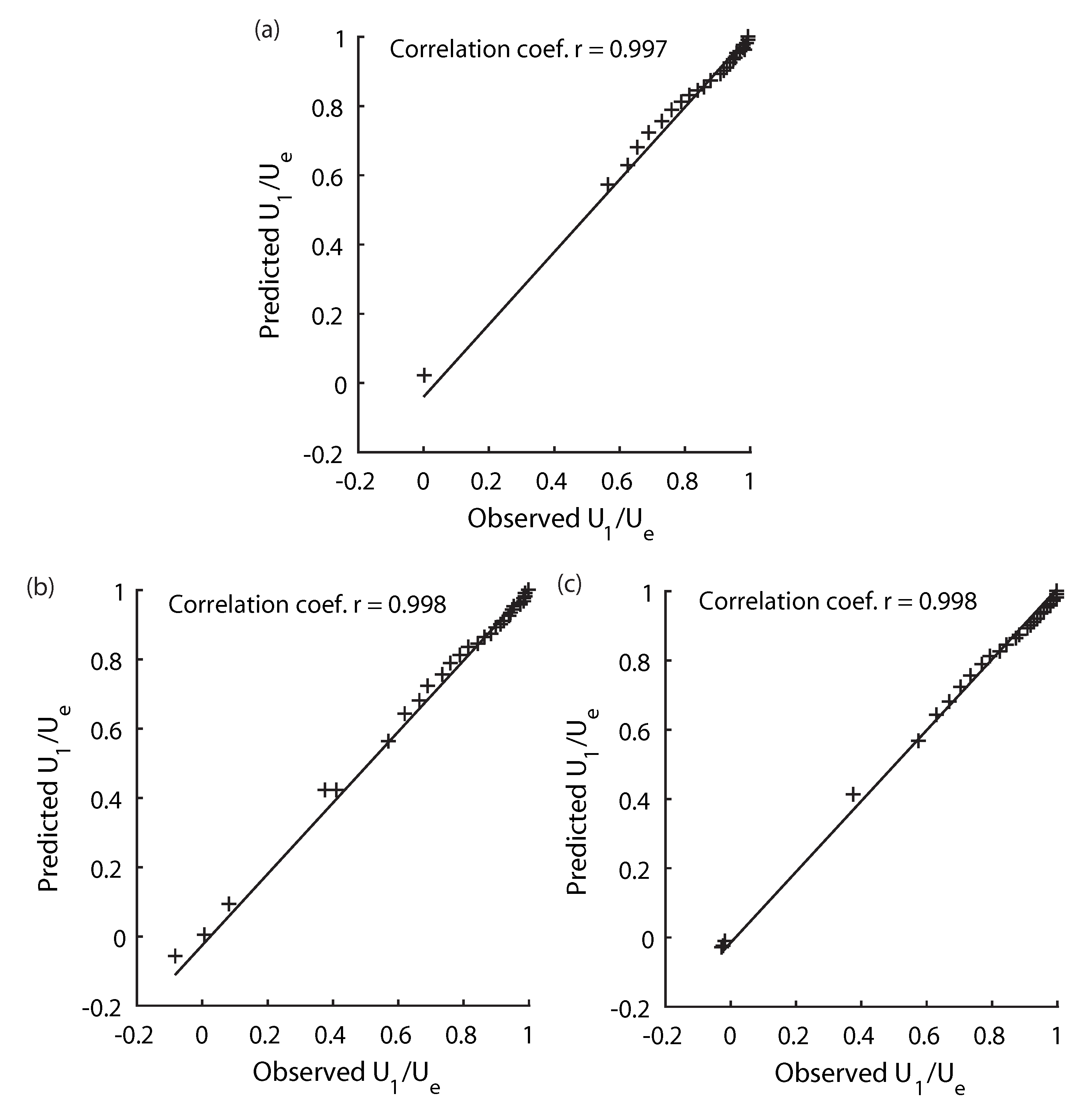
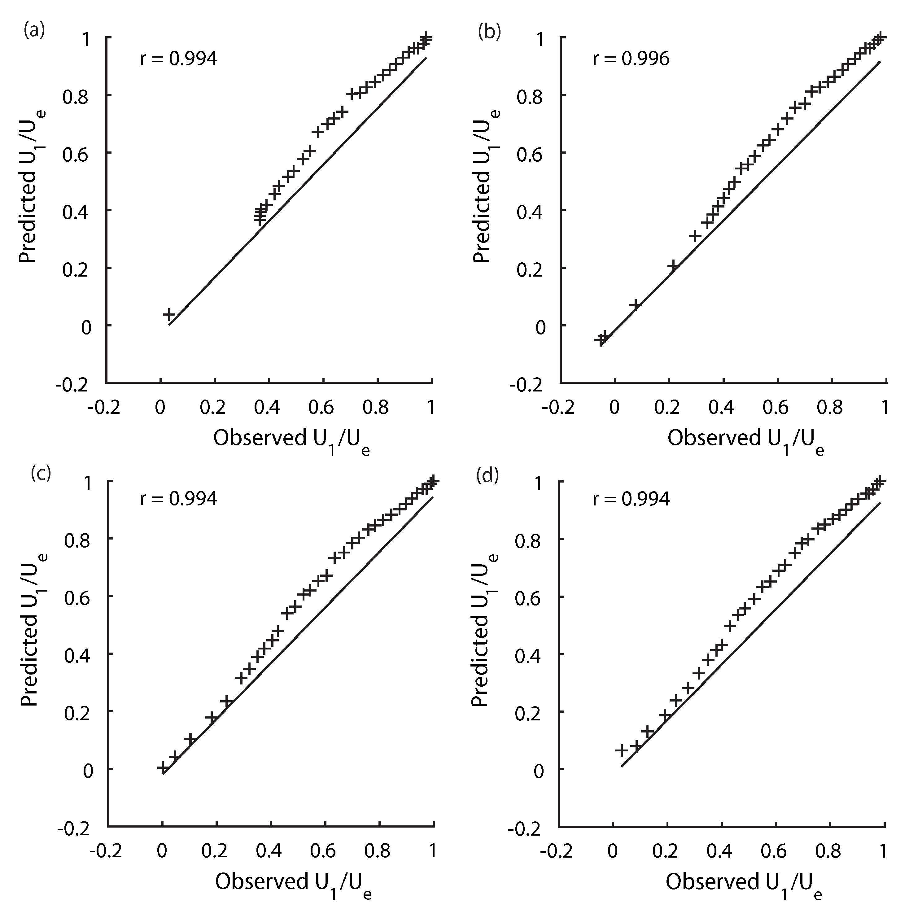
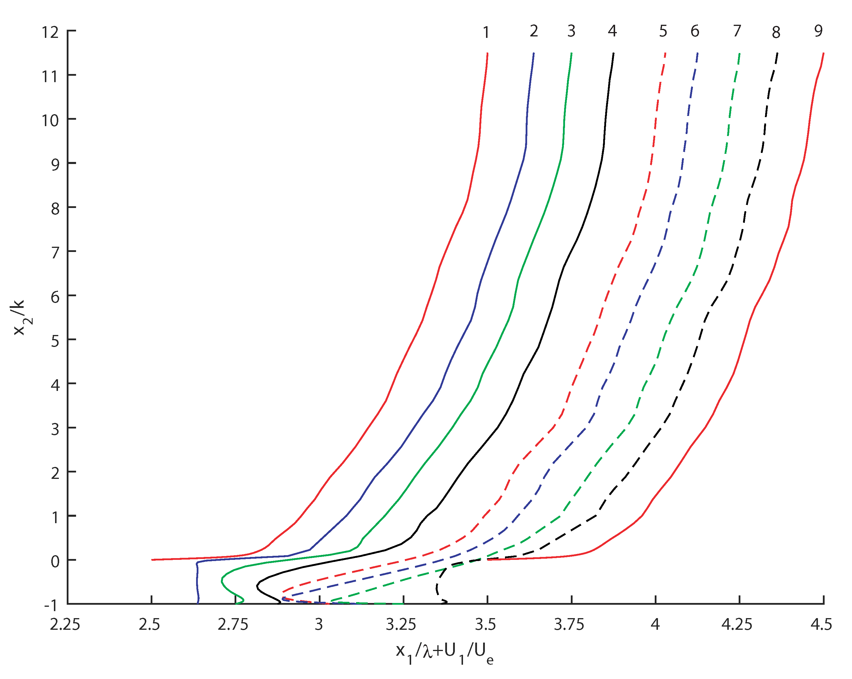
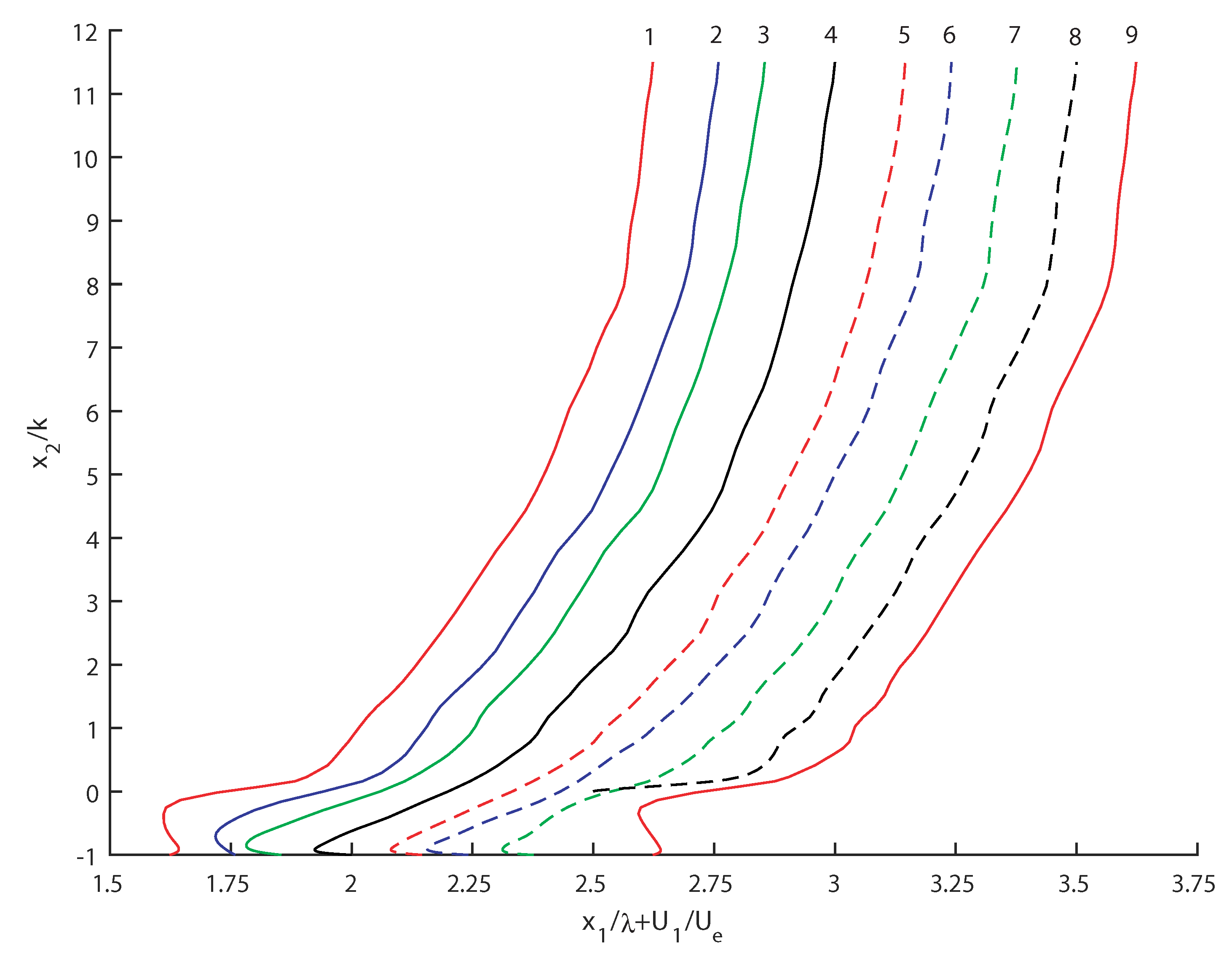
At $\lambda /k=2$, vertical profiles of the mean-flow velocity component in the streamwise direction resemble those in the classic turbulent boundary layer over a flat plate, except there is a certain vertical shift, depending on the proximity to roughness elements. At $\lambda /k=8$, the mean-flow velocity profiles display changing patterns in the vicinity of roughness elements. In both cases, the velocity profiles show bottom boundary layers to constitute a large portion of the total depth. Thus, the bed roughness influences the flow throughout the shallow water column up to the water surface. This condition reduces the applicability of the rigid lid approximation in LES modeling of shallow open-channel flows over roughness elements.

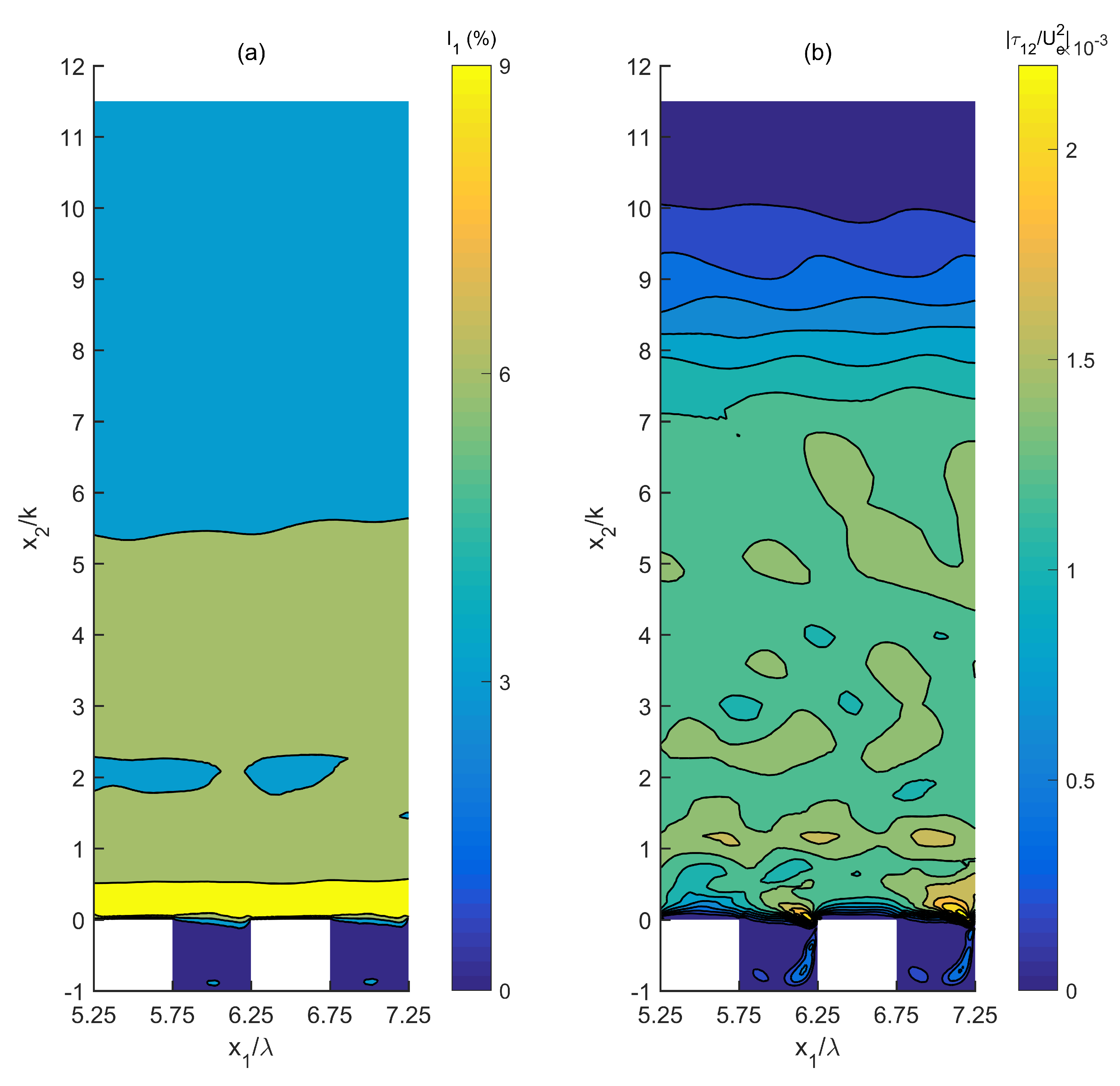
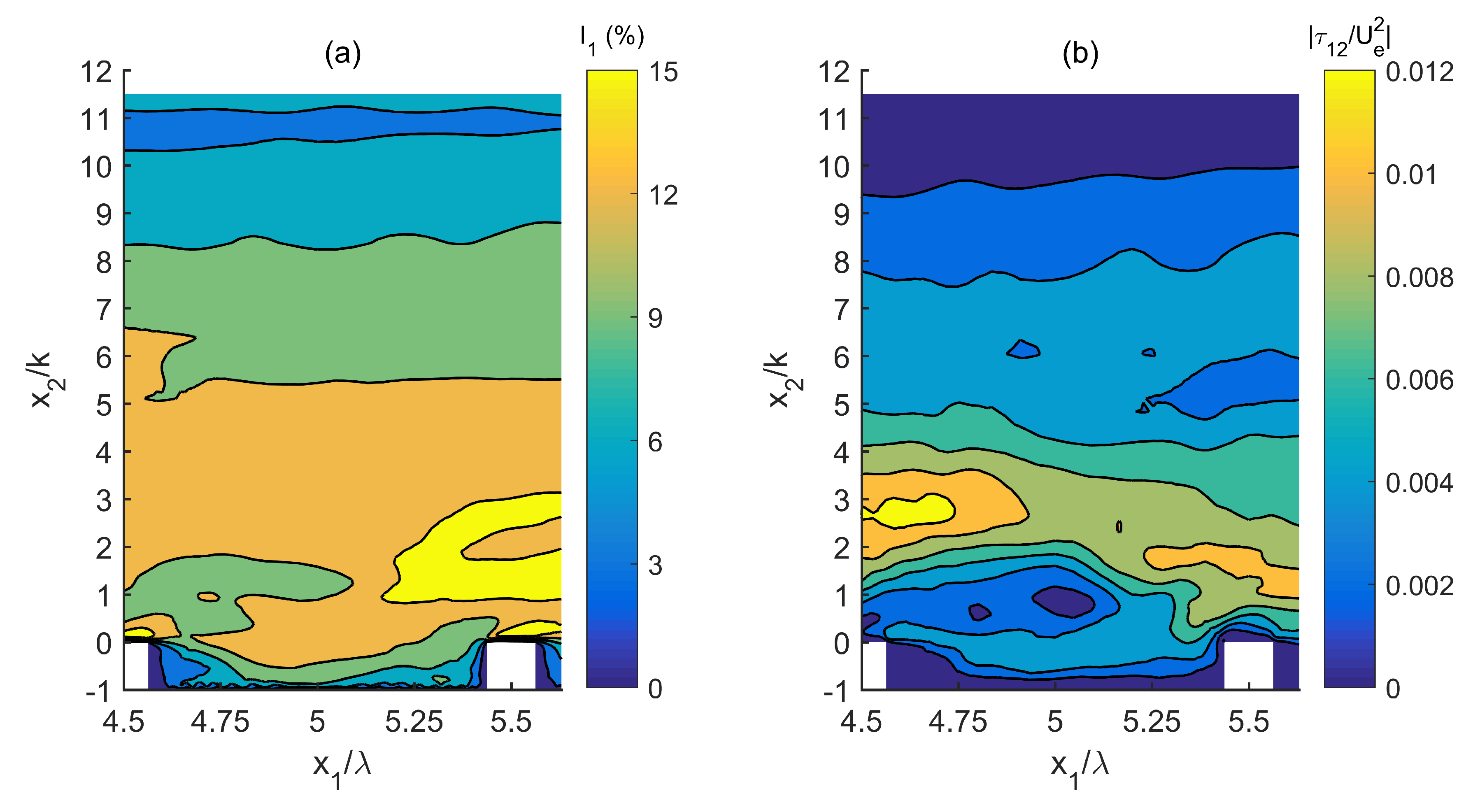
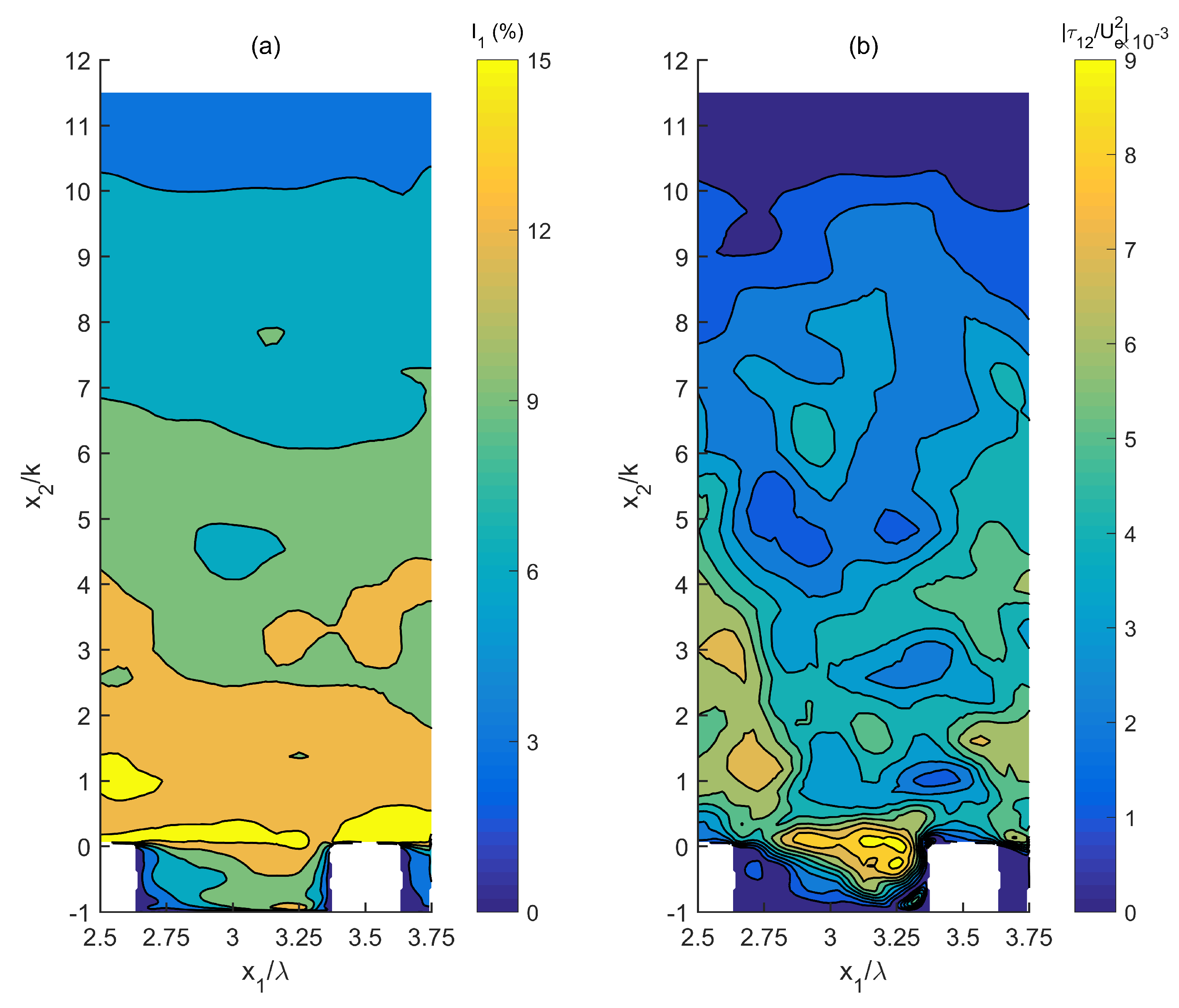
In both the d-type and the k-type of roughness, fluid mass exchanges between the roughness cavity and the outer region due to turbulence fluctuations near the roughness height plane. The k-type of roughness causes stronger intensities of turbulence fluctuations in both the streamwise and vertical directions than the d-type of roughness. For the d-type of roughness, vertical profiles of the intensity of streamwise turbulence fluctuations are more or less the same, regardless of the longitudinal position relative to roughness elements, whereas, for the k-type of roughness, the profiles are somewhat different from one location to another. The ratio $\lambda /k$ dictates the number of eddies in the cavity between two adjacent bars as well as the eddies’ locations and shapes. The ratio also has profound influence on the shear stress field.

In all the cases of $\lambda /k$ considered in this paper, the flows in the cavity are complicated, with the occurrence of a large clockwise vortex and a small anticlockwise vortex on the left. Relatively large $\lambda /k$ ratios tend to cause elongation of the larger vortex and create an additional vortex on the right.