Article

The Use of Various Rainfall Simulators in the Determination of the Driving Forces of Changes in Sediment Concentration and Clay Enrichment

1
Geographical Institute, Research Centre for Astronomy and Earth Sciences, 1112 Budapest, Hungary
2
Department of Nature Conservation and Landscape Ecology, Faculty of Agricultural and Environmental Sciences, Szent István University, 2100 Gödöllő, Hungary
3
Institute for Geological and Geochemical Research, Research Centre for Astronomy and Earth Sciences, 1112 Budapest, Hungary
4
Institute of Geography and Geoinformatics, University of Miskolc, 3515 Miskolc, Hungary
5
Department of Environmental and Landscape Geography, ELTE University, 1117 Budapest, Hungary
*
Author to whom correspondence should be addressed.
Water 2020, 12(10), 2856; https://doi.org/10.3390/w12102856
Submission received: 10 September 2020 / Revised: 8 October 2020 / Accepted: 10 October 2020 / Published: 14 October 2020
(This article belongs to the Special Issue Soil Water Erosion)

Abstract

:
Soil erosion is a complex, destructive process that endangers food security in many parts of the world; thus, its investigation is a key issue. While the measurement of interrill erosion is a necessity, the methods used to carry it out vary greatly, and the comparison of the results is often difficult. The present study aimed to examine the results of two rainfall simulators, testing their sensitivity to different environmental conditions. Plot-scale nozzle type rainfall simulation experiments were conducted on the same regosol under both field and laboratory conditions to compare the dominant driving factors of runoff and soil loss. In the course of the experiments, high-intensity rainfall, various slope gradients, and different soil surface states (moisture content, roughness, and crust state) were chosen as the response parameters, and their driving factors were sought. In terms of the overall erosion process, the runoff, and soil loss properties, we found an agreement between the simulators. However, in the field (a 6 m2 plot), the sediment concentration was related to the soil conditions and therefore its hydrological properties, whereas in the laboratory (a 0.5 m2 plot), slope steepness and rainfall intensity were the main driving factors. This, in turn, indicates that the design of a rainfall simulator may affect the results of the research it is intended for, even if the differences occasioned by various designs may be of a low order.

1. Introduction

Preventing soil erosion is one of the most significant environmental challenges that an increasing global population has to face. Consequently, understanding the infiltration and soil erosion process is a key task, and has generated a wide range of investigations [1].
Concerning interrill erosion, the most commonly regarded drivers are slope gradient, porosity, canopy cover rate (the ratio of the soil surface covered by plants reducing the impact of splash erosion), surface roughness, soil moisture, and organic matter content, including soil texture as representative of surface conditions [2,3,4,5]. The other group of driver factors is precipitation-related, including elements such as intensity, uniformity, drop size distribution, and kinetic energy. Taking such driver parameters into account, studies aim to determine response properties, such as the quantity of eroded sediment [6], temporal variation in runoff discharge and sediment concentration [7], or the aggregate size [8] and particle size distribution (PSD) of the eroded sediment [9,10,11] in the contexts of organic carbon [12] and nutrient loss [13].
A challenge faced by any soil erosion study is that the combined effects of these factors and parameters create a dynamic and complex system of driving factors [14]. Even though the considerable amount of data collected and measured provides a stable basis for the construction of models and the models employed have become more precise, further measurements are still needed to deepen our understanding [15]. As environmental circumstances (soil, canopy cover, tillage operations, rainfall properties, etc.) vary across a wide spectrum, in the interests of comparability, rainfall simulation was introduced. With the application of rainfall simulation, most precipitation-related properties can be standardized, even though the results thus obtained may be affected by the research design selected [16]. In the present study, the term “rainfall simulator” refers to the applied research design including the entire measurement system. Both field and laboratory rainfall simulators are widely used for modeling eroded environments [17,18,19,20]. They are useful for understanding the parameters and interactions influencing sediment transport and selective mechanisms under interrill erosion.
Although a large number of rainfall simulation studies have been conducted in the recent past, only a few have compared simulator efficiency [14,21,22,23], making the comparison of studies conducted using different kinds of simulators difficult. Moreover, the changes in the scale of the research, from point to catchment, typically affect the sediment yield results [1]. In the <m2 scale, the absence of linear erosion generally mitigates specific soil loss even though the increase of research sites triggers decreasing specific soil loss due to sedimentation within the plot.
The present study, therefore, aimed to examine and compare the measured properties of the same soil under different surface conditions (moisture content, slope gradient, and crust conditions) using both field and laboratory rainfall simulations. Intensive rainfall and location-specific methodology were used at two sites. The main hydrological properties (time to ponding and ponding period, time to runoff, runoff-to-infiltration ratio, and the characteristics of runoff after precipitation), sediment concentration, and clay enrichment were the basis of the comparison. The time to runoff is a key element in the pre-runoff phase, as it decreases with increasing rainfall intensity and, at least generally, decreases with increasing slope gradient [24] and higher initial soil moisture content [7]. Sediment concentration was selected because, according to Iserloh et al. and Chaplot and Bissonnais [22,25], it is able to represent soil loss and susceptibility to erosion well, but is independent of the length of rainfall, and can therefore be used as a comparative value during multi-simulator studies. On the basis of the results of Warrington et al. [9], the preferential loss of clay and its enrichment, compared to the original soil, in runoff was found to be important in erosion control as most of the plant-available nutrients as well as the soil organic matter and thus the buffer capacity and aggregate stability of the soil are related to the clay fraction. Beyond making a simple comparison, the idea was to summarize the results of the single parameters into a complex property (approach), which is relevant to the method applied. The following specific objectives were thus pursued: (i) to determine the similarities and differences between the soil properties measured in the two experiments; (ii) to identify the reasons for any differences; and (iii) beyond the single properties, to attempt to find a complex approach that would make the comparison of the simulators possible.

2. Material and Methods

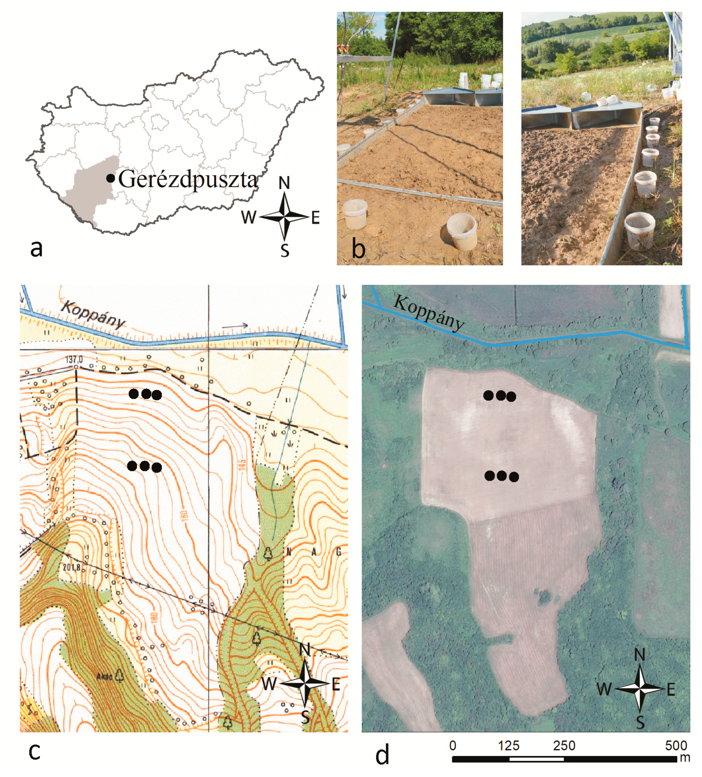
2.1. Study Area and Soil Properties

The field experiments were conducted near Gerézdpuszta, situated in the Koppány Valley adjacent to the floodplain of the Koppány River (Figure 1). This area is located in the east of the Somogy Region, southwest Hungary.
Owing to the loess-like deposits, the area is prone to severe soil erosion; however, a further impact on the soil is the reason why conventional tillage has become less popular in recent decades [26]. The hillslopes that are less eroded due to the lack of tillage are characterized by Cambisols, while mostly Regosols and Colluviums can be found in the cultivated areas [27]. The climate is moderately warm and wet, with an average annual temperature of 10.0–10.2 °C and average annual precipitation of 605–700 mm. Most of the hillsides are characterized by agricultural cultivation, almost half of which is situated on slopes steeper than 12% [28]. The consequent tillage depths have resulted in hard plough-pan with extremely low porosity and infiltration.
The field experiments and the sampling for the laboratory investigations were conducted on recently tilled (seedbed preparation) Regosol, which had a silty clay loam texture, as well as low CaCO3 and organic carbon contents (Table 1).
Field rainfall simulations were carried out on plots that were 3 m in length and 2 m in width, in triplicate. Altogether, 6 plots were investigated: 3 on the gentler parts of the slope (with an incline of 7–8%), and 3 on steeper parts (17–18%) (see Appendix A). The plots on the same parts of the slope were placed 2–3 m from each other (Figure 1). The soil samples for laboratory simulations (from the topmost 0–25 cm tilled layer) were collected from the site at which the in situ simulations were conducted. In the laboratory, the collected samples were loaded into the flume in the state in which they had arrived. Initially, the flume was covered by woven geotextiles to ensure free drainage through the flume bottom to the collector taps. The soil was compacted solely by the energy of two successive (simulated) rainfall events (30 mm) to achieve the 20 cm soil depth required for the investigations. To exclude the effects of splash erosion, we covered the soil surface by a polyethylene mesh during these compaction pretreatments.

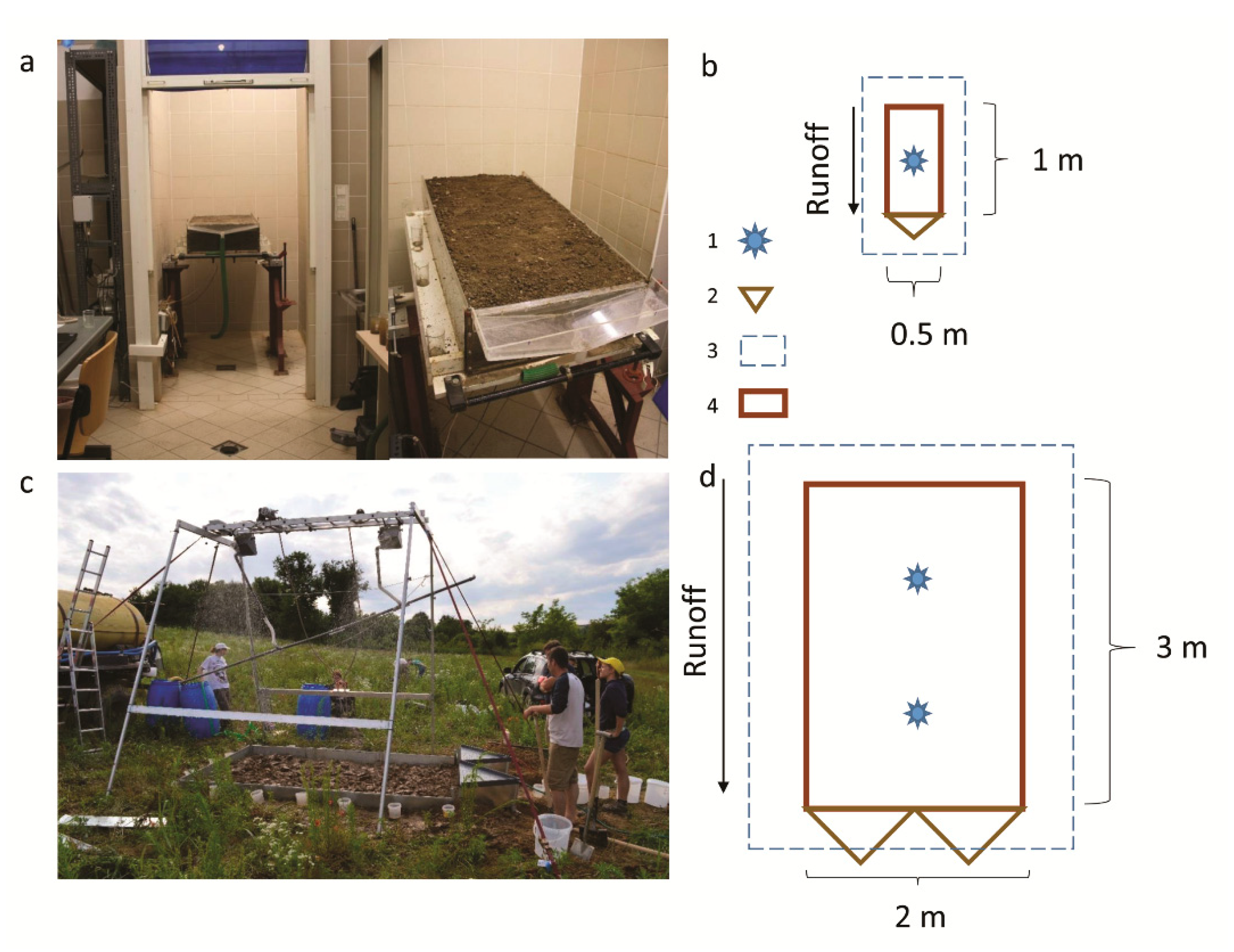
2.2. Rainfall Simulators Used in the Study

Two rainfall simulators were used in the experiment, the Shower Power (SP) and the “ELTE” simulator. SP 02 is a frequently used [29,30], portable field unit that can be employed at the plot-scale with alternating nozzles (Figure 2a,b). The device has a plot of 3 × 2 m; however, in this instance, the irrigated plot size was 12 m2 to exclude border effects [30]. The drop forming unit, at a height of 3 m, comprises an alternating axis equipped with two adjacent 80100 Veejet nozzles spaced at 2 m [31]. This distance ensures complete overlap between the two nozzles to gain a uniform spatial intensity and drop size distribution pattern. The intensity can be set to 30–100 mm h−1, depending on the axis alternation frequency. The average kinetic energy of the simulator is 24 J m−2 mm−1, ensuring a reasonable drop size distribution and kinetic energy simulation of an intense natural rain [31]. Field measurement results are presented in Table A1. The properties affecting the momentary intensity and drop spectrum during a simulation (pressure regulation, evaporation, wind, pump properties) may well vary in the field, causing anomalies in the preset intensity and kinetic energy [32]. Thus, it was the real, independently measured rainfall intensities that had been collected (an average for each single run) that were used for calculations instead of the preset ones.
The ELTE simulator [33,34] is a point-scale laboratory device equipped with a fixed 1/2 HH 40 WSQ full-cone nozzle (Figure 2c,d). It was set at a height of 3 m using a constant pressure of 20 kPa, which created a standard intensity of 80 mm h−1, with an average kinetic energy of 17 J m−2 mm−1, well representing the effects of an intense natural rainfall [35]. The ELTE simulator has a sample/monolith carrier flume measuring (lwd) 100 × 50 × 20 cm. The steepness of the monolith can be regulated over a range of 0–100%. On the bottom of the flume, under the geotextile cover, a collector system is fitted to drain the leaching water through four taps. In the present investigation, each tap was closed, modelling the quasi impermeable plough-pan layer detected in the field and thus increasing/maximizing the comparability of the research design of the field and laboratory measurements. This research design does not take the effect of splash out (runoff and sediment loss due to raindrop reflex from the surface, which leave the flume across the borders) into account, causing lower runoff and sediment yield values.

2.3. Experimental Design

A total of 18 simulation runs were conducted: 12 in the field and 6 in the laboratory (Table 2). As the soil was the same, the impact of rainfall intensity, slope gradient, and soil surface parameters (roughness, moisture content, and crust state) on soil loss could be examined. The notion of the comparability of the erosion observed in the 2 experiments (comparing an in situ soil to a transported disturbed soil sample) was based on conclusions reached by Thomaz and Pereira [36], who found that the hydro-erosional responses of soils in a conventional tillage system or unstructured soils are similar.
A gentle slope of 5% was set in the laboratory, whereas all values <10% were classified as gentle in the field. The steep slope in the laboratory measurements was 12%, while slopes >10% were considered as steep in the field. Due to the dynamic nature of variable changes in surface roughness and moisture content under the effects of precipitation, we conducted 8 dual experiments, resulting in a total of 16 simulations. The first simulation runs (FG1; FG3; FG5; FS1; FS3; FS5; LG1; LS1) modeled the seedbed (recently tilled, relatively dry) soil with a rough surface, and the second runs (FG2; FG4; FG6; FS2; FS4; FS6; LG2; LS2) were conducted over the sealed and smoothed soil with the evolved crust and higher soil moisture content.
In the remaining two laboratory simulations (LP1; LP2), we simulated extremes of moisture content (modeling “drought” and “inland inundation”) on a nearly flat surface (2% slope). A wide moisture content interval was necessary because the soil moisture content is an important factor controlling runoff [37], and its combined effect with the slope gradient could present an increased impact [38].
Four degrees of intensity (55, 70, 80, and 100 mm h−1) were planned and set for the field simulations. To measure the real amount of rainfall reaching, we placed the soil surface collector dishes next to the plot borders. Owing to the changes in evaporation, wind, and fluctuation in water pressure at the nozzles, the intensities as actually measured differed from those that had been set. For calculations, we used the measured amount and intensities. The time was recorded during all simulated rainfalls. All experiments were divided into 4 time periods: (1) time to ponding—in this period the infiltration exceeded rainfall intensity. The length of this period is proportional to the initial infiltration capacity; (2) ponding period (the length of which refers to the water storage capacity of the surface, or, in other words, the surface roughness); (3) runoff; and (4) the post-rain runoff period (runoff after the rain stops)—the length of this period also reflects the volume of water stored on the surface and indicates the degree of spatial connectivity. As the length of the ponding period describes the surface storage capacity, it is therefore an indirect measure of microtopography. During sample collection, all runoff was measured and collected, and runoff volumes were related to time intervals. After precipitation stopped, the runoff was collected into a separate bucket, and its volume was measured. The times at which ponds appeared and the runoff started and ended, as well as the length of runoff time after precipitation ended, were also recorded [29,30].

2.4. Runoff and Soil Loss Characterization

The total amount of soil loss was weighed after drying for 48 h at 60 °C. The sediment concentration (SC) of each sub-sample was calculated as the dry sediment mass per runoff volume (g L−1). The PSD of each sub-sample was determined in triplicate with a laser diffractometer (Horiba LA-950). For the PSD measurements, we selected the Mie theory of light scattering because it is more precise in the determination of clay fractions than Fraunhofer diffraction [39]. The refractive indices (RI) based on the Horiba software calculation were set to 1.63 (real RI) and 0.3 (imaginary RI).
The constant runoff rate was calculated using linear regression on the measured cumulative runoff volumes with time (practically during the second part of period 3) on the basis of the method described by Jakab et al. [30], in which the steepness of the fitted linear function provides the constant runoff rate (Table A2). The runoff coefficient was determined as the percentage of the constant runoff rate related to rainfall intensity. The clay enrichment CE values of each simulation were calculated as the median clay content values of the sub-samples in relation to the median clay content of the in situ soil. The upper limit for the clay fraction was set at 8 µm [40].

2.5. Statistical Analyses

To obtain an overall picture of the dataset, we produced box and whisker plots. Differences between the parameters of the various laboratory and field samples were calculated using independent samples Mann–Whitney U tests [41], while in other cases when more than 2 groups were compared, an independent samples Kruskal–Wallis test [42] was used. It is difficult to determine the combined impact of the most influential independent variables (e.g., SC) in a complex system. However, in many cases, multivariate statistical tools can assist in resolving such problems. For example, variance analysis has been employed in a study on the effect of rain intensity, slope length, and gradient on SC [25]. As in other studies [43,44,45], principal component analysis (PCA) [46] was used to determine how SC influences response parameters measured in the soil.
In the present study, to explore how soil parameters affect the SC, primary (slope gradient (%), rain intensity (mm h−1)) and derived properties (constant runoff/infiltration (%), ponding period length (s), constant runoff rate (mm h−1)) of the field and laboratory measurements were selected as input parameters for PCA. Since they are all related to hydrology and runoff formation and, furthermore, independent of soil loss, they are suitable for the measurement and prediction of the likely susceptibility of a given soil to erosion, and thus, also, the sole chosen explanatory parameter, SC. The median diameter of the soil that was lost (µm) was also selected as a response parameter, since it also might reflect SC.
Prior to PCA, we conducted Bartlett’s test [47] to investigate the applicability of the input correlation matrices (field and laboratory) to PCA. Both the field ( χ 2 ( 15 ) = 56.63 , p = 9.47 × 10 7 ) and the laboratory datasets ( χ 2 ( 15 ) = 85.87 , p = 5.8 × 10 12 ) were found to be statistically suitable for the application of PCA. Thus, the variability of the variables input to PCA was compressed into principal components on the basis of their linear relationships, as presented by Hatvani [48,49]. It should be noted that the observations’ principal components (PCs) are referred to as PC scores. The elements of the eigenvectors of the empirical correlation matrix will be referred to as loadings, with these measuring the relationship of the coordinates and the PCs with the Pearson correlation coefficient. Loadings outside the ±0.7 interval are considered as meaningful.
During PCA, we took the PCs into account on the basis of their scree plots [50] and their eigenvalues, which had to be above 1 [51]. Thus, taking into account the previous considerations, the input variables’ time series were practically reduced to vectors with uncorrelated coordinates (PC scores) using the first two PCs.
All computations were performed using STATISTICA 10, IBM SPSS 26, R, and visualized in MS Excel 2016.

3. Results

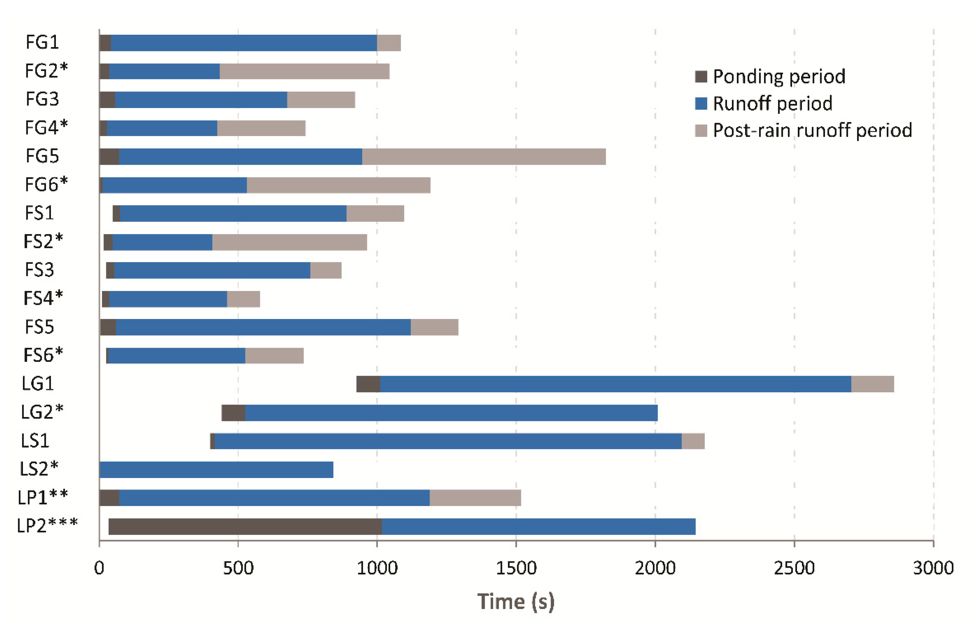
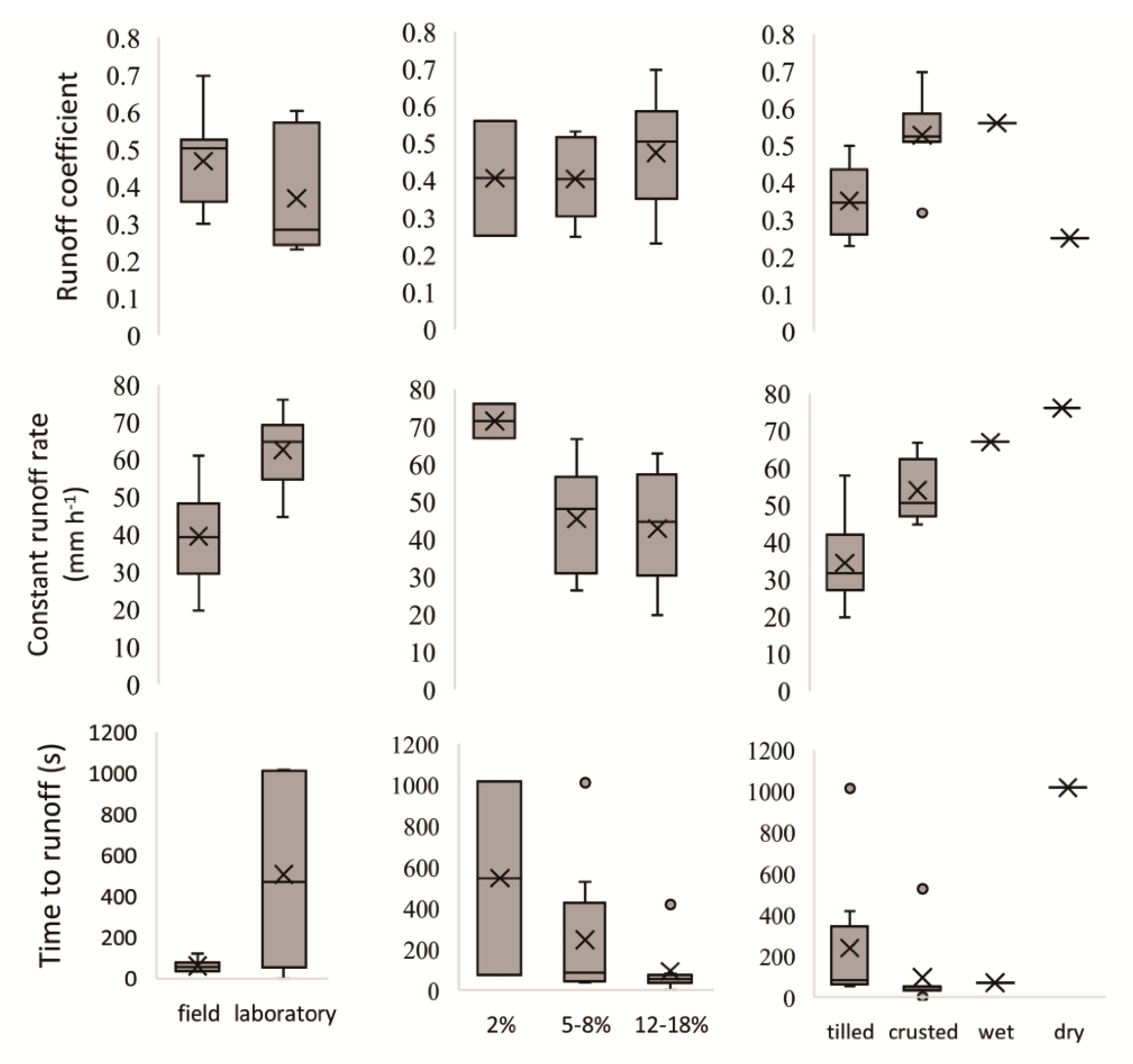
3.1. Variations in Ponding and Runoff Related Properties

Ponding and time to runoff periods did not differ significantly in the lab and the field (U(NField = 12, NLab = 6) = 49, p = 0.25) and (U(NField = 12, NLab = 6) = 56, p = 0.067) at α = 0.05 . However, the duration of runoff and post-rain runoff in the field and the lab were significantly different (U(NField = 12, NLab = 6) = 69 and 11, respectively, p < 0.018) (Figure 3).
In the field, the time to runoff periods were shorter than 2 min. The time to ponding varied from 3 to 77 s, the ponding period varied from 9 to 73 s, and the time to runoff varied from 34 to 119 s. Shorter ponding times corresponded to more intense precipitation (Table A3). The time intervals of the before-runoff periods were shorter, and the post-rain runoff period was lengthened by the inhibited infiltration due to crusting and the improved connectivity on the surface. On the crusted surfaces, the duration of the ponding periods was only half that of the tilled surfaces, except for the following dual experiments: FG1-2, FS1-2, and FS3-4. In these three exceptions, the tilled and crusted surfaces entered the ponding stage for the same duration. The post-rain runoff on crusted surfaces was longer by approximately 1–9 min when compared with that on the tilled surface in the same dual experiment. The effect of slope steepness was only notable during the post-rain runoff period, which was longer on gentle slopes. The median of this closing period was 465 s on gentle slopes and 198 s on steep slopes.
In the laboratory, the runoff in three experiments (LG1-2 and LS1) began after 6–15 min; two of these plots were recently tilled, and one had a crusted surface on a slope of 5%, and which also experienced the highest rainfall intensity of 141 mm h−1. The length of the ponding period decreased with an increasing slope gradient, and the time to runoff decreased with the appearance of the crust. No runoff was detected after rain in experiments where the surface was crusted (LG2, LS2; LF2).
The runoff coefficients did not differ between the slope gradients or locations: H(18) = 0.711, p = 0.701 (Figure 4). The constant runoff rate was significantly higher in the laboratory (U(NField = 12, NLab = 6) = 66, p = 0.003) than in the field. This difference, however, was due to the inclusion of the results of the extreme moisture and dry experiments (Figure 4). It mostly depended on the intensity and moisture content/surface conditions, especially in the field.

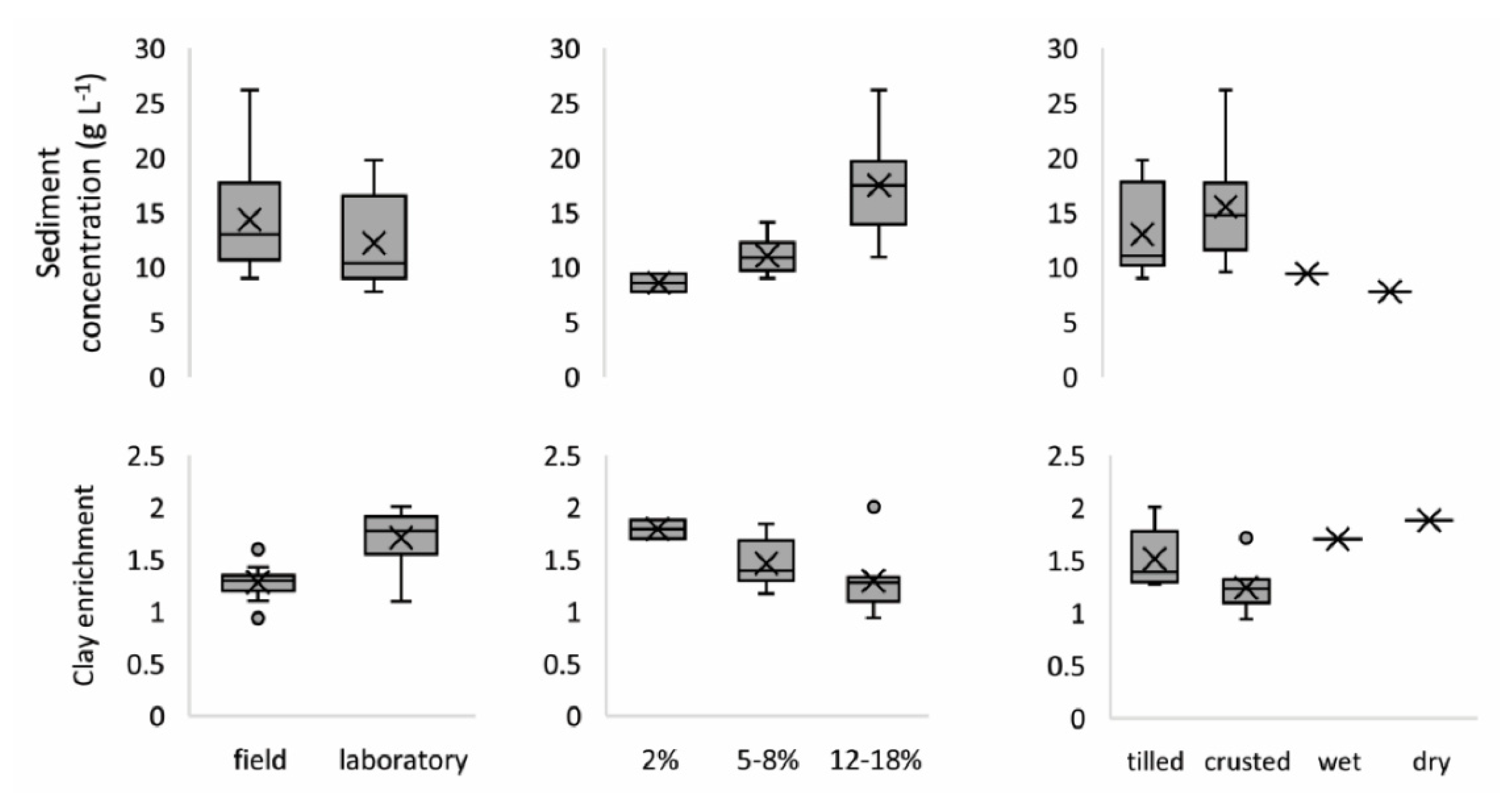
3.2. Variations in Sediment Concentration and Composition

SC values increased and differed significantly (H(18) = 11.075, p = 0.004) with the slope gradient, but were unaffected by the location or surface roughness ( p 0.129 ; Figure 5). On the gentler (2–8%) slopes, SC values of 9–14 and 8–11 g L−1 were recorded, while on the steep (12–18%) slopes, SC values of 10–26 and 15–20 g L−1 were observed in the field and laboratory, respectively (Table A1).
The lowest SC values of 5.5 and 9.2 g L−1 were measured in the runoff from the experiments with a slope gradient of 2% slope and extremely wet or dry initial moisture contents, respectively. The SC was higher in the field when surfaces were crusted (Table 3).
The difference in PSD between the in situ soil and soil loss was expressed by the CE ratio. As a general result, all soil loss had a CE > 1, except for the highest SC-related rain with the highest runoff ratio (CE = 0.94). Moreover, CEs were significantly higher in the laboratory (U(NField = 12, NLab = 6) = 61, p = 0.018) (Figure 5, Table A1) compared to the field measurements. In contrast, CE did not vary significantly, neither with regards to the slope gradient (H(18) = 5.088, p = 0.079) nor the surface roughness (H(18) = 6.868, p = 0.076).

3.3. Regulating Properties of SC for Various Rainfall Simulations

By analyzing the linear relationships of the response variables, we found that the first two PCs (PC1 and PC2) were able to account for approx. 80% of the total original variance in both the laboratory and field experiments together (Table 4a). After correlating the PC scores with the explanatory variable, we found that the main influencing factors of SC differed between the field and laboratory (Table 4).
The most influential parameters in the first PC for the field measurements were constant runoff/infiltration, constant runoff rate, particle size median of soil loss with a positive load, and ponding period with a negative sign indicating a response opposite to the others (Table 4a). Specifically, if the surface was smooth (short ponding period), the constant runoff rate increased, the flow could transport larger particles/aggregates, and the PSD median also increased. The first PC displayed a strong and significant (p < 0.01) linear relationship with the explanatory variable SC (Table 4b). The variance compressed into the second PC for the field measurements mostly accounted for the rainfall intensity, which had a smaller linear effect on SC (Table 4b). The loadings of slope gradient did not fall within the chosen ±0.7 interval in neither PC, indicating a secondary effect on SC in the field.
As the slope gradient increased in the laboratory experiments, the rainfall intensity, ponding period, and constant runoff rate decreased according to the first PC (Table 4a); however, the two most determining variables (constant runoff/infiltration and particle size median) in the second PC displayed a parallel change (Table 4a). Significant correlations were observed between the PCs and SC; it was exclusively related to the first PC (Table 4b). Thus, while the actual surface state and development acted together as influential processes on SC in the field, the first PC indicated that, in the laboratory, the constant runoff/infiltration and the particle size median of the soil loss were independent of SC.

4. Discussion

In this study, the soil type, high rainfall intensities, and slope gradients were the matching parameters during the experiments, while initial soil moisture content, surface state (crusting and smoothening), and the device used varied.
No differences were found in time to runoff in either the laboratory or the field. This may suggest that the disturbed soil transported in the laboratory yielded comparable infiltration values with that measured in the field, even though the high variance makes the comparability difficult. In contrast, a larger plot size may trigger poorer surface flow connectivity, resulting in higher ponding capacity in the field, as reported by Langhans et al. [52]. The runoff coefficient values demonstrated the impact of the crust on runoff in both locations, as roughness affected the drainage network [53] and a sealed surface inhibited infiltration [54], although, without the measurement of surface roughness and micro-topography, this is just an indication of its veracity. Initial soil moisture content could also affect the initiation of runoff; it begins earlier on a wet surface, as reported by Jin et al. [7]. Gómez and Nearing [55] also observed delayed time to runoff owing to higher surface roughness, but they did not observe differences in the runoff coefficient. This might have been due to the changes in surface connectivity, which could drastically affect the runoff volume even on rough surfaces [56]. Above and beyond these processes, variations in research design (e.g., differences in kinetic energy, splash loss due to a lack of fences in the laboratory) would surely have contributed to the difference.
As the infiltration–runoff equilibrium of the complex system is affected by several properties, it is impossible to provide a clear explanation of the differences. The point is that the method used will impact the results.
One of the main goals of this study was to test the comparability of field and laboratory SC and CE results. Concerning the constant runoff and constant runoff rate measured in this study, we found that the values from the experiments were similar when conducted on similar slope gradients (Figure 3 and Figure 4). However, the research design (border effect in splash erosion (that is, unmeasured soil loss due to the lack of fences) in the laboratory might decrease SC. At the same time, in the present study, the CE was higher in the laboratory (Figure 5). Zemke [57] also demonstrated the enrichment of fine particles in soil loss on small plots under simulated rainfalls. Presumably, this was due to the smaller plot size, in which deposition of the coarse fraction within a plot is inhibited, as also suggested by Jakab et al. [58], or is simply the result of the higher kinetic energy of the applied rainfall. In contrast, the similar CE from tilled and crusted surfaces of the present study was in contrast to the results of high-intensity small plot experiments on silty loams by Ding and Huang [11].
Concerning the overall erosion process, in the field, both the SC and CE influenced the surface properties, as also reported by Koiter et al. [5]. In the laboratory, the velocity of the moving water and its influencing factors (slope and rainfall intensity) were the main variables driving SC, and the available soil particles and amount of water determined the CE. The above difference, however, is an artefact of the different research designs, including, among others, the plot size, the border effect, and the differences in the drop spectra and kinetic energy of the rain. To achieve more precise and detailed results, additional measurements are needed with a greater degree of standardization in the conduct of the experiments (e.g., using the same nozzles in the field and the laboratory). Moreover, given that the above findings are the results of experiments carried out on a single soil, more investigations on other soil types are required before the results can be generalized.

5. Conclusions

Results gained using the two simulators agree with each other and reflect in similar ways on the soil and surface properties. Therefore, both simulators are suitable for calculations concerning the susceptibility of soils to erosion, and their results are comparable. The slope gradient was found to be an effective regulator only in the laboratory. Rainfall intensity was also more effective in the laboratory than in the field simulations. This, then, suggests that soil-related properties had a prominent role in driving sediment concentration in the field, whereas in the laboratory, slope and rainfall intensity were found to be driving factors independent of soil-regulated sediment concentrations. However, these findings are based on a limited number of simulations and investigate only one type of soil, and some may conclude that different rainfall simulators behave differently, resulting in the overestimation of the role of various sub-processes. Thus, the research design of a rainfall simulator may affect the results even though the differences thus evoked seem to be small in magnitude, probably beneath the sampling error caused by natural spatial heterogeneity of the soil. Ideally, in the future, an optimal research design will be to use paired scenarios for various simulation purposes. To do so, many comparative measurements are needed.

Author Contributions

Conceptualization, J.A.S. and G.J.; methodology, J.A.S., B.K. and G.J.; formal analysis, I.G.H.; investigation, C.C., E.D., and B.K.; writing—original draft preparation, J.A.S.; writing—review and editing, Z.S. and G.J. with contribution from I.G.H.; visualization, J.A.S.; supervision, G.J. All authors have read and agreed to the published version of the manuscript.

Funding

This research was funded by the Development and Innovation Fund of Hungary, grant number NKFIH 123953.

Acknowledgments

The authors are grateful to Paul Thatcher and Lyndre Nel for the English language advice.

Conflicts of Interest

The authors declare no conflict of interest. The funders had no role in the design of the study; in the collection, analyses, or interpretation of data; in the writing of the manuscript; or in the decision to publish the results.

Appendix A

Table A1. Measured drop spectrum of the SP-02 rainfall simulator in the field at a pressure of 0.41 KPa using WATOR (Macherey-Nagel) adsorption papers and digital image analysis.
Drop Diameter (mm)<0.50.5–1.01.0–2.02.0–3.03.0–4.04.0–5.0>5.0Total
No. of drops641504224116501981562
Kinetic energy (J m−2 mm−1)0.0060.1011.3965.1246.9186.3285.10224.975
Table A2. Calculation of the final constant runoff (mm h−1) using linear regression on the measured runoff/time dataset. Constant runoff is calculated as the steepness of the function (parameter a in y = ax − b). The number of points gives the quantity of measured data used to fit on.
Experiment IDFitted EquationCoefficient of DeterminationNumber of Points
FG1y = 26.448x − 3.70860.9986
FG2y = 52.78x − 2.69020.9937
FG3y = 33.021x − 2.16060.9997
FG4y = 48.244x − 1.45490.9996
FG5y = 30.171x − 2.8310.9986
FG6y = 48.066x − 2.48280.9995
FS1y = 33.761x − 3.18410.9995
FS2y = 60.976x − 1.49150.9997
FS3y = 29.21x − 1.24050.9996
FS4y = 46.646x − 0.82940.9997
FS5y = 19.737x − 1.22860.9977
FS6y = 44.645x − 1.28340.9996
LG1y = 58.022x − 20.5570.99830
LG2y = 66.651x − 12.4520.99916
LS1y = 44.694x − 11.6950.9949
LS2y = 62.804x − 0.77520.99912
LP1y = 66.917x − 2.14610.9999
LP2y = 75.973x − 25.3590.99910
Table A3. Main properties and calculated parameters of the simulations.
Experiment IDLocationMeasured Rainfall Intensity (mm h−1)Slope Steepness (%)Amount of Rain (mm)Time to Ponding (s)Ponding Duration (s)Time to Runoff (s)Runoff Duration (s)Runoff after the Rain (s)Runoff Ratio (%)Infiltration Ratio (%)Sediment Concentration
(g L−1)
Total Soil Loss (g)Runoff CoefficientFinal Constant Runoff
(mm h−1)
Clay Enrichment in Soil Loss
FG1field56.24716.81774211995785475310.6270.60.3026.41.60
FG2field84.68710.63183654398611623812.6306.20.5352.81.30
FG3field70.19813.5320577761824647539.0222.90.3533.01.35
FG4field86.12810.41112738397319564411.3294.60.5248.21.17
FG5field56.92815.19167389872877534710.0318.10.4530.21.43
FG6field80.44812.40241236519661604014.1418.70.5148.11.30
FS1field66.781816.49482876813208514910.9339.40.3433.81.28
FS2field103.481811.67163349357559594117.9582.50.5361.01.32
FS3field49.891710.53253156704112594119.2555.40.5029.21.28
FS4field63.16178.05102636423120742626.2812.10.7046.60.94
FS5field44.51713.86357601061170445613.4407.10.3819.71.33
FS6field76.691711.1825934491210584217.1537.60.5144.61.10
LG1laboratory118593.689258510101694154495111.2138.50.2558.01.84
LG2laboratory141578.65441845251483047539.6111.00.3266.61.71
LS1laboratory1091263.4039918417167783415919.8189.70.2344.72.01
LS2laboratory1021223.890118420623815.565.90.6062.81.10
LF1laboratory108235.7007272111832762389.492.60.5666.91.70
LF2laboratory134279.803498210161128057437.855.40.2576.01.88

References

  1. García-Ruiz, J.M.; Beguería, S.; Nadal-Romero, E.; González-Hidalgo, J.C.; Lana-Renault, N.; Sanjuán, Y. A meta-analysis of soil erosion rates across the world. Geomorphology 2015, 239, 160–173. [Google Scholar] [CrossRef] [Green Version]
  2. Balacco, G. The interrill erosion for a sandy loam soil. Int. J. Sediment Res. 2013, 28, 329–337. [Google Scholar] [CrossRef]
  3. Vahabi, J.; Nikkami, D. Assessing dominant factors affecting soil erosion using a portable rainfall simulator. Int. J. Sediment Res. 2008, 23, 376–386. [Google Scholar] [CrossRef]
  4. Assouline, S.; Ben-Hur, M. Effects of rainfall intensity and slope gradient on the dynamics of interrill erosion during soil surface sealing. Catena 2006, 66, 211–220. [Google Scholar] [CrossRef]
  5. Koiter, A.J.; Owens, P.N.; Petticrew, E.L.; Lobb, D.A. The role of soil surface properties on the particle size and carbon selectivity of interrill erosion in agricultural landscapes. Catena 2017, 153, 194–206. [Google Scholar] [CrossRef]
  6. Bagarello, V.; Di Stefano, C.; Ferro, V.; Kinnell, P.I.A.; Pampalone, V.; Porto, P.; Todisco, F. Predicting soil loss on moderate slopes using an empirical model for sediment concentration. J. Hydrol. 2011, 400, 267–273. [Google Scholar] [CrossRef]
  7. Jin, K.; Cornelis, W.M.; Gabriels, D.; Schiettecatte, W.; De Neve, S.; Lu, J.; Buysse, T.; Wu, H.; Cai, D.; Jin, J.; et al. Soil management effects on runoff and soil loss from field rainfall simulation. Catena 2008, 75, 191–199. [Google Scholar] [CrossRef]
  8. Shi, P.; Van Oost, K.; Schulin, R. Dynamics of soil fragment size distribution under successive rainfalls and its implication to size-selective sediment transport and deposition. Geoderma 2017, 308, 104–111. [Google Scholar] [CrossRef]
  9. Warrington, D.N.; Mamedov, A.I.; Bhardwaj, A.K.; Levy, G.J. Primary particle size distribution of eroded material affected by degree of aggregate slaking and seal development. Eur. J. Soil Sci. 2009, 60, 84–93. [Google Scholar] [CrossRef]
  10. Asadi, H.; Moussavi, A.; Ghadiri, H.; Rose, C.W. Flow-driven soil erosion processes and the size selectivity of sediment. J. Hydrol. 2011, 406, 73–81. [Google Scholar] [CrossRef] [Green Version]
  11. Ding, W.; Huang, C. Effects of soil surface roughness on interrill erosion processes and sediment particle size distribution. Geomorphology 2017, 295, 801–810. [Google Scholar] [CrossRef]
  12. Kuhn, N.J.; Armstrong, E.K.; Ling, A.C.; Connolly, K.L.; Heckrath, G. Interrill erosion of carbon and phosphorus from conventionally and organically farmed Devon silt soils. Catena 2012, 91, 94–103. [Google Scholar] [CrossRef]
  13. Ouyang, W.; Xu, X.; Hao, Z.; Gao, X. Effects of soil moisture content on upland nitrogen loss. J. Hydrol. 2017, 546, 71–80. [Google Scholar] [CrossRef]
  14. Stroosnijder, L. Measurement of erosion: Is it possible? Catena 2005, 64, 162–173. [Google Scholar] [CrossRef]
  15. Poesen, J. Soil erosion hazard and mitigation in the Euro-Mediterranean region: Do we need more research? Hung. Geogr. Bull. 2015, 64, 293–299. [Google Scholar] [CrossRef] [Green Version]
  16. Iserloh, T.; Ries, J.B.; Arnáez, J.; Boix-Fayos, C.; Butzen, V.; Cerdà, A.; Echeverría, M.T.; Fernández-Gálvez, J.; Fister, W.; Geißler, C.; et al. European small portable rainfall simulators: A comparison of rainfall characteristics. Catena 2013, 110, 100–112. [Google Scholar] [CrossRef] [Green Version]
  17. Defersha, M.B.; Melesse, A.M. Effect of rainfall intensity, slope and antecedent moisture content on sediment concentration and sediment enrichment ratio. Catena 2012, 90, 47–52. [Google Scholar] [CrossRef]
  18. Aksoy, H.; Unal, N.E.; Cokgor, S.; Gedikli, A.; Yoon, J.; Koca, K.; Inci, S.B.; Eris, E. A rainfall simulator for laboratory-scale assessment of rainfall-runoff-sediment transport processes over a two-dimensional flume. Catena 2012, 98, 63–72. [Google Scholar] [CrossRef]
  19. Jakab, G.; Kiss, K.; Szalai, Z.; Zboray, N.; Németh, T.; Madarász, B. Soil Organic Carbon Redistribution by Erosion on Arable Fields. In Soil Carbon; Hartemnik, A.E., McSweeney, K., Eds.; Springer International Publishing: Cham, Switzerland, 2014; pp. 289–296. [Google Scholar] [CrossRef]
  20. Rodrigo Comino, J.; Iserloh, T.; Lassu, T.; Cerdà, A.; Keesstra, S.D.; Prosdocimi, M.; Brings, C.; Marzen, M.; Ramos, M.C.; Senciales, J.M.; et al. Quantitative comparison of initial soil erosion processes and runoff generation in Spanish and German vineyards. Sci. Total Environ. 2016, 565, 1165–1174. [Google Scholar] [CrossRef]
  21. Bryan, R.B.; De-Ploey, J. Comparability of soil erosion measurements with different laboratory rainfall simulators; Comparabilité des mesures d’érosion du sol avec différents simulateurs de pluie de laboratoire. Catena Suppl. 1983, 4, 33–56. [Google Scholar]
  22. Iserloh, T.; Ries, J.B.; Cerdà, A.; Echeverría, M.T.; Fister, W.; Geißler, C.; Kuhn, N.J.; León, F.J.; Peters, P.; Schindewolf, M.; et al. Comparative measurements with seven rainfall simulators on uniform bare fallow land. Z. Geomorphol. Suppl. Issues 2013, 57, 11–26. [Google Scholar] [CrossRef]
  23. Mayerhofer, C.; Meißl, G.; Klebinder, K.; Kohl, B.; Markart, G. Comparison of the results of a small-plot and a large-plot rainfall simulator—Effects of land use and land cover on surface runoff in Alpine catchments. Catena 2017, 156, 184–196. [Google Scholar] [CrossRef]
  24. Sadeghi, S.H.; Harchegani, M.K.; Asadi, H. Variability of particle size distributions of upward/downward splashed materials in different rainfall intensities and Slopes. Geoderma 2017, 290, 100–106. [Google Scholar] [CrossRef]
  25. Chaplot, V.; Le Bissonnais, Y. Field measurements of interrill erosion under different slopes and plot sizes. Earth Surf. Process. Landf. 2000, 25, 145–153. [Google Scholar] [CrossRef]
  26. Birkás, M.; Dekemati, I.; Kende, Z.; Pósa, B. Review of soil tillage history and new challenges in Hungary. Hung. Geogr. Bull. 2017, 66, 55–64. [Google Scholar] [CrossRef] [Green Version]
  27. Szabó, B.; Centeri, C.; Szalai, Z.; Jakab, G.; Szabó, J. Comparison of soil erosion dynamics under extensive and intensive cultivation based on basic soil parameters. Növénytermelés 2015, 64, 23–26. [Google Scholar]
  28. Dövényi, Z. (Ed.) Inventory of Micro Regions in Hungary; MTA Geographical Research Institute: Budapest, Hungary, 2010. [Google Scholar]
  29. Keller, B.; Szabó, J.; Centeri, C.; Jakab, G.; Szalai, Z. Different land-use intensities and their susceptibility to soil erosion. Agrokémia Talajt. Agrokem 2019, 68, 14–23. [Google Scholar] [CrossRef]
  30. Jakab, G.; Madarász, B.; Szabó, J.A.; Tóth, A.; Zacháry, D.; Szalai, Z.; Kertész, Á.; Dyson, J. Infiltration and soil loss changes during the growing season under ploughing and conservation tillage. Sustainability 2017, 9, 1726. [Google Scholar] [CrossRef] [Green Version]
  31. Loch, R.J.; Robotham, B.G.; Zeller, L.; Masterman, N.; Orange, D.N.; Bridge, B.J.; Sheridan, G.; Bourke, J.J. A multi-purpose rainfall simulator for field infiltration and erosion studies. Soil Res. 2001, 39, 599–610. [Google Scholar] [CrossRef]
  32. Zemke, J.J. Set-up and calibration of a portable small scale rainfall simulator for assessing soil erosion processes at interrill scale. Cuad. Investig. Geográfica 2017, 43, 63. [Google Scholar] [CrossRef] [Green Version]
  33. Szabó, J.; Jakab, G.; Szabó, B. Spatial and temporal heterogeneity of runoff and soil loss dynamics under simulated rainfall. Hung. Geogr. Bull. 2015, 64. [Google Scholar] [CrossRef] [Green Version]
  34. Szabó, J.A.; Király, C.; Karlik, M.; Tóth, A.; Szalai, Z.; Jakab, G. Rare earth oxide tracking coupled with 3D soil surface modelling: An opportunity to study small-scale soil redistribution. J. Soils Sediments 2020. [Google Scholar] [CrossRef] [Green Version]
  35. Strauss, P.; Cornejo, J.; Strauss, P.; Pitty, J.; Pfeffer, M.; Mentler, A. Rainfall Simulation for Outdoor Experiments. In Current Research Methods to Assess the Environmental Fate of Pesticides; Jamet, P., Cornejo, J., Eds.; INRA Editions: Versailles, France, 2000; pp. 329–333. [Google Scholar]
  36. Thomaz, E.L.; Pereira, A.A. Misrepresentation of hydro-erosional processes in rainfall simulations using disturbed soil samples. Geomorphology 2017, 286, 27–33. [Google Scholar] [CrossRef] [Green Version]
  37. Wang, Y.; You, W.; Fan, J.; Jin, M.; Wei, X.; Wang, Q. Catena Effects of subsequent rainfall events with di ff erent intensities on runo ff and erosion in a coarse soil. Catena 2018, 170, 100–107. [Google Scholar] [CrossRef]
  38. Zhao, X.; Huang, J.; Gao, X.; Wu, P.; Wang, J. Runoff features of pasture and crop slopes at different rainfall intensities, antecedent moisture contents and gradients on the Chinese Loess Plateau: A solution of rainfall simulation experiments. Catena 2014, 119, 90–96. [Google Scholar] [CrossRef]
  39. Özer, M.; Orhan, M.; Işik, N.S. Effect of particle optical properties on size distribution of soils obtained by laser diffraction. Environ. Eng. Geosci. 2010, 16, 163–173. [Google Scholar] [CrossRef] [Green Version]
  40. Konert, M.; Vandenberghe, J. Comparison of laser grain size analysis with pipette and sieve analysis: A solution fo rthe underestimation of the clay fraction. Sedimentology 1997, 44, 523–535. [Google Scholar] [CrossRef] [Green Version]
  41. Mann, H.; Whitney, D. On a Test of Whether one of Two Random Variables is Stochastically Larger than the Other. Ann. Math. Stat. 1947, 18, 50–60. [Google Scholar] [CrossRef]
  42. Kruskal, W.H.; Wallis, W.A. Use of Ranks in One-Criterion Variance Analysis. J. Am. Stat. Assoc. 1952, 47, 583–621. [Google Scholar] [CrossRef]
  43. Chaplot, V.; Poesen, J. Sediment, soil organic carbon and runoff delivery at various spatial scales. Catena 2012, 88, 46–56. [Google Scholar] [CrossRef]
  44. Cerdan, O.; Le Bissonais, Y.; Souchère, V.; Martin, P.; Lecomte, V. Sediment concentration in interill flow: Interactions between soil surface conditions, vegetation and rainfall. Earth Surf. Process. 2002, 205, 193–205. [Google Scholar] [CrossRef]
  45. Maïga-Yaleu, S.; Guiguemde, I.; Yacouba, H.; Karambiri, H.; Ribolzi, O.; Bary, A.; Ouedraogo, R.; Chaplot, V. Soil crusting impact on soil organic carbon losses by water erosion. Catena 2013, 107, 26–34. [Google Scholar] [CrossRef]
  46. Tabachnick, B.G.; Fidell, L.S. Using Multivariate Statistics, 3rd ed.; Harper-Collins: New York, NY, USA, 1996. [Google Scholar]
  47. Bartlett, M.S. The Effect of Standardization on a χ2 Approximation in Factor Analysis. Biometrika 1951, 38, 337–344. [Google Scholar] [CrossRef]
  48. Hatvani, I.G.; Kovács, J.; Márkus, L.; Clement, A.; Hoffmann, R.; Korponai, J. Assessing the relationship of background factors governing the water quality of an agricultural watershed with changes in catchment property (W-Hungary). J. Hydrol. 2015, 521, 460–469. [Google Scholar] [CrossRef]
  49. Hatvani, I.G.; de Barros, V.D.; Tanos, P.; Kovács, J.; Székely Kovács, I.; Clement, A. Spatiotemporal changes and drivers of trophic status over three decades in the largest shallow lake in Central Europe, Lake Balaton. Ecol. Eng. 2020, 151, 105861. [Google Scholar] [CrossRef]
  50. Cattell, R.B. The Scree Test For The Number Of Factors. Multivar. Behav. Res. 1966, 1, 245–276. [Google Scholar] [CrossRef] [PubMed]
  51. Kaiser, H.F. The Application of Electronic Computers to Factor Analysis. Educ. Psychol. Meas. 1960, 20, 141–151. [Google Scholar] [CrossRef]
  52. Langhans, C.; Diels, J.; Clymans, W.; Van den Putte, A.; Govers, G. Scale effects of runoff generation under reduced and conventional tillage. Catena 2019, 176, 1–13. [Google Scholar] [CrossRef]
  53. Römkens, M.J.M.; Helming, K.; Prasad, S.N. Soil erosion under different rainfall intensities, surface roughness, and soil water regimes. Catena 2002, 46, 103–123. [Google Scholar] [CrossRef]
  54. Di Prima, S.; Concialdi, P.; Lassabatere, L.; Angulo-Jaramillo, R.; Pirastru, M.; Cerdà, A.; Keesstra, S. Laboratory testing of Beerkan infiltration experiments for assessing the role of soil sealing on water infiltration. Catena 2018, 167, 373–384. [Google Scholar] [CrossRef]
  55. Gómez, J.A.; Nearing, M.A. Runoff and sediment losses from rough and smooth soil surfaces in a laboratory experiment. Catena 2005, 59, 253–266. [Google Scholar] [CrossRef]
  56. Antoine, M.; Javaux, M.; Bielders, C. What indicators can capture runoff-relevant connectivity properties of the micro-topography at the plot scale? Adv. Water Resour. 2009, 32, 1297–1310. [Google Scholar] [CrossRef]
  57. Zemke, J.J. Runoff and soil erosion assessment on forest roads using a small scale rainfall simulator. Hydrology 2016, 3, 25. [Google Scholar] [CrossRef] [Green Version]
  58. Jakab, G.; Németh, T.; Csepinszky, B.; Madarász, B.; Szalai, Z.; Kertész, A. The influence of short term soil sealing and crusting on hydrology and erosion at balaton uplands, hungary. Carpathian J. Earth Environ. Sci. 2013, 8, 147–155. [Google Scholar]
Publisher’s Note: MDPI stays neutral with regard to jurisdictional claims in published maps and institutional affiliations.
Figure 1. Location of the field experiment and the collection of soil samples for the laboratory simulations in Hungary (Europe) at Gerézdpuszta settlement in Somogy county (area highlighted grey) (a). Field rainfall simulation (b), the topography (c), and the land use (d) of the investigated catena. Black dots indicate the locations of the field rainfall simulation plots.
Water 12 02856 g001
Figure 2. Photographs of the lab (a) and field (c) simulations and their primary parameters ((b,d), respectively) of the simulators used during the study. Marker explanation: (1) nozzle position; (2) triangular collector; (3) irrigated area; (4) plot boundary.
Water 12 02856 g002
Figure 3. Durations of the ponding, runoff, and post-rain runoff periods at the field and laboratory experiments. Asterisks refer to * crusted, ** wet, and *** dry surface conditions. F—field, L—laboratory; P—plain (2% slope); G—gentle slope; S—steep slope; for details, see Table 2.
Water 12 02856 g003
Figure 4. Comparison of the runoff coefficients, constant runoff rates (mm h−1), and time to runoff (s) in accordance with the location, slope gradient, and surface moisture content/roughness. Boxes represent the interquartile interval, the black line in the middle is the median, and the x is the average; the whiskers indicate 1.5 × the interquartile interval. Values outside this are considered outliers.
Water 12 02856 g004
Figure 5. Comparison of the sediment concentration and clay enrichment in relation to the location, slope gradient, and surface properties. The most striking differences were caused by the slope gradient, and the SC increased while the CE decreased with an increasing slope gradient.
Water 12 02856 g005
Table 1. Main properties of the examined topsoil (0–30 cm layer).
pHdwpHKClCaCO3 (%)SOC * (%)Particle Size Distribution (%)
Clay (<8 µ)Silt (8–50 µ)Sand (>50 µ)
Regosol8.107.405.701.2028.9352.8118.27
* Soil organic carbon.
Table 2. Settings of the 18 laboratory and field rainfall simulation experiments. Identification (ID) code fields are as follows: F: field experiment, L: laboratory experiment; G: gentle slope, S: steep slope; P: plain (2% slope). Runs on steep slopes are in italics and runs under seedbed conditions are underlined.
Experiment IDLocationRainfall Intensity (mm h−1)Slope Steepness (%)Amount of Rain (mm)Rainfall Duration (s)No. of Sub-Samples
FG1field plot 1566.716.81107610
FG2field plot 1846.710.6345210
FG3field plot 270813.536959
FG4field plot 286810.4143510
FG5field plot 3567.715.1996110
FG6field plot 3807.712.4055510
FS1field plot 46618.316.4988910
FS2field plot 410318.311.6740610
FS3field plot 54917.210.5376010
FS4field plot 56317.28.0545910
FS5field plot 64417.613.86112110
FS6field plot 67617.611.1852510
LG1laboratory118593.6827048
LG2laboratory141578.65200814
LS1laboratory1091263.40209416
LS2laboratory1021223.8984316
LP1laboratory108235.70119013
LP2laboratory134279.80214413
Table 3. Comparison of sediment concentrations (g L−1) among the different combinations of slope gradients and surface types. LF1 and LF2 were excluded from this comparison as their experimental setups were unique.
SlopeGentleSteep
Sediment concentration (g L−1)
Field tilled9.93 ± 0.814.30 ± 4.2
Field crusted11.01 ± 1.419.69 ± 5.0
Table 4. Principal component loadings of the first two PCs and their explanatory power expressed as a percentage in parentheses (a). Field and laboratory experiments are both included. Influential loadings (loading outside the +/− 0.70 interval) are in italics, and (b) correlation coefficients between the PC scores and the response variable’s data series, significant at α = 0.1, are marked with an asterisk (*).
(a)Principal Component/Response VariablesFieldLaboratory
1st PC (50.49%)2nd PC (27.23%)1st PC (49.55%)2nd PC (32.55%)
Slope gradient (%)0.3510.6940.879−0.063
Constant runoff/infiltration (%)0.7960.290−0.1110.965
Particle size median (µm)0.7480.5670.5020.746
Rain intensity (mm h−1)0.6430.7060.788−0.384
Ponding period (s)0.7600.0310.8100.079
Constant runoff rate (mm h−1)0.849−0.4960.8120.555
(b)Correlation Coefficient/Explanatory Variable
Sediment concentration (SC)0.71 *0.57 *0.89 *−0.27

