1. Introduction
Flooding is one of the most severe and damaging natural hazards. As revealed by the Emergency Events Database (EM-DAT) Center for Research on the Epidemiology of Disasters (CRED) [
1], from 2005 to 2014, floods accounted for 46% of all natural disasters and affected about 85 million people. During the 20th century, floods were the number-one natural disaster in the United States in terms of the number of lives lost and property damage [
2]. As reported by the Federal Emergency Management Agency (FEMA), from 1978 to 2016, the total amount of paid losses for significant flood events was about USD 46.6 billion. Although this may indicate that climate change is responsible for the increase in flood occurrence and damages, this process is primarily intensified by urbanization [
3]. According to the World Urbanization Report [
4], 54% of the world’s population lives in urban areas, and it is projected that ongoing urbanization and population growth will add 2.5 billion people to the urban population by 2050. The world’s urban percentage increased from 43% in 1990 to 54% in 2014, and it is expected to grow to 66% by 2050. In urban watersheds, the scenario of urbanization is that impervious surfaces, including roads, sidewalks, parking lots, airports, buildings, etc., are replacing the natural soil layer and, as a result, reducing infiltration, which leads to a decrease in travel time and the generation of rapid overland flow. This human modification of land use and land cover (LULC) can significantly influence the watershed hydrological conditions and increases the peak discharge and runoff, which affect people’s lives and properties. At the end of the 1960s, researchers began to focus on understanding the effect of intensive deforestation and urbanization on river systems [
5]. The research was carried out to determine the effect of land use/cover change on urban flooding risk [
6,
7,
8,
9,
10]. Saghafian et al. [
9] found that the deterioration of vegetated land cover led to an increase in flood peak and volume.
All of these human developments and related LULC change issues have led to the necessity of reliable flood and hydrological runoff modeling and predictions for advance warning and protection. Du et al. [
11] applied an integrated simulation of land use changes and hydrological processes to investigate the impact of urbanization on the volume of direct runoff. The simulation results indicate that land use change has significantly increased direct runoff over the past two decades. Romero and Ordenes [
12] concluded that the increased impervious areas in rural lands were causing flash floods. Olaide M et al. [
13] used satellite images to determine the LULC change and how it influences urban flooding. The study found that marginal areas and vegetation were converted to residential areas, which increased the total impervious cover and generally increased the peak runoff. Various contributions have applied hydrological models to estimate and evaluate the impact of LULC change on the urban runoff process, flood magnitude, and frequency [
7,
8,
10,
14,
15,
16]. The Hydrologic Engineering Center Hydrologic Modeling System (HEC-HMS) is one of the semi-distributed models that take into account the spatial variation in the watershed parameters to simulate the rainfall-runoff processes of the watershed systems. The model has been widely applied for simulating runoff in flood risk assessment studies—for example, in [
9,
17]. Further, Oleyiblo and Li [
18] indicated that the model accurately simulated the flood volume and peak time and is a powerful tool for flood forecasting. Koneti et al. [
19] applied HEC-HMS for runoff simulation and found that the model better simulated the runoff at the sub-basin scale. Although there have been numerous urban runoff modeling efforts, as exampled above, our review suggests that there was a lack of understanding of the impact of spatial and temporal heterogeneity of urban development processes on runoff model outcomes. At the regional level, there are often “hot spots” and “cool spots” of urban development in both spatial and temporal domains. How sensitive are the urban runoff models, specifically HEC-HMS, in their ability to reflect these variations in urbanization processes, as indicated by the patterning of LULC change? In previous studies, this issue was not fully and adequately addressed.
In the past decade or so, hydrological modeling has been improved with the development of remote sensing, geographic information systems (GIS), and fine-resolution geospatial data, including satellite imagery, digital elevation models (DEM), and radar rainfall data. The accuracy of spatial information is critical for effective landscape and hydrologic modeling [
20,
21,
22], and model outcomes and their interpretation are heavily dependent on the availability of input data at a given scale [
23]. Although the concept of incorporating satellite imagery and other geospatial data into hydrological modeling is not a recent development, the availability of fine spatial resolution data and the development of modeling and computational tools make it possible to obtain more detailed information needed for landscape and flood risk assessment. In this regard, we find that there is a lack of tests of the feasibility and effectiveness of integrating various forms of geospatial data in a unified runoff simulation. Further, our review indicates that the impact of the quality of geospatial data, specifically different spatial resolutions, on the model outcome has not been fully examined in previous studies, particularly in an urban watershed such as our case study area.
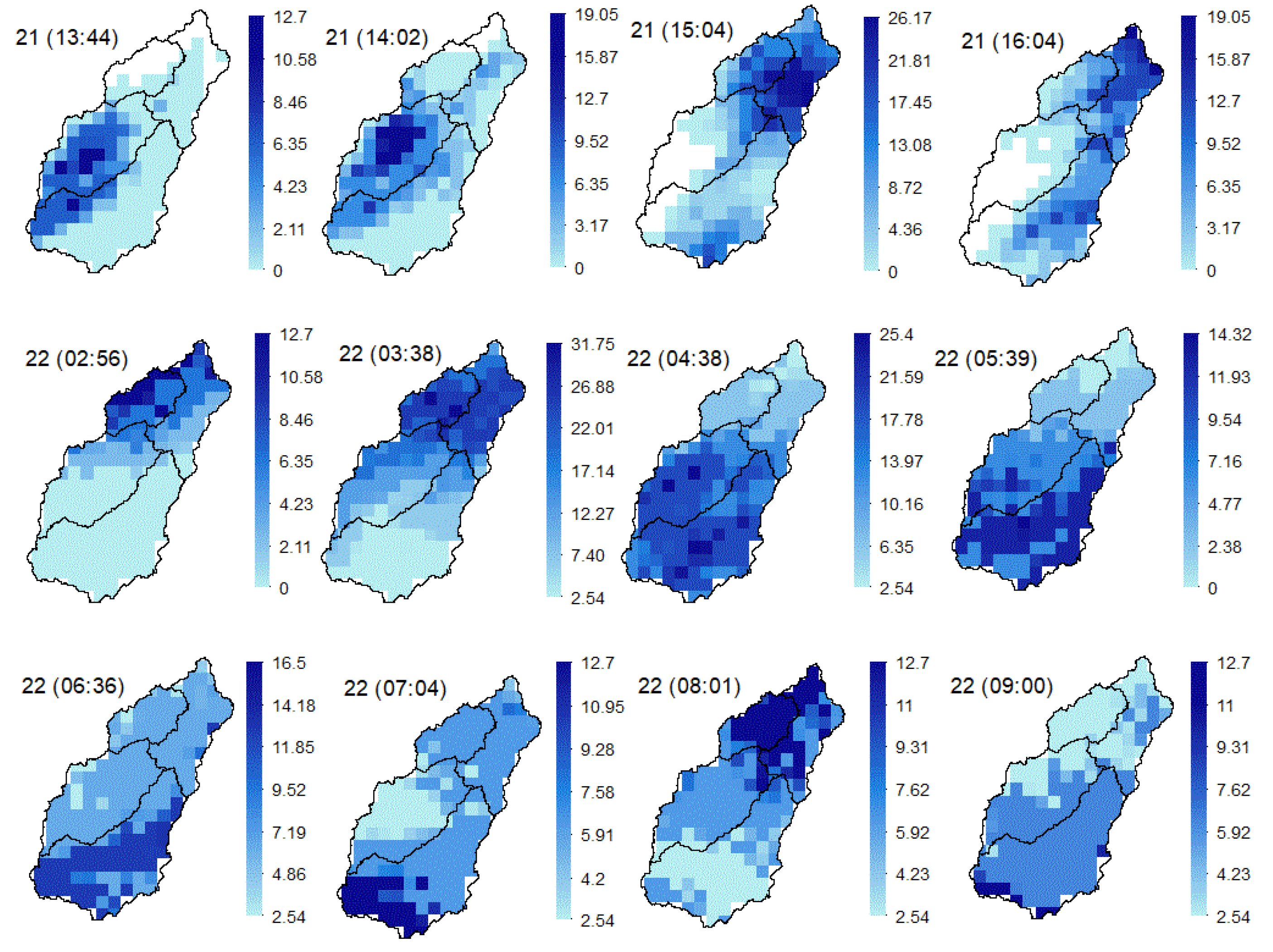
The response of LULC to precipitation varies spatially; thus, spatially distributed rainfall data, such as Next Generation Weather Radar (NEXRAD), are critical in distributed hydrological models, such as HEC-HMS for accurate runoff computation, which requires calculating the mean areal precipitation (MAP) for the watershed. Using this dataset, computing MAP explicitly considers the spatial variability of rainfall compared with ground-based gauge rainfall [
24]. Some previous studies have tested the performance of different NEXRAD precipitation products against the ground-based gauge data in hydrological modeling, and results have shown the superiority of NEXRAD data because of their ability to capture the rainfall spatial variations for better outcomes [
25,
26,
27]. Only a few studies have attempted to couple NEXRAD Level 3 rainfall with the HEC-HMS model for the assessment of LULC change impact on urban flooding. For example, Knebl et al. [
17] used NEXRAD data in HEC-HMS simulations and found that the model tended to overestimate the runoff, and the calibration runs improved the overall results. On the other hand, McCormick [
28] found that the NEXRAD data were effective for utilization with HEC-HMS, and the model produced reasonable results. Given these different findings, a further understanding of this issue is essential.
In summary, all the issues described above raised the research questions: (1) How sensitive are runoff simulation to land use and land cover change patterning? (2) How will input data quality impact the simulation outcome? (3) How effective are integrating and synthesizing various forms of geospatial data for runoff modeling? To address these questions, this study aims to (1) detect LULC changes and assess the impact of the change patterns on the watershed hydrological response (runoff); (2) examine the impact of data quality on simulation outcomes; (3) test the suitability of NEXRAD rainfall data when being used in integration with other geospatial datasets in runoff modeling.
3. Results and Discussion
3.1. LULC Maps, Classification Accuracy, and Change Detection
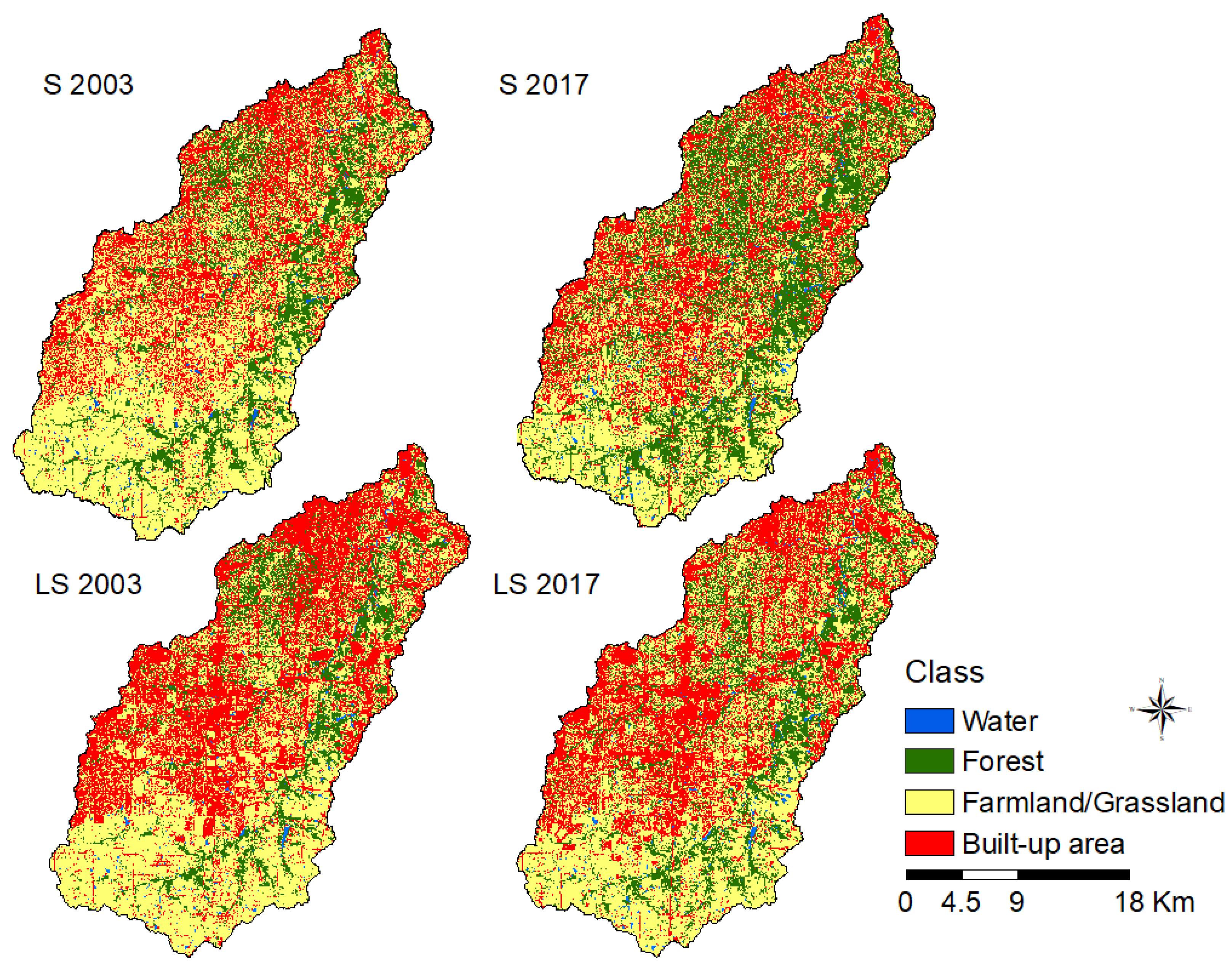
Figure 6 shows the classified LULC maps using SPOT and LANDSAT 2003 images and 2017 images. The use of the higher spatial resolution image (SPOT 6 m), as compared with the lower spatial resolution images (SPOT 20 m), improved the overall classification accuracy.
Table 3 and
Table 4 summarize the classification accuracy assessment results, including producer’s and user’s accuracies for each image. The overall classification accuracy results with SPOT images increased from 85% (2003) to 92% (2017). The overall accuracy results with LANDSAT images are 87.60% for the 2003 image and 84% for the 2017 image. The calculated classification accuracies show satisfactory results for the purpose of this study, in which LULC maps with different resolutions are produced as inputs for the runoff modeling. SPOT and LANDSAT imagery classification results show an increase in water bodies and forestland and a decrease in farmland/grassland. There is a marginal gain in built-up area (
Table 5). As a result, during the study period, farmland and grassland remained the largest land use type, followed by forestland, built-up area, and water bodies.
Change detection statistics were calculated and are shown in
Table 6 and
Table 7. Both classifications reveal an increase in the water class (0.19% from SPOT imagery and 0.15% from LANDSAT imagery). Forestland increased by a higher percentage (11% from SPOT imagery and 4% from LANDSAT imagery). These change patterns might have been caused by efforts to restore the Blue River watershed’s ecosystem, such as a partnership project, called Renew the Blue, that restores riparian forests, upland habitats, and wetlands in the study watershed [
47]. The increase in forestland through forestation activities was mostly at the cost of losing farmland and grassland, according to image classification results. A small decrease in built-up areas might also be associated with the gain in forestland. The built-up area class shows, in SPOT classification results, a decrease of 0.02%, which can be considered as no change, while LANDSAT classification results indicate that the decrease in built-up areas was about 3.67%. These change patterns are consistent with the similar findings of Ji et al.’s [
48] study, which found that, between 1992 and 2010, forestland increased by about 4%; farmland and grassland decreased by about 16%; built-up areas increased by about 10%.
Table 6 and
Table 7 represent the total land cover transformation between 2003 and 2017. For instance, according to SPOT imagery classification results, forestland increased at the expense of farmland/grassland (89.5 km
2) and built-up areas (22.25 km
2). The total loss of farmland and grassland was about 167.61 km
2; 89.5 km
2 was converted to forest or trees, and the rest (76.15 km
2) was converted to built-up areas. In general, forestland has increased the most, whereas the farmland/grassland class has decreased the most. According to LANDSAT imagery classification results, the farmland/grassland class was the larger contributor to the increase in forestland, and both forestland and built-up area classes contributed to the loss of farmland/grassland. The farmland/grassland class was the main land use type in both SPOT and LANDSAT results after 2003. In 2003, the built-up area was the second-largest land use; however, by 2017, forestland became the second-largest land cover in the watershed. Both results show an increase in water bodies, and in general, all classes contributed to this increase. This change detection analysis is essential for understanding the effect of past and current LULC regimes and the effect of LULC change that has been taking place in the watershed and its response to flood events. The study of Ji et al. [
48] indicated that all watersheds in the entire metropolitan area gained about 7% in built-up areas from 1992 to 2010. The above change statistics suggest that our study area (Blue River watershed) had a relatively low rate of urban development and more complex vegetation change patterning during the study period from 2003 to 2017. Naturally, further examination of whether the runoff simulation outcome can reflect such LULC change patterning was carried out, as described in
Section 3.5.
3.2. Watershed Extraction and CN Values
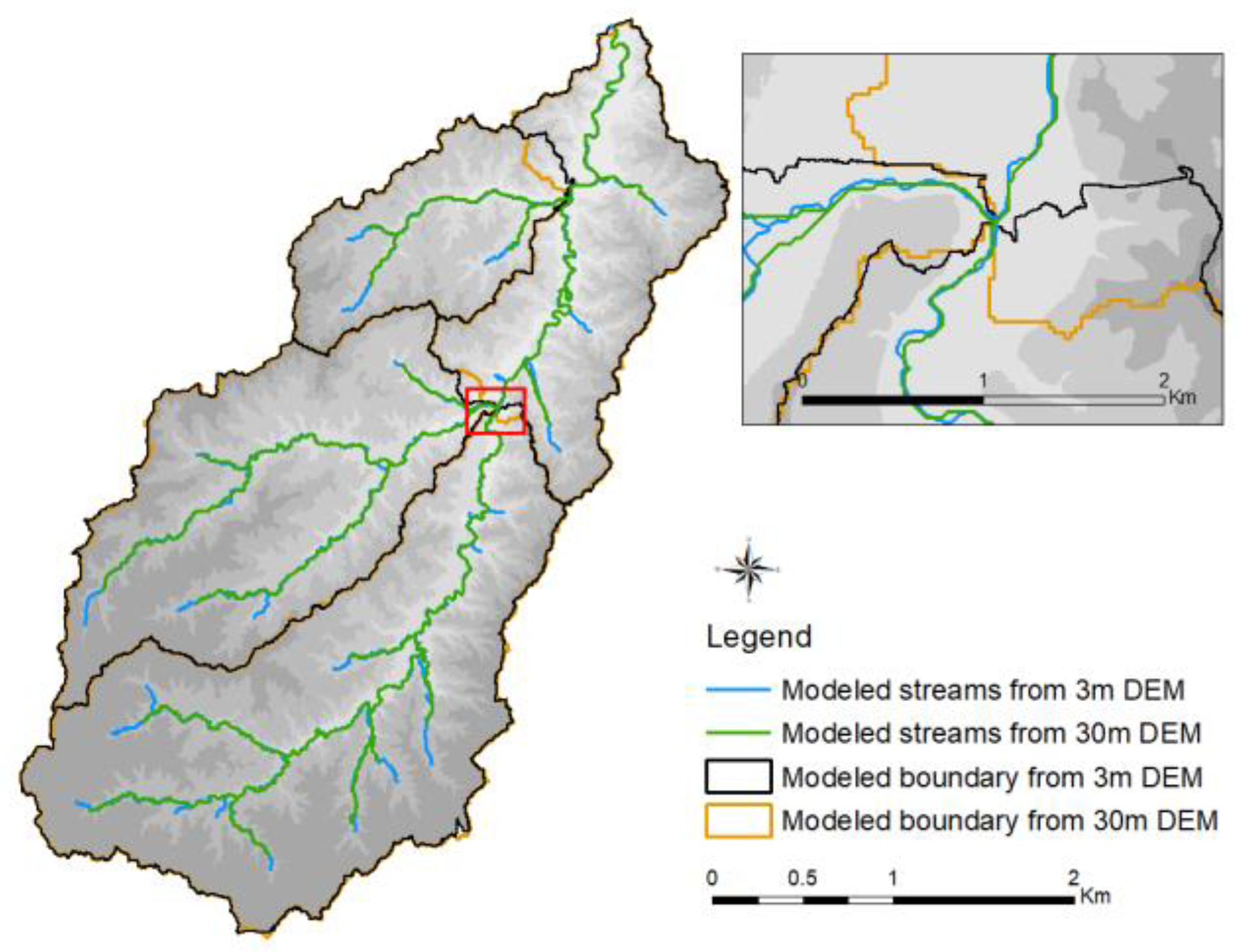
Total stream length and watershed catchment area are often used to measure the level of details extracted from DEMs [
20,
49,
50,
51]. The watershed drainage networks extracted from 3 and 30 m DEMs are shown in
Figure 7. The 3 m DEM represents a total stream length of 230 km and a catchment area of 685.56 km
2, whereas the 30 m DEM represents a total stream length of 178.60 km and a catchment area of 685.59 km
2. The 3 m DEM is sensitive to minor topographic variations, so it captures more details of topographic features. With a vertical resolution of less than 1 m (0.87 m), the 3 m DEM modeled about 51.4 km more streams. Even though the 3 m DEM modeled more stream length, the difference between both results can be considered insignificant. The 3 m DEM produced a more detailed stream network and slightly lower values of basin parameters compared with the 30 m DEM; however, the difference between both DEM results is not significant. Additionally, both DEMs produced the same watershed total area. This outcome agrees with the findings of other studies that have compared the impact of different DEM resolutions on hydrologic and hydraulic modeling results [
51,
52,
53]. Thus, for hydrologic modeling, the use of a moderate-resolution DEM provides reasonable results.
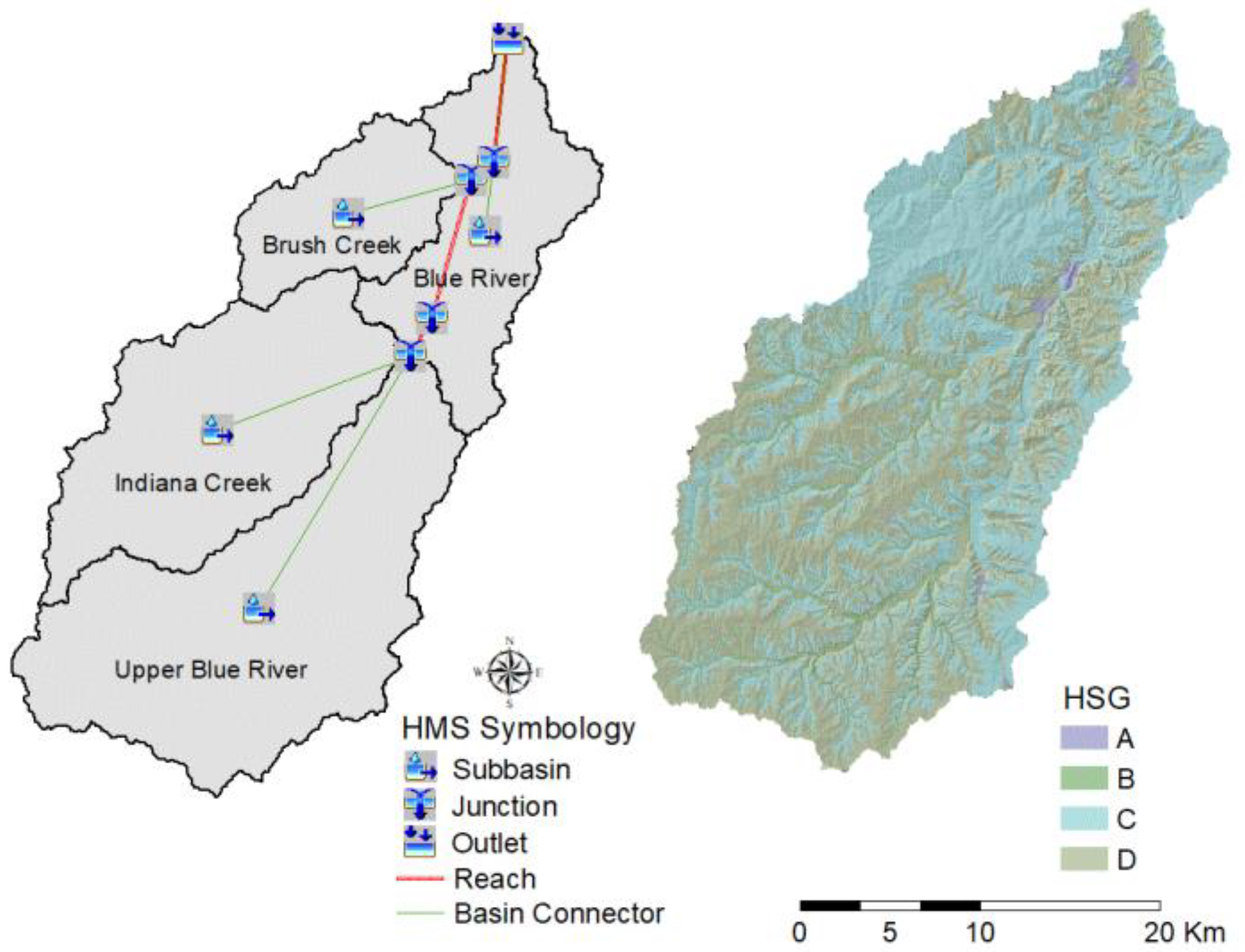
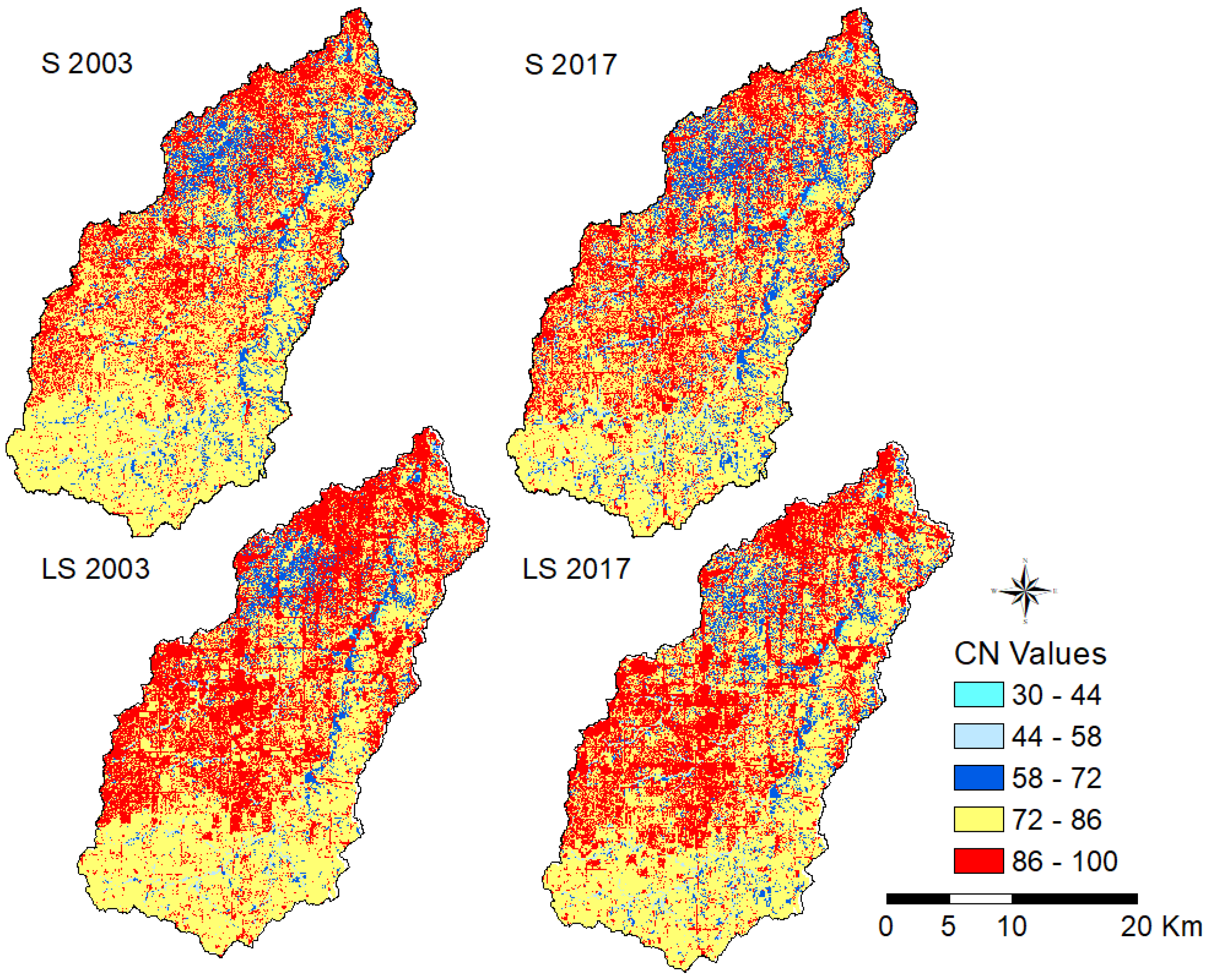
Estimated CN values using SPOT and LANDSAT LULC maps are shown in a color range from 30 to 100 in
Figure 8. Utilizing LULC maps with different spatial resolutions to estimate the CN values produced different results. LANDSAT LULC maps produced slightly higher values. The watershed, in general, has a high CN value even though the built-up area occupies just about 30–35%, and much of the area is vegetated land, which is occupied by farmland, grassland, and forestland. The reason for this is that the majority of the soil covering the watershed is from categories C and D, based on HSG, which usually have low infiltration and high potential runoff.
3.3. NEXRAD Level III Validation
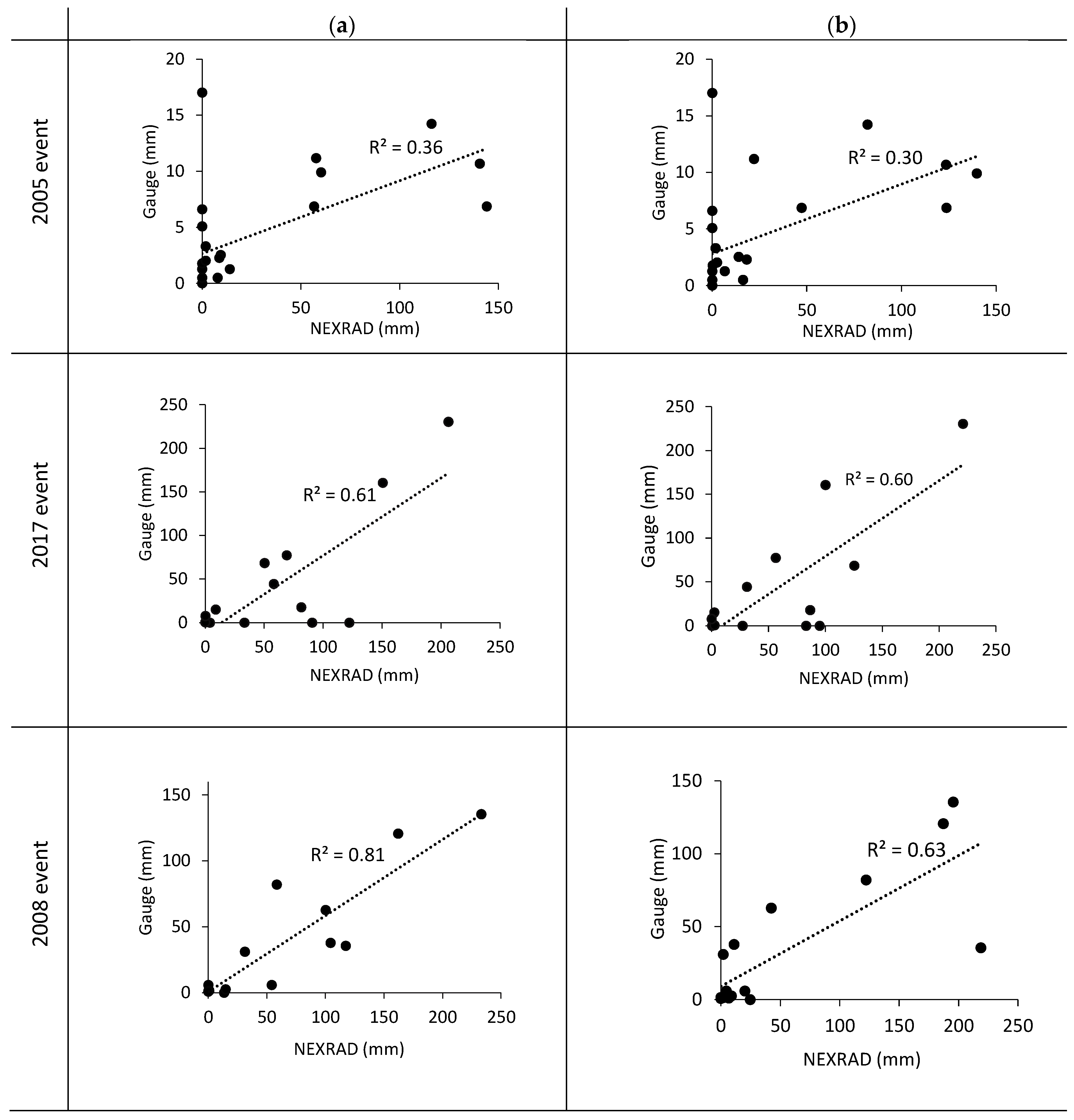
NEXRAD data were validated against gauge rainfall records from three ground-based gauges that were only available for Upper Blue River and Indiana Creek sub-watersheds. Scatter plots in
Figure 9 show a significant correlation between NEXRAD and gauge precipitation data for 2008 (R
2 = 0.8) and 2017 events (R
2 = 0.6), while there is a less significant correlation for the 2005 event (R
2 = 0.30). The Upper Blue River sub-watershed data for the 2008 event display the highest correlation, with an R
2 value of 0.8. In contrast, for the 2005 event, both Upper Blue River and Indiana Creek sub-watersheds show the lowest correlation (R
2 = 0.3). There were some missing data in the gauge records for this event, which affected the correlation results. Validation outcomes of NEXRAD and gauge precipitation usually do not reveal a good relationship because of the possible errors in both of them [
26,
54,
55].
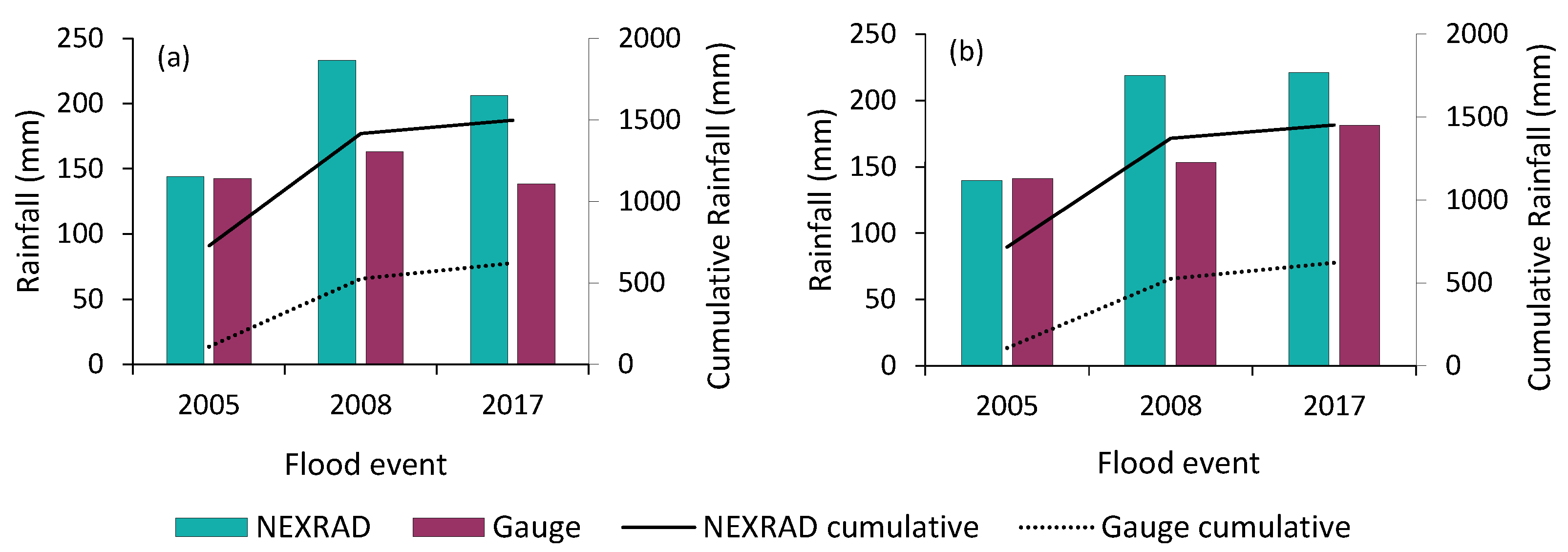
Figure 10 compares the total precipitation of NEXRAD with gauge data. NEXRAD precipitation amounts were overestimated for two flood events compared with gauge rainfall. There is no difference between gauge and NEXRAD rainfall data for 2005 event for both sub-watersheds; however, it is about 0.4 percent for the 2008 event. For the 2017 event, the difference is about 0.2 percent for Indiana Creek and 0.5 percent for Upper Blue River sub-watersheds. The overestimation is probably a result of area (radar grid cell) and point (gauge) errors [
54]. On the other hand, the gauge precipitation might be underestimated due to issues with gauge funnels, which might have been temporarily blocked by grass, bird debris, or other objects, and as a result, the precipitation could be missing or delayed and underestimated [
55].
3.4. Model Calibration and Validation
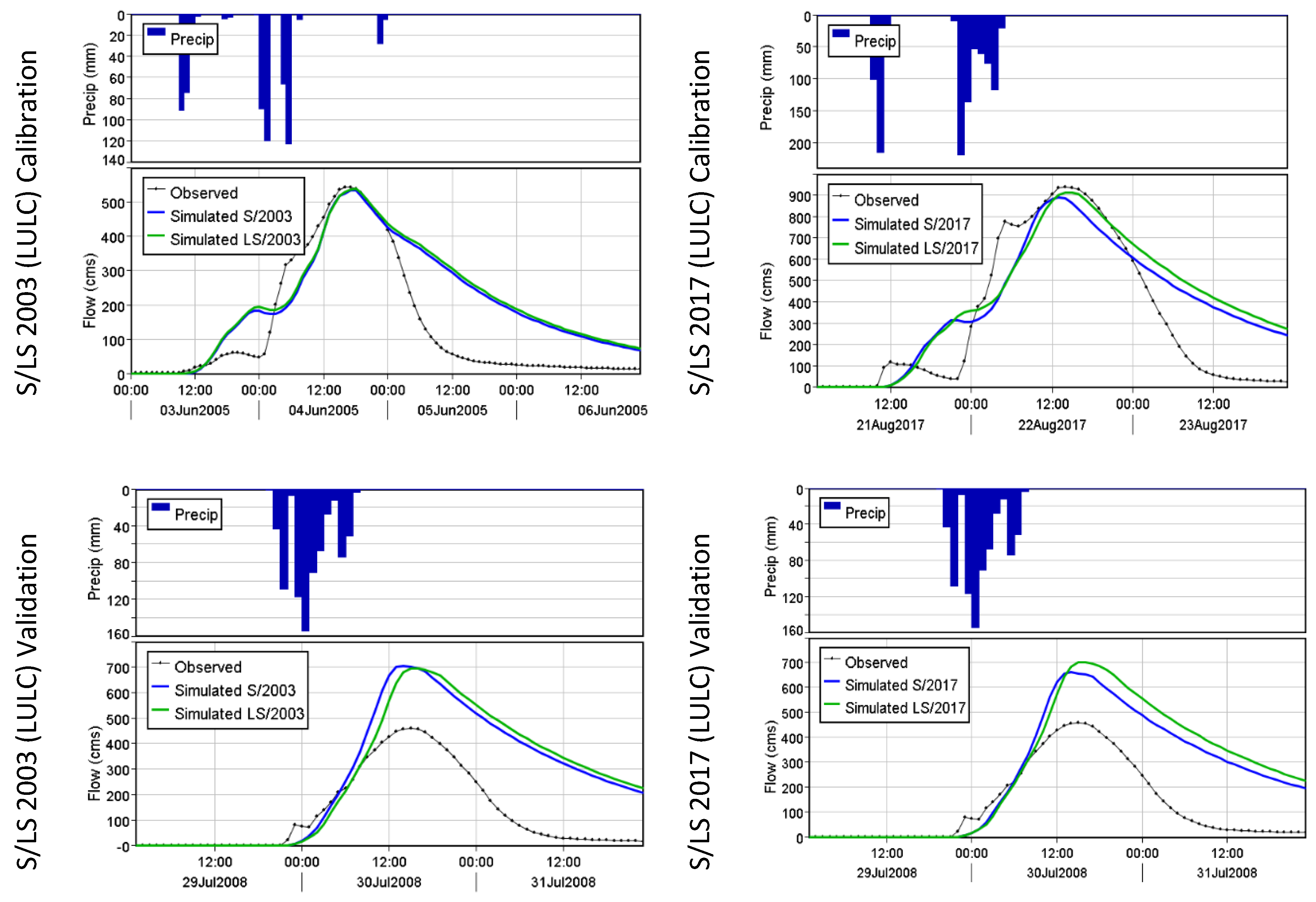
The preliminary simulated runoff hydrographs show a reasonable overall fit with observed data for the watershed. Although the runoff was overestimated in the validation results, the calibration attempts provided better results. Calibration and validation results at the Blue River watershed outlet are shown in
Figure 11.
Model calibration is the derivation of a set of model parameter values that produces the best fit to the observed data; on the other hand, the validation process is running the model for different events without changing the parameters. Calibrated models of 2005 and 2017 events provide better simulation results compared to the 2008 validation models (uncalibrated). There is almost no difference between the observed and calibrated amounts of peak discharge, whereas there is a 0.16 to 0.35 percent difference in direct runoff volume. Validation models provide relatively satisfactory results, although the peak discharge and runoff might be overestimated due to the precipitation amount overestimation in the NEXDAD data. The difference between observed and simulated peak discharge is about 0.36 percent, and direct runoff 0.5 percent. Better estimation for the rainfall amount in NEXRAD data could mitigate the runoff volume and simulate the peak discharge more accurately.
At a sub-watershed level, the model tended to overestimate the runoff for some sub-watersheds, but for the rest of the sub-watersheds, the model more accurately estimated the runoff. Compared with the observed data, the calibrated hydrographs indicate relatively good performance. The difference in statistical results between all models with different data input resolutions and LULC conditions is not significant. All models simulated the runoff in a similar fashion. For instance, the results for the model with lower resolution and 2003 LULC data are E = 0.6, EPBIAS 60%, and RMSE Std Dev = 0.6, and the results for the model with higher resolution and 2017 LULC data are E = 0.7, EPBIAS = 32%, and RMSE Std Dev = 0.5. Thus, using moderate-resolution data (e.g., 30 m) for modeling can still provide satisfactory simulation outcomes. The validation hydrographs of the 2008 event might have been overestimated due to the overestimation of the rainfall in the NEXRAD data. All validation models performed similarly. For example, the results for the model with lower resolution and 2003 LULC data are E = −0.9, EPBIAS 121%, and RMSE Std Dev = 1.4, and the results for the model with higher resolution and 2017 LULC are E = −0.7, EPBIAS = 120%, and RMSE Std Dev = 1.3.
3.5. Impact of LULC Change and Data Quality on Runoff
Using CN values estimated from 2003 (20 and 30 m) LULC maps and basin parameters extracted from 3 and 30 m DEMs, models 1 and 2, simulated with the 2005 event produced similar runoff hydrograph results. With CN values estimated from 2017 (6 and 30 m) LULC maps and basin parameters extracted from 3 m and 30 m DEMs, respectively, models 1.2 and 2.2 simulated with the 2017 event produced close runoff hydrograph results as well. In addition, running models 1 and 2 with the 2017 event and models 1.2 and 2.2 with the 2005 event generated closer results. In other words, all models, when simulating with the corresponding flood events, generated similar runoff hydrographs. For instance, as shown in
Table 8, when simulating the 2005 event under the 2003 LULC condition (Model 1), the results show watershed discharges of 19,217.3 (cms), and under the 2017 LULC condition (Model 1.2), discharges of 19,201.9 (cms) are observed. There is almost no difference between the two discharge amounts. This insignificant variance demonstrates that the simulation reflects outcomes that are consistent with the LULC change patterns in the study area and period. As discussed before, the built-up area in the watershed did not change notably during the study period, while the increase in forestland was offset by decreased farmland/grassland.
Comparing the results of model 1.2, which uses higher spatial resolution data, with model 2.2, which uses lower resolution data, reveals that for each flood event all simulated values are close. For instance, in model 1.2 (uses 6 m LULC and 3 m DEM data), the simulated peak discharge is 33,103.3 cms for the 2017 event, while simulation with model 2.2 (with 30 m LULC and DEM data) results in a peak discharge of 33,295.7 cms. This also shows consistency with the low variation in the CN value and DEM processing outputs derived from different spatial resolution data, which led to similar simulation outputs and performance statistics. In addition, the HEC-HMS model is a generalized model system and applies mathematical models to represent the watershed flow; hence, small differences between derived inputs from 3 and 30 m DEMs or 6 and 30 m images are not enough to notably affect the model outputs. In previous studies, the impact of spatial and temporal heterogeneity of urban development processes on runoff model outcomes was not fully and adequately addressed, particularly in an urban watershed, such as in our case study area. There is a lack of understanding of the impact of different spatial resolutions on the model outcome and the suitability of coupling NEXRAD rainfall with the HEC-HMS model to assess LULC change impact on urban flooding. Our study attempts to further address this issue. In our 14-year study period, we found that the LULC in the Blue River watershed did not significantly change. Since 2003, the buildup area occupied about 1/3 of the watershed, and the majority of the area is vegetated land (forestland, farmland, and grassland). This less dynamic regime of the LULC in the watershed led to similar responses to precipitation and storm events. For runoff simulation applications, it is useful to utilize the standard available data resolution (e.g., 30 m) for satellite images to generate LULC data and CN values, or for DEMs to extract watershed parameters, which may cost less compared with data with higher spatial resolution. As LULC, NEXRAD data vary spatially, which provides a more accurate representation of the rainfall over each area compared with the ground-based gauge data that represent the rainfall amount only in the location area. In our case study, the use of (4 km) NEXRAD precipitation data for the simulation provides reasonably accurate runoff hydrographs. Using the dataset may contribute to runoff overestimation or underestimation due to the uncertainty and error that is usually associated with radar precipitation. At a sub-watershed scale, we found that using HEC-HMS, NEXRAD data can represent the rainfall amount and simulate the runoff for small sub-watersheds more accurately than large ones. Tests of other types of NEXRAD Level III precipitation data, such as the products of “dual-pol,” which clearly identify and detect rainfall, might reduce rainfall overestimation and provide better results.
4. Conclusions
In this study, urban runoff was simulated in an urban watershed that has diverse LULC and development activities, and its streams tend to be frequently flooded. The study aims to understand how LULC change patterning and the quality of input geospatial data affect the simulation outcomes as well as examine the effectiveness of NEXRAD rainfall data in such modeling settings. The study results reveal that the simulation with the HEC-HMS model sensitively responds to the spatial and temporal patterning of LULC dynamics indicated by the change rate of imperious surfaces and vegetated land-use processes. Specifically, the simulation outcomes reflect the slow-down period of urban development and associated ecological restoration efforts in the case study watershed during the study period. The study indicates that the developed simulation approach can better tolerate small variations in derived input parameters, such as CN values, watershed boundaries, parameters, and stream networks, suggesting that input data with a moderate spatial resolution (e.g., 30 m) are suitable for urban runoff simulation at a watershed scale. Further, this study illustrates that, in such modeling, applying spatially distributed precipitation data, such as the one-hour NEXRAD Level III data, provide reliable and satisfactory outcomes after calibration efforts, particularly in hydrograph shape, peak discharge amounts, and time. In addition, the rainfall amount overestimation in NEXRAD data results in higher peak discharge and runoff volume as compared with observed data. Finally, the study proves the feasibility and effectiveness of incorporating satellite imagery-based LULC maps with related geospatial data, including DEM and distributed radar precipitation, in hydrological simulation to assess the watershed’s hydrological response to flooding events.


