Lake Evolution, Hydrodynamic Outburst Flood Modeling and Sensitivity Analysis in the Central Himalaya: A Case Study


Abstract
1. Introduction
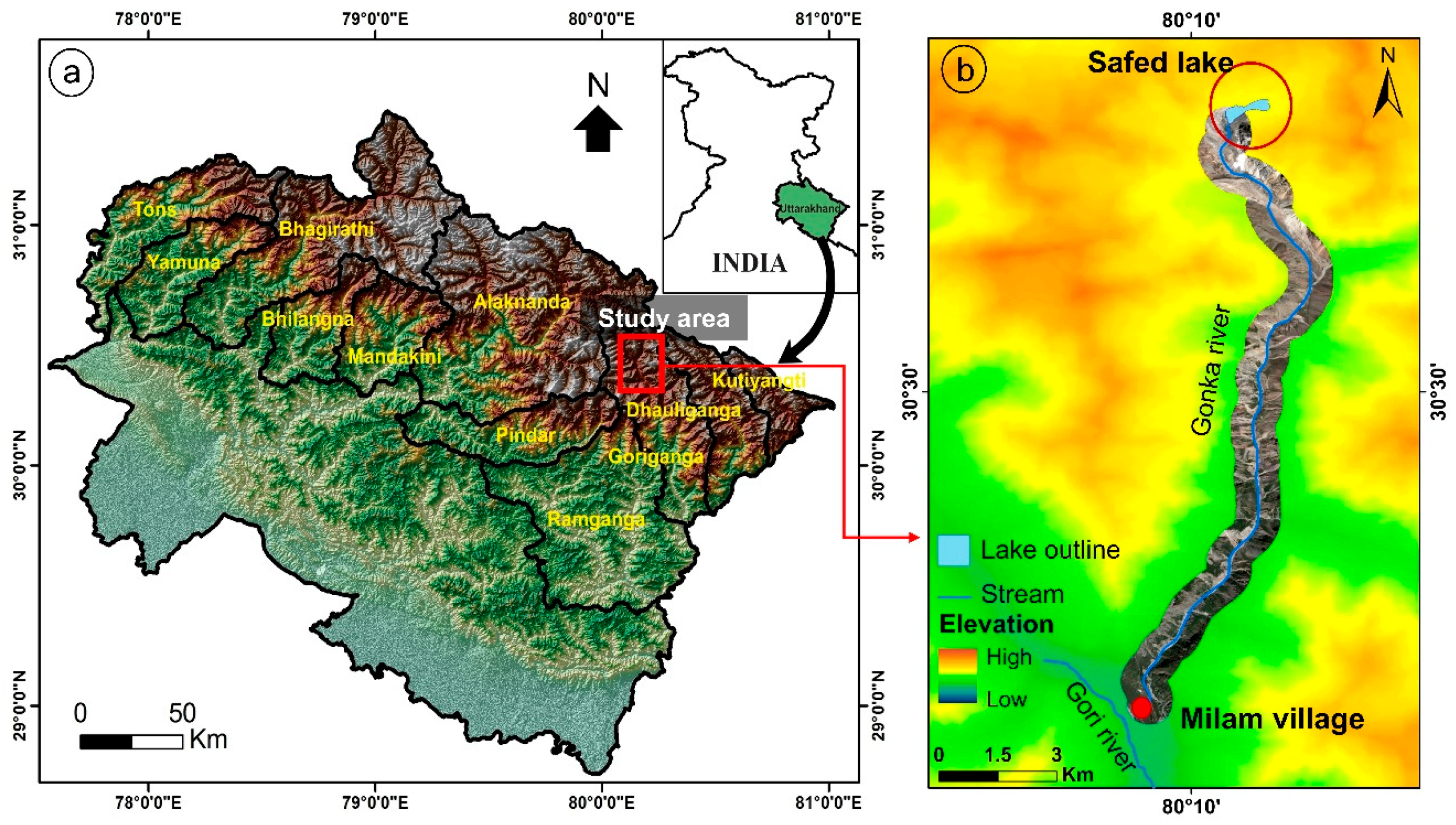
2. Study Area
3. Data and Methods
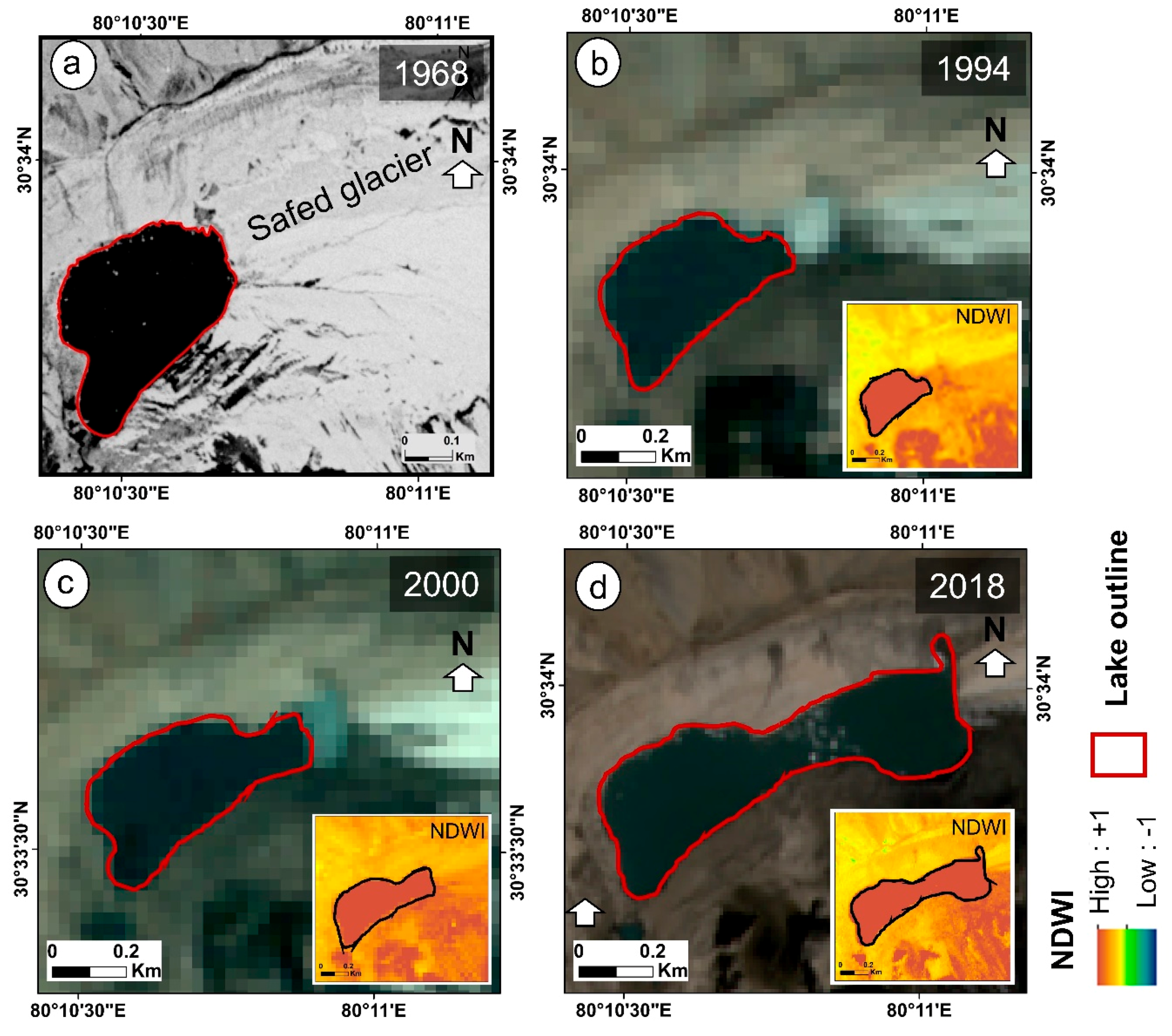
3.1. Remotely Sensed Data and the Growth Assessment of Safed Lake
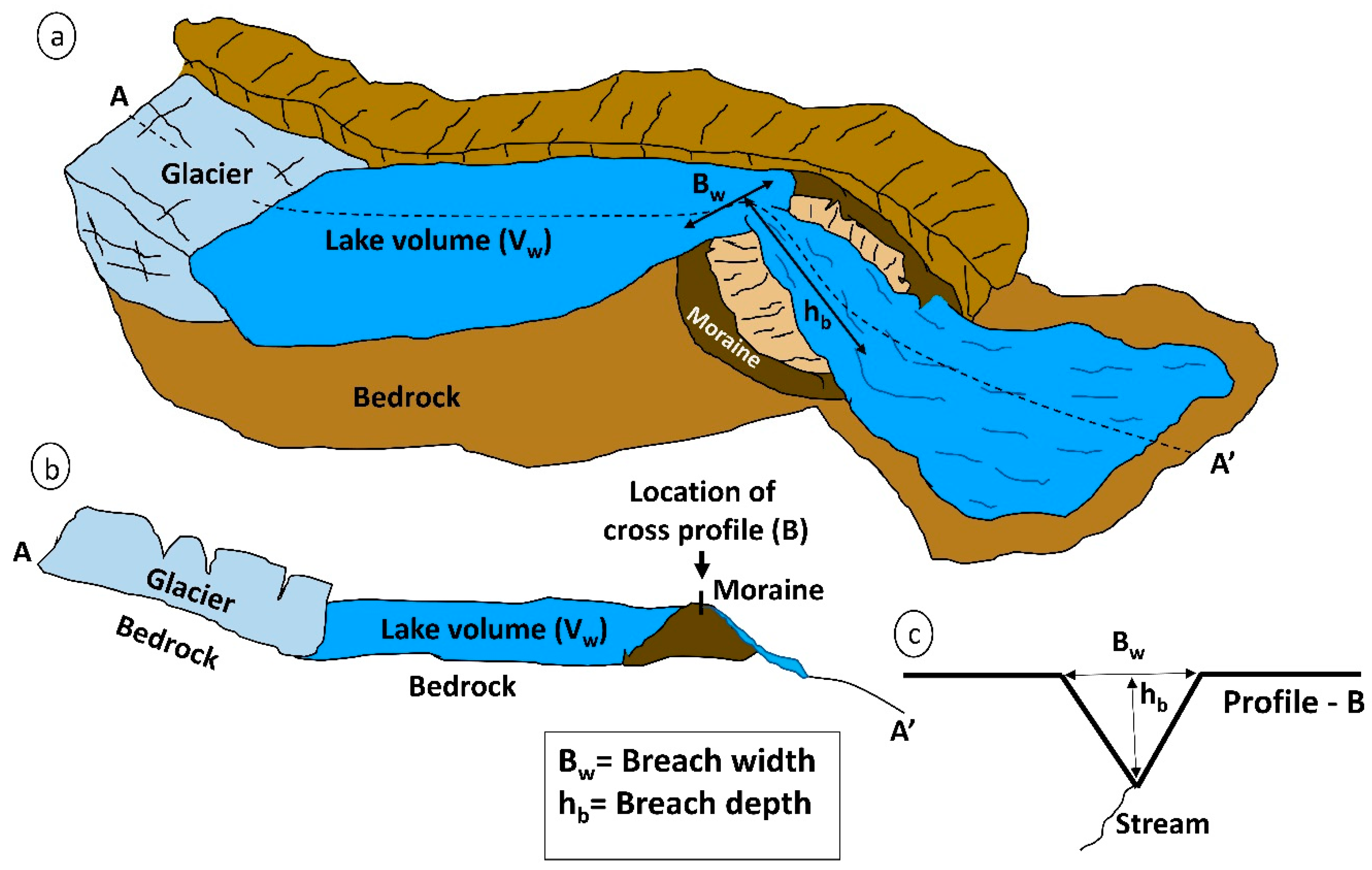
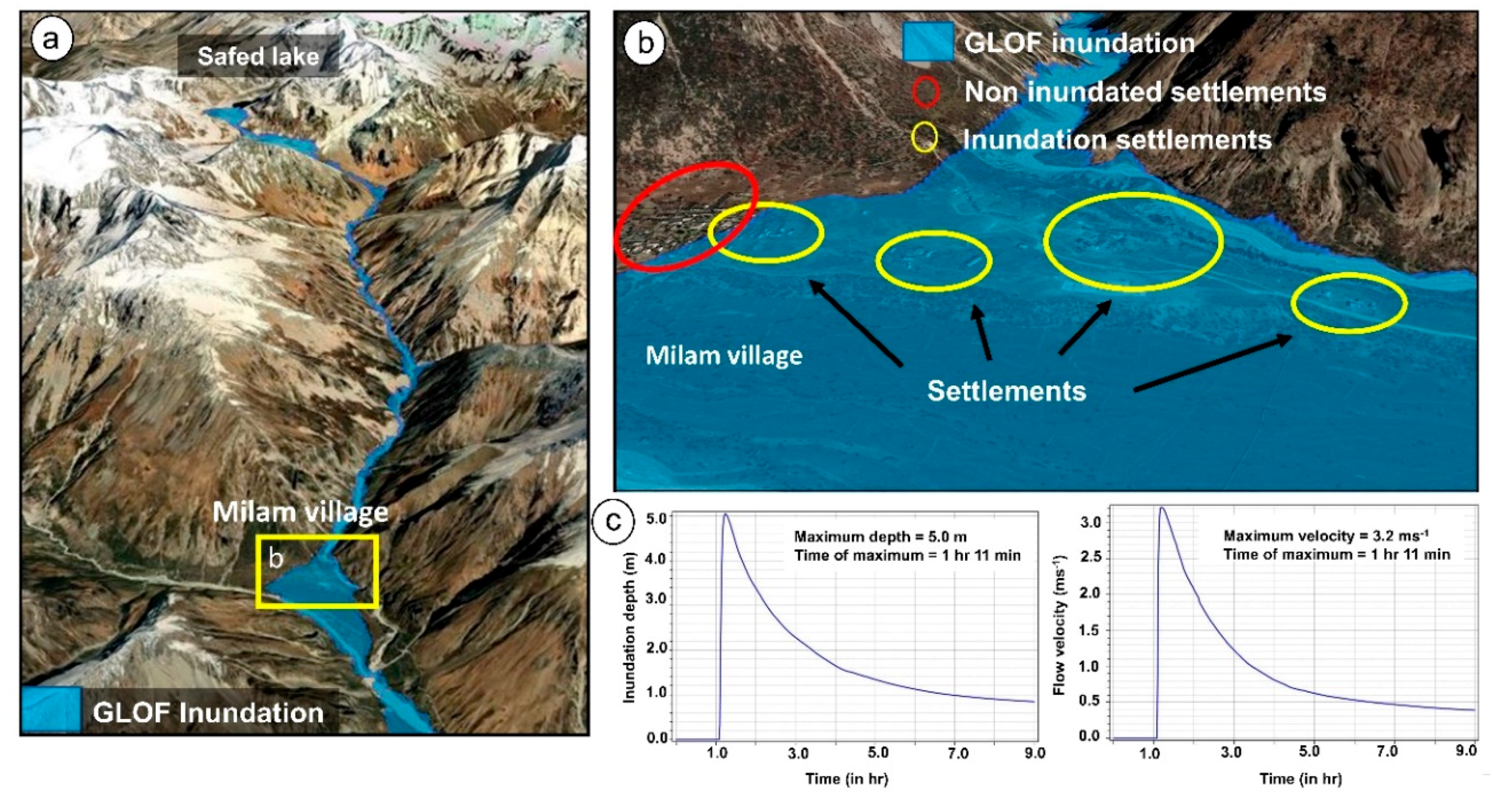
3.2. Hazard Assessment of Safed Lake
3.3. Sensitivity Analysis
3.3.1. Model Sensitivity to Input Parameters
3.3.2. Sensitivity to Channel Characteristics and DEM Used
4. Results
4.1. Growth of Safed Lake
4.2. Hazard Assessment of Safed Lake
4.3. Sensitivity Analysis
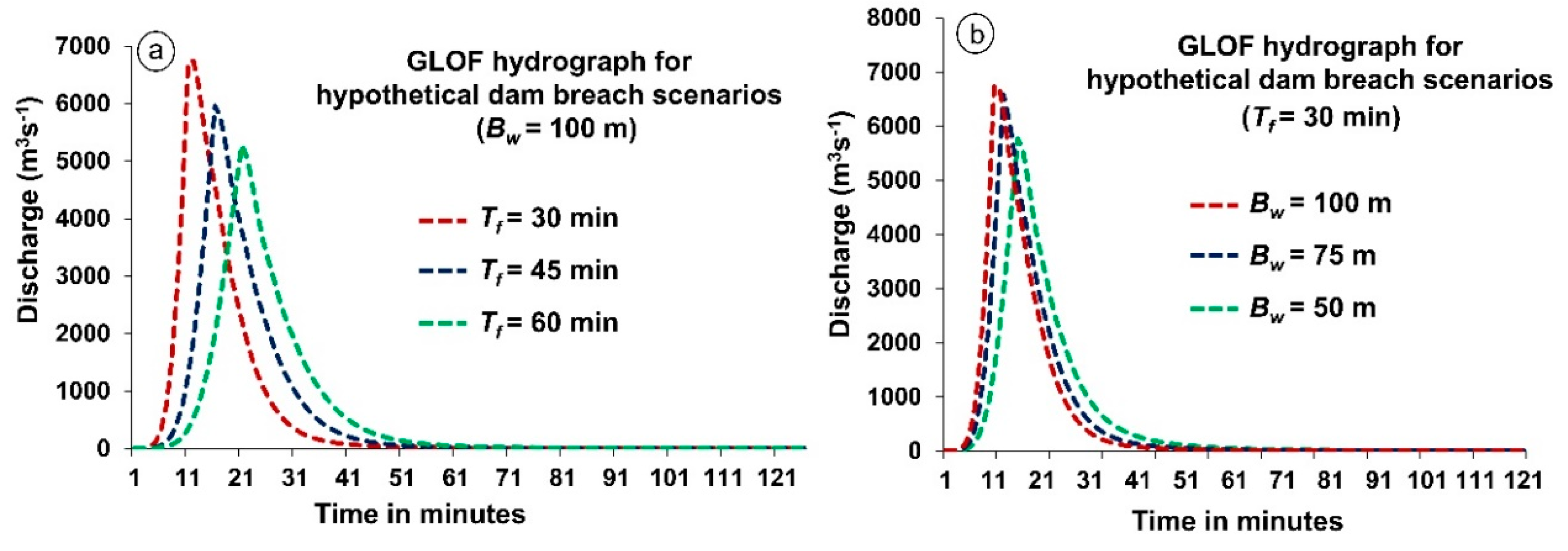
4.3.1. Model Sensitivity to Input Parameters
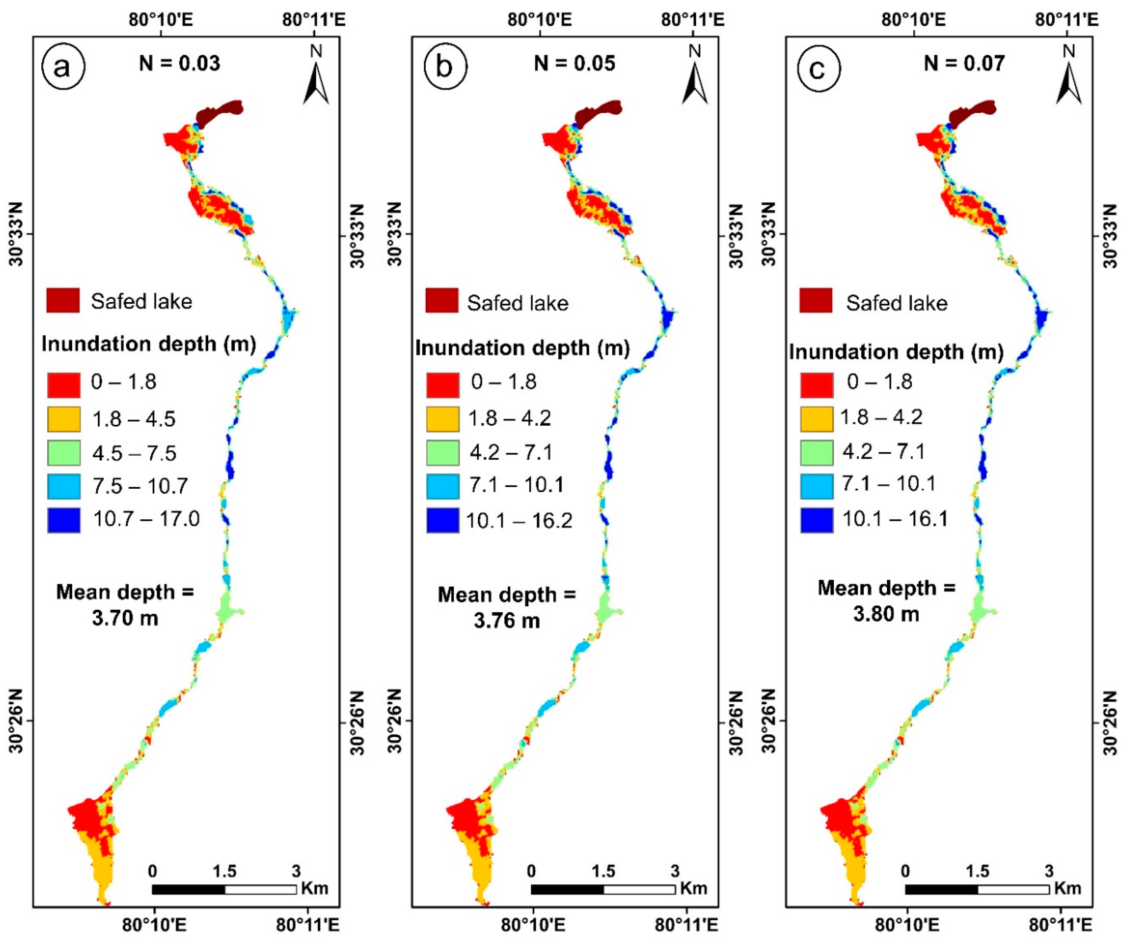
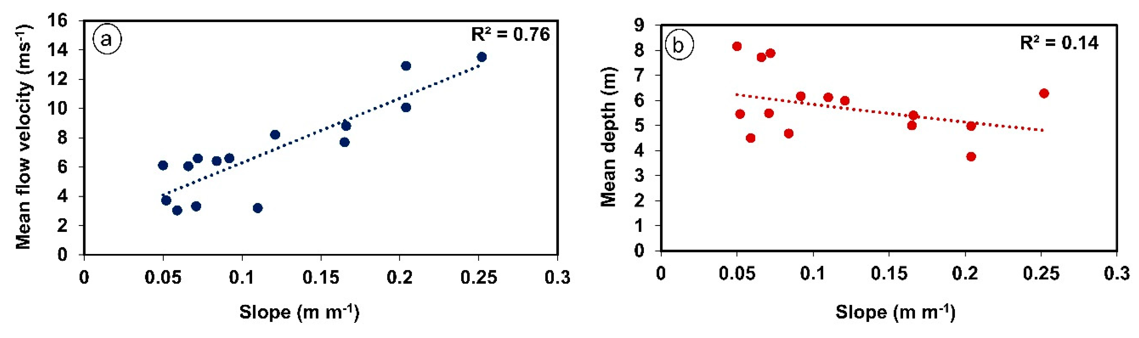
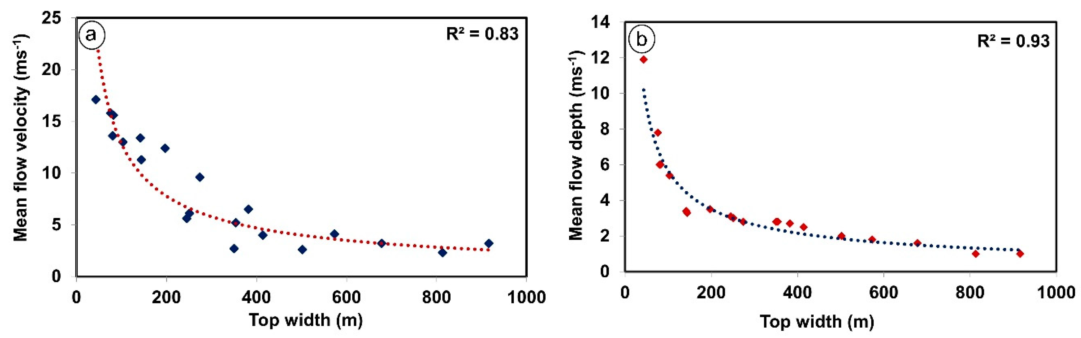
4.3.2. Sensitivity to Channel Characteristics
5. Discussion
6. Conclusions
Author Contributions
Funding
Acknowledgments
Conflicts of Interest
References
- Bolch, T.; Kulkarni, A.; Kääb, A.; Huggel, C.; Paul, F.; Cogley, J.G.; Frey, H.; Kargel, J.S.; Fujita, K.; Scheel, M.; et al. The state and fate of Himalayan glaciers. Science 2012, 336, 310–314. [Google Scholar] [CrossRef] [PubMed]
- Nie, Y.; Sheng, Y.W.; Liu, Q.; Liu, L.S.; Zhang, Y.L.; Song, C.Q. A regional-scale assessment of Himalayan glacial lake changes using satellite observations from 1990 to 2015. Remote Sens. Environ. 2017, 189, 1–13. [Google Scholar] [CrossRef]
- Richardson, S.D.; Reynods, J.M. An overview of glacial hazards in the Himalayas. Quat. Int. 2000, 65, 31–47. [Google Scholar] [CrossRef]
- Veh, G.; Korup, O.; von Sprecht, S.; Roessner, S.; Walz, A. Unchanged frequency of moraine-dammed glacial lake outburst floods in the Himalaya. Nature Clim. Chang. 2019, 9, 379. [Google Scholar] [CrossRef]
- Harrison, S.; Kargel, J.S.; Huggel, C.; Reynolds, J.; Shugar, D.H.; Betts, R.A.; Emmer, A.; Glasser, N.; Haritashya, U.K.; Klimeš, J.; et al. Climate change and the global pattern of moraine-dammed glacial lake outburst floods. Cryosphere 2018, 12, 1195–1209. [Google Scholar] [CrossRef]
- Emmer, A. GLOFs in the WOS: Bibliometrics, geographies and global trends of research on glacial lake outburst floods (Web of Science, 1979–2016). Natural Hazards Earth Syst. Sci. 2018, 18, 813–827. [Google Scholar] [CrossRef]
- Allen, S.K.; Rastner, P.; Arora, M.; Huggel, C.; Stoffel, M. Lake outburst and debris flow disaster at Kedarnath, June 2013: Hydrometeorological triggering and topographic predisposition. Landslides 2016, 13, 1479–1491. [Google Scholar] [CrossRef]
- Carrivick, J.L.; Tweed, F.S. A global assessment of the societal impacts of glacier outburst floods. Glob. Planet. Chang. 2016, 144, 1–16. [Google Scholar] [CrossRef]
- Worni, R.; Huggel, C.; Stoffel, M. Glacial lakes in the Indian Himalayas—From an area-wide glacial lake inventory to on-site and modeling based risk assessment of critical glacial lakes. Sci. Total Environ. 2013, 468, S71–S84. [Google Scholar] [CrossRef]
- Allen, S.K.; Linsbauer, A.; Radhawa, S.S.; Huggel, C.; Rana, P.; Kumari, A. Glacial lake outburst flood risk in Himachal Pradesh, India: An integrative and anticipatory approach considering current and future threats. Nat. Hazards 2016, 84, 1741–1763. [Google Scholar] [CrossRef]
- Raj, K.B.G.; Remya, S.N.; Kumar, K.V. Remote sensing-based hazard assessment of glacial lakes in Sikkim Himalaya. Curr. Sci. 2013, 104, 359–364. [Google Scholar]
- Aggarwal, S.; Rai, S.; Thakur, P.K.; Emmer, A. Inventory and recently increasing GLOF susceptibility of glacial lakes in Sikkim, Eastern Himalaya. Geomorphology 2017, 30, 39–54. [Google Scholar] [CrossRef]
- Shrestha, A.B.; Eriksson, M.; Mool, P.; Ghimire, P.; Mishra, B.; Khanal, N.R. Glacial lake outburst flood risk assessment of Sun Koshi basin, Nepal. Geomat. Natural Hazards Risk 2010, 1, 157–169. [Google Scholar] [CrossRef]
- Jain, S.K.; Lohani, A.K.; Singh, R.D.; Chaudhary, A.; Thakural, L.N. Glacial lakes and glacial lake outburst flood in a Himalayan basin using remote sensing and GIS. Natural Hazards 2012, 62, 887–889. [Google Scholar] [CrossRef]
- Mir, R.A.; Jain, S.K.; Lohani, A.K.; Saraf, A.K. Glacier recession and glacial lake outburst flood studies in Zanskar basin, western Himalaya. J. Hydrol. 2018, 564, 376–396. [Google Scholar] [CrossRef]
- Sharma, R.K.; Pradhan, P.; Sharma, N.P.; Shrestha, D.G. Remote sensing and in situ-based assessment of rapidly growing South Lhonak glacial lake in eastern Himalaya, India. Natural Hazards 2018, 93, 393–409. [Google Scholar] [CrossRef]
- Sattar, A.; Goswami, A.; Kulkarni, A.V. Hydrodynamic moraine-breach modeling and outburst flood routing—A hazard assessment of the South Lhonak lake, Sikkim. Sci. Total Environ. 2019, 668, 362–378. [Google Scholar] [CrossRef]
- Emmer, A. Glacial Hazards and Risks in Disaster Management Plans of Mountain States in India; An Internal Report for the University of Zürich; The University of Zürich: Zürich, Switzerland, 2019; 11p. [Google Scholar]
- Google Inc. Google Earth Pro, v.7.1.5.1557; Google Inc.: Menlo Park, CA, USA, 2015; Available online: https://earth.google.com/web/ (accessed on 30 September 2018).
- Tachikawa, T.; Kaku, M.; Iwasaki, A.; Gesch, D.B.; Oimoen, M.J.; Zhang, Z.; Danielson, J.J.; Krieger, T.; Curtis, B.; Haase, J.; et al. ASTER Global Digital Elevation Model Version 2-Summary of Validation Results; NASA: Washington, DC, USA, 2011. Available online: https://pubs.er.usgs.gov/publication/70005960 (accessed on 1 February 2019).
- Fujita, K.; Suzuki, R.; Nuimura, T.; Sakai, A. Performance of ASTER and SRTM DEMs, and their potential for assessing glacial lakes in the Lunana region, Bhutan Himalaya. J. Glaciol. 2008, 54, 220–228. [Google Scholar] [CrossRef]
- Wang, W.; Yang, X.; Yao, T. Evaluation of ASTER GDEM and SRTM and their suitability in hydraulic modelling of a glacial lake outburst flood in southeast Tibet. Hydrol. Process. 2012, 26, 213–225. [Google Scholar] [CrossRef]
- Sophie, B.; Pierre, D.; Eric, V.B. GlobCOVER 2009 Products Description and Validation Report; UCLouvain and ESA: Paris, France, 2010; Available online: http://due.esrin.esa.int/page_globcover.php (accessed on 1 February 2019).
- Huggel, C.; Kääb, A.; Haeberli, W.; Teysseire, P.; Paul, F. Remote sensing based assessment of hazards from glacier lake outbursts: A case study in the Swiss Alps. Can. Geotech. J. 2002, 39, 316–330. [Google Scholar] [CrossRef]
- Bolch, T.; Buchroithner, M.F.; Peters, J.; Baessler, M.; Bajracharya, S. Identification of glacier motion and potentially dangerous glacial lakes in the Mt. Everest region/Nepal using spaceborne imagery. Natural Hazards Earth Syst. Sci. 2008, 8, 1329–1340. [Google Scholar] [CrossRef]
- Sattar, A.; Goswami, A.; Kulkarni, A.; Das, P. Glacier-Surface Velocity Derived Ice Volume and Retreat Assessment in the Dhauliganga Basin, Central Himalaya-A Remote Sensing and Modeling Based Approach. Front. Earth Sci. 2019, 7. [Google Scholar] [CrossRef]
- Cook, S.J.; Quincey, D.J. Estimating the volume of Alpine glacial lakes. Earth Surf. Dyn. Discuss. 2015, 3, 559–575. [Google Scholar] [CrossRef]
- Evans, S.G. The maximum discharge of outburst floods caused by the breaching of man-made and natural dams. Can. Geotech. J. 1986, 23, 385–387. [Google Scholar] [CrossRef]
- Loriaux, T.; Casassa, G. Evolution of glacial lakes from the Northern Patagonia Icefield and terrestrial water storage in a sealevel rise context. Glob. Planet. Chang. 2013, 102, 33–40. [Google Scholar] [CrossRef]
- O’Connor, J.E.; Hardison, J.H.; Costa, J.E. Debris Flows from Failures of Neoglacial-Age Moraine Dams in the Three Sisters and Mount Jefferson Wilderness Areas, Oregon; US Geological Survey Professional Paper; US Department of the Interior, US Geological Survey: Reston, VA, USA, 2001; Volume 1606, p. 93.
- Yao, X.; Liu, S.; Sun, M.; Wei, J.; Guo, W. Volume calculation and analysis of the changes in moraine-dammed lakes in the north Himalaya: A case study of Longbasaba lake. J. Glaciol. 2012, 58, 753–760. [Google Scholar] [CrossRef]
- Bolch, T.; Peters, J.; Yegorov, A.; Pradhan, B.; Buchroithner, M.; Blagoveshchensky, V. Identification of potentially dangerous glacial lakes in the northern Tien Shan. Nat. Hazards 2011, 59, 1691–1714. [Google Scholar] [CrossRef]
- Byers, A.C.; McKinney, D.C.; Somos-Valenzuela, M.; Watanabe, T.; Lamsal, D. Glacial lakes of the Hinku and Hongu valleys, Makalu Barun National Park and Buffer Zone, Nepal. Nat. Hazards 2013, 69, 115–139. [Google Scholar] [CrossRef]
- Che, T.; Xiao, L.; Liou, Y.A. Changes in glaciers and glacial lakes and the identification of dangerous glacial lakes in the Pumqu River Basin, Xizang (Tibet). Adv. Meteorol. 2014, 2014, 903709. [Google Scholar] [CrossRef]
- Gruber, F.E.; Mergili, M. Regional-scale analysis of high-mountain multi-hazard and risk indicators in the Pamir (Tajikistan) with GRASS GIS. Nat. Hazards Earth Syst. Sci. 2013, 13, 2779–2796. [Google Scholar] [CrossRef]
- Huggel, C.; Haeberli, W.; Kääb, A.; Bieri, D.; Richardson, S. An assessment procedure for glacial hazards in the Swiss Alps. Can. Geotech. J. 2004, 41, 1068–1083. [Google Scholar] [CrossRef]
- Sattar, A.; Goswami, A.; Kulkarni, A.V. Application of 1D and 2D hydrodynamic modeling to study glacial lake outburst flood (GLOF) and its impact on a hydropower station in Central Himalaya. Nat. Hazards 2019, 97, 535–553. [Google Scholar] [CrossRef]
- Froehlich, D.C. Peak ouTflow from breached embankment dam. J. Water Resour. Plan. Manag. 1995, 121, 90–97. [Google Scholar] [CrossRef]
- Brunner, G.W. HEC-RAS River Analysis System: User’s Manual; US Army Corps of Engineers, Institute for Water Resources, Hydrologic Engineering Center: Davis, User Manual, 2002; p. 320. [Google Scholar]
- Klimeš, J.; Benešová, M.; Vilímek, V.; Bouška, P.; Rapre, A.C. The reconstruction of a glacial lake outburst flood using HEC-RAS and its significance for future hazard assessments: An example from Lake 513 in the Cordillera Blanca, Peru. Nat. Hazards 2014, 71, 1617–1638. [Google Scholar] [CrossRef]
- Kougkoulos, I.; Cook, S.J.; Edwards, L.A.; Clarke, L.J.; Symeonakis, E.; Dortch, J.M.; Nesbitt, K. Modelling glacial lake outburst flood impacts in the Bolivian Andes. Nat. Hazards 2018, 94, 1415–1438. [Google Scholar] [CrossRef]
- Wang, W.C.; Gao, Y.; Anacona, P.I.; Lei, Y.B.; Xiang, Y.; Zhang, G.Q.; Li, S.H.; Lu, A.X. Integrated hazard assessment of Cirenmaco glacial lake in Zhangzangbo valley, Central Himalayas. Geomorphology 2018, 306, 292–305. [Google Scholar] [CrossRef]
- Brunner, G.W. HEC-RAS River Analysis System 2D Modeling User’s Manual; US Army Corps of Engineers—Hydrologic Engineering Center: Davis, User Manual, 2016; pp. 1–171. [Google Scholar]
- Clague, J.J.; Evans, S.G. A review of catastrophic drainage of moraine–dammed lakes in British Columbia. Quat. Sci. Rev. 2000, 19, 1763–1783. [Google Scholar] [CrossRef]
- Emmer, A. Geomorphologically effective floods from moraine-dammed lakes in the Cordillera Blanca, Peru. Quat. Sci. Rev. 2017, 177, 220–234. [Google Scholar] [CrossRef]
- Anacona, P.I.; Norton, K.P.; Mackintosh, A. Moraine-dammed lake failures in Patagonia and assessment of outburst susceptibility in the Baker Basin. Nat. Hazards Earth Syst. Sci. 2014, 14, 3243. [Google Scholar] [CrossRef]
- Westoby, M.J.; Glasser, N.F.; Brasington, J.; Hambrey, M.J.; Quincey, D.J.; Reynolds, J.M. Modelling outburst floods from moraine-dammed glacial lakes. Earth-Sci. Rev. 2014, 134, 137–159. [Google Scholar] [CrossRef]
- Pickert, G.; Weitbrecht, V.; Bieberstein, A. Breaching of overtopped river embankments controlled by apparent cohesion. J. Hydraul. Res. 2011, 49, 143–156. [Google Scholar] [CrossRef]
- Wang, X.; Liu, S.; Guo, W.; Xu, J. Assessment and simulation of glacier lake outburst floods for Longbasaba and Pida lakes, China. Mt. Res. Dev. 2008, 28, 310–317. [Google Scholar]
- Anacona, P.I.; Mackintosh, A.; Norton, K. Reconstruction of a glacial lake outburst flood (GLOF) in the Engaño Valley, Chilean Patagonia: Lessons for GLOF risk management. Sci. Total Environ. 2015, 527, 1–11. [Google Scholar] [CrossRef] [PubMed]
- Bajracharya, S.R.; Mool, P.K.; Shrestha, B.R. Impact of Climate Change on Himalayan Glaciers and Glacial Lakes: Case Studies on GLOF and Associated Hazards in Nepal and Bhutan; ICIMOD Publication 169; International Centre for Integrated Mountain Development and United Nations Environmental Programme Regional Office Asia: Patan, Nepal, 2007. [Google Scholar]
- Carrivick, L.J. Application of 2D hydrodynamic modeling to high-magnitude outburst floods: An example from Kverkfjöll, Iceland. J. Hydrol. 2006, 321, 187–199. [Google Scholar] [CrossRef]
- Carling, P.; Villanueva, I.; Herget, J.; Wright, N.; Borodavko, P.; Morvan, H. Unsteady 1D and 2D hydraulic models with ice dam break for Quaternary megaflood, Altai Mountains, southern Siberia. Glob. Planet. Chang. 2010, 70, 24–34. [Google Scholar] [CrossRef]
- Yochum, S.E.; Bledsoe, B.P.; David, G.C.L.; Wohl, E. Velocity prediction in high-gradient channels. J. Hydrol. 2012, 424–425, 84–98. [Google Scholar] [CrossRef]


| GLOF Scenarios | Breach Depth (hb) | Volume Released (in m3) | Percentage Lake Volume Released | Breach Width (Bw) (in m) | Time of Failure (Tf) (in h) |
|---|---|---|---|---|---|
| Scenario 1 | 60 | 4.34 × 10⁶ | 100 | 73.13 | 0.21 |
| Scenario 2 | 30 | 2.17 × 10⁶ | 50 | 51.33 | 0.27 |
| Scenario 3 | 15 | 1.08 × 10⁶ | 25 | 35.97 | 0.34 |
| Breach Hydrograph | At Milam | ||||
|---|---|---|---|---|---|
| GLOF Scenarios | Peak Flood (m3 s−1) | Time of Peak (min) | Maximum Inundation Depth (m) | Maximum Flow Velocity (m s−1) | Time of Maximum |
| Scenerio-1 | 8181 | 6 | 5 | 3.2 | 1 h 15 min |
| Scenerio-2 | 5110 | 12 | 2.3 | 1.3 | 2 h 15 min |
| Scenerio-3 | 1495 | 22 | 0.9 | 0.3 | 6 h 35 min |
| Along Flow Channel | ||||
|---|---|---|---|---|
| Inundation Depth | Flow Velocity | |||
| Time of Failure (Tf) | Maximum | Mean | Maximum | Mean |
| 0.5 h | 15.8 | 4.02 | 19.8 | 3.24 |
| 0.75 h | 15.2 | 3.90 | 19.4 | 3.11 |
| 1.0 h | 14.9 | 3.80 | 19.2 | 3.00 |
| At Milam Village | |||
|---|---|---|---|
| Time of Failure (Tf) | Maximum Depth (m) | Maximum Velocity (m s−1) | Time of Peak |
| 0.5 h | 4.7 | 2.77 | 1 h 20 min |
| 0.75 h | 4.5 | 2.65 | 1 h 28 min |
| 1.0 h | 4.3 | 2.56 | 1 h 34 min |
© 2020 by the authors. Licensee MDPI, Basel, Switzerland. This article is an open access article distributed under the terms and conditions of the Creative Commons Attribution (CC BY) license (http://creativecommons.org/licenses/by/4.0/).
Share and Cite
Sattar, A.; Goswami, A.; Kulkarni, A.V.; Emmer, A. Lake Evolution, Hydrodynamic Outburst Flood Modeling and Sensitivity Analysis in the Central Himalaya: A Case Study. Water 2020, 12, 237. https://doi.org/10.3390/w12010237
Sattar A, Goswami A, Kulkarni AV, Emmer A. Lake Evolution, Hydrodynamic Outburst Flood Modeling and Sensitivity Analysis in the Central Himalaya: A Case Study. Water. 2020; 12(1):237. https://doi.org/10.3390/w12010237
Chicago/Turabian StyleSattar, Ashim, Ajanta Goswami, Anil. V. Kulkarni, and Adam Emmer. 2020. "Lake Evolution, Hydrodynamic Outburst Flood Modeling and Sensitivity Analysis in the Central Himalaya: A Case Study" Water 12, no. 1: 237. https://doi.org/10.3390/w12010237
APA StyleSattar, A., Goswami, A., Kulkarni, A. V., & Emmer, A. (2020). Lake Evolution, Hydrodynamic Outburst Flood Modeling and Sensitivity Analysis in the Central Himalaya: A Case Study. Water, 12(1), 237. https://doi.org/10.3390/w12010237