Article

Assessment of Climate Change Impacts in the North Adriatic Coastal Area. Part II: Consequences for Coastal Erosion Impacts at the Regional Scale

1
Centro-Euro Mediterraneo sui Cambiamenti Climatici (CMCC), Risk Assessment and Adaptation Strategies Division, via Augusto Imperatore 16, 73100 Lecce, Italy
2
Department of Environmental Sciences, Informatics and Statistics, University Ca’ Foscari Venice, Via Torino 155, 30172 Venezia Mestre, Italy
3
Norwegian Institute of Bioeconomy Research (NIBIO), Division of Survey and Statistics, Department of Geomatics, Postboks 115, 1431 Ås, Norway
4
CNR-National Research Council of Italy, ISMAR-Institute of Marine Sciences, Castello 2737/f, 30122 Venice, Italy
*
Author to whom correspondence should be addressed.
Water 2019, 11(6), 1300; https://doi.org/10.3390/w11061300
Submission received: 24 April 2019 / Revised: 28 May 2019 / Accepted: 4 June 2019 / Published: 21 June 2019
(This article belongs to the Special Issue Effect of Climate Change on Coastal Hydrodynamics)

Abstract

:
Coastal erosion is an issue of major concern for coastal managers and is expected to increase in magnitude and severity due to global climate change. This paper analyzes the potential consequences of climate change on coastal erosion (e.g., impacts on beaches, wetlands and protected areas) by applying a Regional Risk Assessment (RRA) methodology to the North Adriatic (NA) coast of Italy. The approach employs hazard scenarios from a multi-model chain in order to project the spatial and temporal patterns of relevant coastal erosion stressors (i.e., increases in mean sea-level, changes in wave height and variations in the sediment mobility at the sea bottom) under the A1B climate change scenario. Site-specific environmental and socio-economic indicators (e.g., vegetation cover, geomorphology, population) and hazard metrics are then aggregated by means of Multi-Criteria Decision Analysis (MCDA) with the aim to provide an example of exposure, susceptibility, risk and damage maps for the NA region. Among seasonal exposure maps winter and autumn depict the worse situation in 2070–2100, and locally around the Po river delta. Risk maps highlight that the receptors at higher risk are beaches, wetlands and river mouths. The work presents the results of the RRA tested in the NA region, discussing how spatial risk mapping can be used to establish relative priorities for intervention, to identify hot-spot areas and to provide a basis for the definition of coastal adaptation and management strategies.

1. Introduction

Climate change projections indicate that it is expected to trigger negative physical impacts such as rising sea levels, increased storm surges and coastal flooding in the 21st century and beyond [1]. Global mean sea level raised 19.5 cm in the past period 1901–2015 at an average rate of 1.7 mm/year, with different values of relative sea levels in specific coastal European regions [2]. Future projections for the 21st century clearly confirm the observed trend, projecting a global increase of mean sea-level ranging from 26 to 82 cm depending on the climate change scenarios [3]. Mediterranean Sea level rise projections, instead, range from 7 to 70 cm circa according to different high-resolution Regional Climate Models (Med-CORDEX project, www.medcordex.eu) [4,5]. Impacts related to sea level rise include coastal erosion and shoreline retreat whose effects may depend also on other natural and anthropogenic factors with regional to local scale-variations. In some regions, current erosion rates are expected to increase, and new localized eroding areas could emerge due to climate change and sea-level rise [6,7,8].
This issue is particularly important in Europe, where about 20,000 km of the shoreline (circa 20% of the coastal territory) already faced serious coastal erosion in the past, and about 15,100 km of shoreline have been actively retreating or seriously affected by erosion [9].
For these reasons, there is a general increase of interest in the analysis of climate change influences on coastal erosion and shoreline changes [1,10].
A common approach used for the estimation of coastal erosion impacts is the Bruun rule equation [11], allowing to estimate the profile of the shoreline (i.e., advance, equilibrium or retreat) using global sea-level rise scenarios and information about the morphological characteristics of the territory [10,12,13]. This approach describes the response of a sandy shore to the sea-level rise but it does not take into account a wide range of other oceanographic, climatic, topographic, geomorphic and geological variables which may modify a particular shoreline’s response to rising seas (e.g., wave climate, tidal range, orientation of the shoreline) [14].
Other methodologies widely used to study coastal erosion impacts are focused on the computation of one-dimensional—and generally unitless—risk/vulnerability indices [15]. The so called Coastal Vulnerability Indices (CVI) [16] are normally calculated through quantitative or semi-quantitative combinations of several environmental/socio-economic indicators, with the analysis of hydrodynamic stressors coming from observed time series (e.g., relative sea level change, tidal range, wave height) [17,18,19,20,21,22,23]. They do not provide a two-dimensional analysis of vulnerability/risk in the considered region, but produce a map of linear segments, representing homogeneous units in terms of potential shoreline inundation or retreat due to sea-level rise.
Emerging approaches able to consider a multiplicity of stressors and elements at risk in the same geographical region, combined with different environmental and socio-economic vulnerability factors include, among others, Regional Risk Assessment (RRA) [24] and multi-hazard risk frameworks [25,26]. This kind of methodologies employ Multi-Criteria Decision Analysis (MCDA) [22,27,28] or Bayesian Networks [29] to identify and rank multiple natural and anthropogenic risks at different spatial and temporal scales.
The aim of this paper is to propose a spatially-resolved RRA methodology for the analysis of impacts and risks related to climate change in coastal areas, considering the potential consequences for coastal erosion impacts at the regional scale. The RRA methodology was applied, as a test, to the coast of the NA region in Italy, using hazard scenarios produced by a multi-model chain [30] and employing the Decision support System for coastal climate change impact assessment (DESYCO) [31].
After a brief presentation of the study area (Section 2), the operative steps of the RRA methodology are introduced (Section 3). Finally, the results of the analysis, including risk maps and statistics, are presented and discussed (Section 4), followed by concluding remarks (Section 5).

2. Study Area

The area of study comprises the Veneto and Friuli Venezia Giulia coast, with an overall length of about 290 km, located in the NA region (Figure 1). It includes some of the low-lying plains more vulnerable to sea-level rise in the Mediterranean region [32,33] as well as various fragile ecosystems (e.g., coastal wetlands, lagoons, deltas) and invaluable cultural and socio-economic locations (e.g., the city of Venice). The region is characterized by several subsiding areas [34] and extreme storm surge events (high tides) occasionally flooding the city of Venice [35,36]. During the 20th century, the frequency of high tide events increased significantly—while in the first half of the century the decadal frequency of high tide (flood events higher or equal than 110 cm) was about 30 events/decade, after 1990 it exceeded 50 events/decade [37].
Another relevant issue in the study area is that, since the 20th century, the sandy shoreline of the Veneto plain was characterized by erosion processes, exacerbated by the excavation of the Po and Piave rivers [38]. Also, the shoreline of Friuli Venezia Giulia is characterized by scattered erosion processes, observed in the littoral area near the Tagliamento river [38].
Together with the aforementioned aspects makeing this region particularly vulnerable to coastal erosion and flooding, anthropic pressures (e.g., tourism, industry and fishery) and the effect of climate change (acting on wave dynamics and sea-level rise) are expected to affect the mobilization of sediments along the shoreline in the next decades, with potential environmental and socio-economic impacts.
A series of measures were already developed in the NA region to protect coastal areas from erosion, e.g., artificial protections, beach and shore nourishment, dune restoration and creation of new dunes consolidated through the use of natural vegetation [39,40,41,42,43,44]. The artificial protections built to prevent the NA coast from erosion are mainly represented by seawalls or submerged coastal defenses (50 km ca., almost 40% of the total protections) and breakwaters (20% ca. of the total protected coastline for an amount of 25 km). Coastal nourishment and the restoration of dunes and sandbanks made the coastline more resilient to the effects of erosion related to storm surges and wave motion [41]. However, the assessment of the possible consequences of climate change on coastal inundation and erosion is still an issue of major concern for coastal zone management and planning.
This work applies a multidisciplinary approach integrating physically-based models, simulating relevant climate and cascading hydrodynamic processes at the basin and sub-basin scale [30], with empirical risk and vulnerability approaches estimating the potential susceptibility of the coastal territory to erosion.
While the climate-related variables used to characterize coastal hazards are explained in the accompanying paper [30]; the Multi-Criteria Decision Analysis procedure applied to assess coastal erosion risks is described in Section 3.

3. Methods

The RRA methodology proposed for the analysis of coastal erosion impacts and risks in the case study of the NA includes 6 main phases with the aim to evaluate the impacts produced by multiple stressors, considering the presence of multiple habitats and endpoints in a large geographic region [24]:
(1)
Input data collection: vulnerability and hazard matrices;
(2)
Hazard scenario assessment;
(3)
Exposure assessment;
(4)
Susceptibility assessment;
(5)
Risk assessment;
(6)
Damage assessment.
As described in the following paragraphs, the main aim of RRA is to define and rank key natural and anthropogenic targets at risk from coastal erosion impacts at the regional scale, by integrating several ecological and socio-economic indicators and elaborating hydrodynamic scenarios based on future trends of climate change. Results of the assessment (Section 4) allow relative classifications of the potential consequences of coastal erosion on the elements at risk (i.e., risk and damage maps) that are easily communicated to non-expert users and stakeholders to support the definition of adaptation strategies.

3.1. Input Data: Hazard and Vulnerability Matrices

Hazard and vulnerability matrices allow the identification of all the risk factors in the study area (i.e., stressors, receptors, hazard/vulnerability factors) and guide the collection of input data needed to apply the RRA.
The hazard matrix (Table 1) identifies the main stressors considered as drivers of coastal erosion in the present study, and the metrics used to construct the hazard scenarios.
Hazard metrics selected for the application of the methodology to the NA coast are bottom stress and wave height: bottom stress integrates the information from wave and currents which are very important for sediment erosion [45]; wave height represent a proxy of wave energy which increases the mobilization and transportation of coastal materials driving the sediment budget [46]. As explained in the accompanying paper [30], the reasons for this choice is both scientific (they are among the most common parameters that can be provided to risk assessment experts); and strategic, being one goal of the present work to present a procedure readily employed and exported in many other contexts. For the NA case study, the hazard metrics were provided by the coupled system ROMS-SWAN (a coupled numerical model constituted by a hydrodynamic and wave model, see [47,48].
The vulnerability matrix (Table 2) shows the receptors considered for the RRA application (i.e., elements at risk characterized by high interactions with wave and ocean dynamics) and their vulnerability factors. Vulnerability factors included in the matrix are categorized in pathway, attenuation, susceptibility and value factors, as described in Table 3, where information of the original dataset is given including their definition and spatial resolution.
In order to apply the RRA methodology, all the input data were first georeferenced with the same coordinate system and then converted into raster files (e.g., TIFF format), considering the highest feasible spatial detail in relation to the available dataset (i.e., 5 to 2 km grid cells for the hazard metrics; 25 m cells for the vulnerability factors and receptors).

3.2. Hazard Scenario Assessment

The aim of this phase is to develop climate change hazard scenarios representing future anomalies of coastal erosion drivers against which the receptors need to adapt in order to keep their ecological or socio-economic functions. The assessment considers changes in wave height and variations in the bottom stress as key drivers of sediments deposition and mobilization (Table 1), and was performed for the reference period 1960–1990 and the future period 2070–2100, according to the A1B emission scenario [54].
In particular, the output of the ROMS-SWAN system forced by CMCC-CM/COSMO-CLM [30] was used to construct hazard maps for four representative seasons (i.e., the trimesters January/February/March; April/May/June; July/August/September, October/November/December) in the timeframe 2070–2100. The ROMS-SWAN system consists of the oceanic circulation model ROMS (http://www.myroms.org) two-way coupled with the wave model Simulating WAves Nearshore (SWAN) [55] and linked to a sediment transport module [48] with a high horizontal resolution (~2 km up to 5 km). Wave height and bottom stress were considered as proxy drivers of coastal erosion since: the bottom stress fields integrate the information of flow velocity; the significant wave height summarize the wave energy information. These data have been produced both for the reference and the future scenarios as daily averaged values in the North Adriatic coast, without a detailed resolution of the lagoon areas [56].
The statistic chosen for each scenario is the number of events exceeding a regional threshold of wave height and bottom stress (i.e., the 90th percentile of the reference period: 0.97 m and 0.15 N/m2 respectively). Resulting hazard maps (Figure S1) show how the situation changes in the future scenario compared to the reference one. The extreme wave height and bottom stress events calculated in each season of the scenario 2070–2100 show that winter and autumn are the seasons with the higher hazard classes, while spring and summer are characterized by relative lower values. A more detailed description of the hazard maps is explained in the accompanying paper [30].

3.3. Exposure Assessment

The main aim of the exposure assessment is to identify and classify coastal areas where the coastal erosion stressors (represented by hazard scenarios) can be in contact with the receptors. The exposure function (Equation (1), Table 4) integrates information about hazard metrics (changes in wave height and bottom stress induced by climate change), with the presence of attenuation factors (artificial protections) and of a pathway (determined by the distance from the sea). The “probabilistic or” function (Table S1) is used to aggregate normalized hazard metrics (h’ce,i,s) and to quantify the intensity of coastal erosion stressors acting on the shoreline. The attenuation component (Atce) defines the role of artificial protections in decreasing the magnitude of the coastal erosion hazard (Table S1), while the distance component (d1) is used to evaluate the areas of the coastal territory potentially exposed to the hazard (Table S1).
The threshold (s1) representing the Radius of Influence of Coastal Erosion (RICE) was set equal to 1 km inland [57], covering a total surface of 2.976 km2 of coastline in the NA case study. It is assumed that, if the distance of the cell from the sea (pf1) is larger than s1 (i.e., the area RICE), the hazard will not reach the cell (i.e., Ece,s = 0). Otherwise, the exposure score is defined by the aggregation of hazard, attenuation and distance components providing a score between 0 (i.e., no exposure) and 1 (i.e., maximum exposure) to each cell of the area RICE.
If a cell with the higher hazard score (i.e., 1) is near the coastline and is not protected by attenuation factors, then its exposure score will be 1. On the contrary, if there are no hazards on a cell, or there are high attenuation factors, its exposure score will be zero. Scores between 0 and 1 mean that the exposure components (i.e., hazard, attenuation and distance) are not simultaneously at their maximum or minimum value (i.e., 1 or 0). In order to calculate the exposure, only the values of cell along the shoreline in the hazard maps were considered. The hazard metrics were first normalized in the 0–1 range (where 0 means no hazard and 1 refers to the maximum hazard for the study area) and then integrated in Equation (1) (Table 4).
In order to calculate the exposure, only the values of cell along the shoreline in the hazard maps were considered. The hazard metrics were first normalized in the 0–1 range (where 0 means no hazard and 1 refers to the maximum hazard for the study area) and then integrated in Equation (1) (Table 4).
The hazard classes were defined using the equal interval method and the hazard scores (Table S2) were assigned by the expert team working in this paper (composed by environmental scientists, multi-criteria decision analysis experts and coastal modelers), following the qualitative evaluations of Table S3. The equal interval classification allows the division of the range of attribute values into equal sized sub-ranges [58]. It is useful when the objective of the analysis is to spatially or temporally compare the amount of an attribute value relative to the others. The same weight 1 was assigned to the hazard metrics, giving the same importance to all of them in the final estimate of exposure. The pathway factor, “distance from coastline” (Table S1) was represented by continuous values in the 0–1 range, progressively decreasing from the shoreline. Finally, since it was not possible to have detailed information about the height or the level of protection of different types of coastal defense structures, the score 1 was assigned to the cells of the shoreline characterized by their presence (Table 3), and the score 0 was assigned to the cells without their presence. It is worth noting that, where possible, a quantitative and dynamic estimate of hazard metrics by using physical hazard modelling should be preferred. However, in situations where resources and data are limited, scores and weights can be assigned based on scientific literature, professional intuition and expert judgement [59]. Qualitative and individual evaluations involved in the process can limit the validity and reproducibility of the results. By the way, a common scale was used for the assignation of weights to hazard metrics, in order to remove a certain amount of subjectivity to the analysis (Table S3).

3.4. Susceptibility Assessment

The main goal of the susceptibility assessment is to evaluate the degree to which the receptors could be affected by the hazard scenarios based on site-specific territorial information.
In order to make relative rankings of the susceptibility of coastal receptors in the study area, the susceptibility factors (sf) identified in Table 2 were classified, scored and weighted taking into account the experts’ judgment. As shown in Table S4 the sf can be characterized both by qualitative (e.g., presence or absence of a particular indicator) and quantitative (e.g., slope and urbanization data) classes. In the first case, susceptibility scores and classes were defined by the expert team, following the qualitative evaluations reported in Table S3. In the second case, classes were derived dividing the distribution of data into equal-sized sub-ranges [58].
Specifically, for the vegetation cover parameter, it was assumed that the susceptibility to erosion increases if the soil has low vegetative cover [49,61,62]. Relatively steeper coasts (7.16–8.97%) were assumed to be more susceptible to coastal erosion compared to flat or gentle sloping coasts (0–1.78%) in the analyzed area [14]. For this factor the classes were defined based on the distribution of values representative of the Italian coast of the North Adriatic region, where the majority of the coastal territory is flat. Concerning the geomorphology, Table S4 shows that susceptibility to erosion is higher for finer and unconsolidated sediments. In fact, the lower score was assigned to rocky coasts, the medium score to sandy shores and the higher one to muddy unconsolidated shores [14]. As far as natural dunes are concerned, it was considered that they can protect the coastal area from erosion, reducing its susceptibility [57]. The higher susceptibility was then attributed to retreating coasts, compared to stable and advancing ones [15]. Delta areas were considered less susceptible than estuaries to eroding processes as they are more prone to sedimentation phenomena than estuaries [14]. Smaller wetlands were then assumed to be more susceptible (less resilient) than wider ones to coastal erosion [14]. Finally, areas with a higher urbanization were considered more susceptible to erosion than smaller urban areas [63].
Different weights were assigned to susceptibility factors by the team of experts involved in this study, according to Table S5. The assignation of weights is a common practice when applying vulnerability and risk assessment methodologies and previous studies, in different case studies used different weight methods (e.g. [27,36,64]).
Geomorphology, coastal slope and shoreline variations gained the higher weights in the present assessment as they were considered very important for the assessment of receptors’ susceptibility to coastal erosion, compared to the other susceptibility factors. Moreover, vegetation cover and dunes were considered to have medium-high weight (i.e., 0.6) in the definition of coastal erosion susceptibility. Finally, medium and low weights (i.e., 0.5 and 0.4) were assigned to the susceptibility factors related to ecological characteristics (i.e., wetland extension, mouth typology) and to the percentage of urbanization.
After the normalization and weighing, the susceptibility factors were aggregated using the “probabilistic or” function defined in Table 4 (Equation (2)), in which if even a single susceptibility factor (sf) assumes the maximum value (i.e., 1), then the susceptibility score will be 1. On the other hand, sf with low scores contribute to increase in the final susceptibility score.
The susceptibility function is evaluated for each cell of the considered region aggregating all the sf’i,ce to coastal erosion. If a cell of the territory includes two or more receptors, its susceptibility will result from the aggregation of all the sf’i,ce susceptibility factors taken only once.

3.5. Risk Assessment

The main aim of the risk assessment is to integrate information about the exposure to a given climate change scenario and the receptors’ susceptibility in order to identify and prioritize targets and areas at risk from coastal erosion in the investigated area.
The general function chosen for the estimation of the risk (Rce,s) related to coastal erosion is a multiplicative model between the exposure score Ece,s and the susceptibility score according to Equation (3) (Table 4). The suggested multiplicative model complies with the approach adopted also by Sharples [14] and the Australian Government [8] in which coastal risks were analysed in order to provide the basis for a National Coastal Vulnerability Assessment to climate change.
Risk score varies from 0 to 1, where 0 means that in an area there is no risk (i.e., there is no exposure or no sensitivity for the considered impact and scenario) and 1 means higher risk for the considered target/area in the considered region. The risk score was associated to each receptor j considering the cells of the territory associated to that receptor.

3.6. Damage Assessment

The damage assessment aggregates the results of the risk assessment with the assessment of the environmental and socio-economic value of a receptor, in order to provide a relative estimation of the potential social, economic and environmental losses associated to targets and areas at risk in the study area [65].
In order to estimate the value (Vj) associated to each receptor, the value factors (vf) identified in the vulnerability matrix (Table 2) should be normalized and weighted through the assignation of scores and weights provided by decision-makers. However, in the present work scores were assigned by the authors of the paper, to allow a preliminary test of the methodology.
Table S6 shows the classes and scores defined for the value factors identified for each coastal receptor. The protection level was considered a relevant parameter for all the receptors. In particular, according to McLaughlin & Cooper [57], higher scores were assigned to national conservation designation and lower scores to international ones. Moreover, it was assumed that population density increases the social value of the considered receptor [9]. For urban and agricultural typology, higher value scores were assigned to classes showing higher environmental and socioeconomic value, such as urban fabric, permanent crops and forests, respectively [18,57,61]. Finally, for the wetland extension indicator, the higher value scores were assigned to wider wetlands considered as priority values to be protected compared to smaller ones [18].
The weight 1 was assigned to all the value factors, giving the same importance to all of them in the final estimate of receptors’ value. This is a conservative approach useful when there is a lack of knowledge about the relative importance of risk assessment parameters.
Normalized value factor scores (vf’) were then aggregated in order to estimate the value (Vj) associated to each cell of the analysed receptor. Since it was assumed that environmental and socio-economic values are additive in determining the total value of a receptor, the value function (Vj) proposed to aggregate value factor scores (vf’) is a weighted sum (Equation (4); Table 4).
The value score varies from 0 to 1, the former value is used for areas without relevant environmental or socio-economic value (i.e., areas where the value associated to all the vf is null); the latter value identifies the areas of a receptor characterized by higher environmental or socio-economic value in the examined study area. In the cases where there are no available data to identify value factors for the investigated receptors, the value function was not calculated. For each value map, the value scores were classified using the equal interval method [56]. Finally, the value score (Vj) associated to each target j is combined with relative risk scores (Rce,s) using the damage function (Equation (5); Table 4). The damage function produce values ranging from 0 (no damage) to 1 (higher damage in the considered region) and was calculated for all the receptors’ cells. It allows to identify areas and targets potentially subject to higher environmental or socio-economic losses in relation to the considered hazard scenario, supporting the prioritization of adaptation actions.

4. Results and Discussion

Exposure, susceptibility and risk classes were defined with the Jenks Optimization method [58], designed to set the best arrangement and visualization of values into different classes. Value and damage classes were obtained with the equal interval classification, useful when the objective of the spatial analysis is to emphasize the amount of an attribute value relative to the others [58]. As described in the next paragraphs, GIS tools were used to calculate several statistics synthesizing the RRA outputs (e.g., percentage of the territory associated to each exposure/susceptibility/risk/value/damage class, percentage and surface of receptors at risk for each administrative unit).

4.1. Exposure Maps

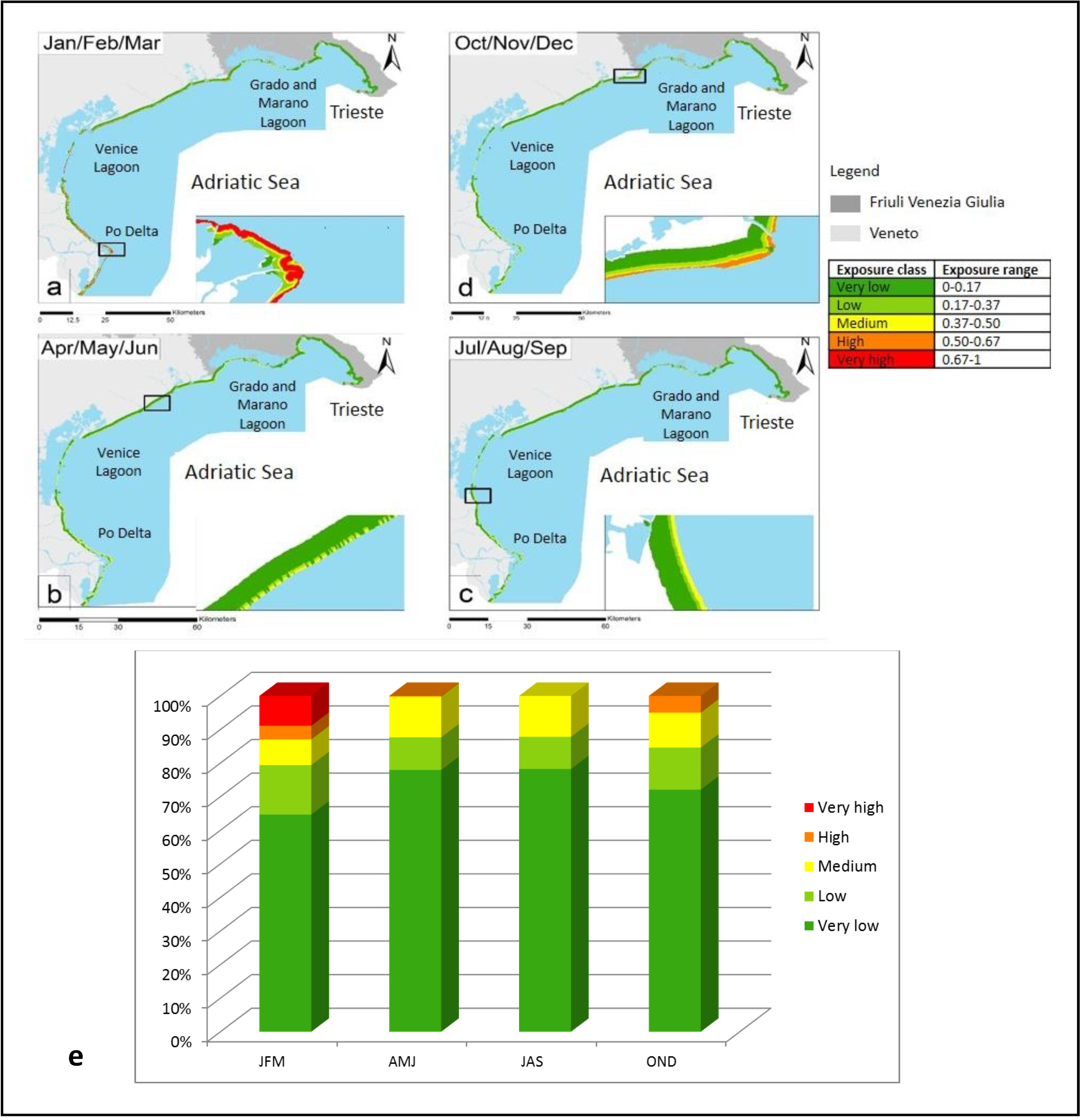
The exposure maps show how the exposure decreases moving inland from the shoreline, according to the increasing distance from the coast (Figure 2c). Moreover, the exposure is generally reduced where there is the presence of artificial protections (zoom of Figure 2b). Finally, it is possible to see that the exposure maps reproduce the main seasonal distribution of hazard metrics highlighted in the hazard scenarios (Figure S1). The seasons most affected by higher exposure classes are winter (January/February/March) and autumn (October/November/December). In winter the area more exposed to the hazard is the Po river delta (Figure 2a) where both the hazard metrics assumed the score 1. In autumn a higher exposure is observed near the Grado-Marano lagoon (Figure 2d). This situation is mainly due to the combined higher hazard scores gained by wave height and bottom stress in that area.
Figure 2e provides a comparison of the exposure classes within the RICE area in the 4 seasons: the territory potentially exposed to the very high and high classes is about 0.2% in spring, 5% in autumn and 12% in winter; the territory associated to the very low exposure classes is about 65–78% in all scenarios.

4.2. Susceptibility Maps

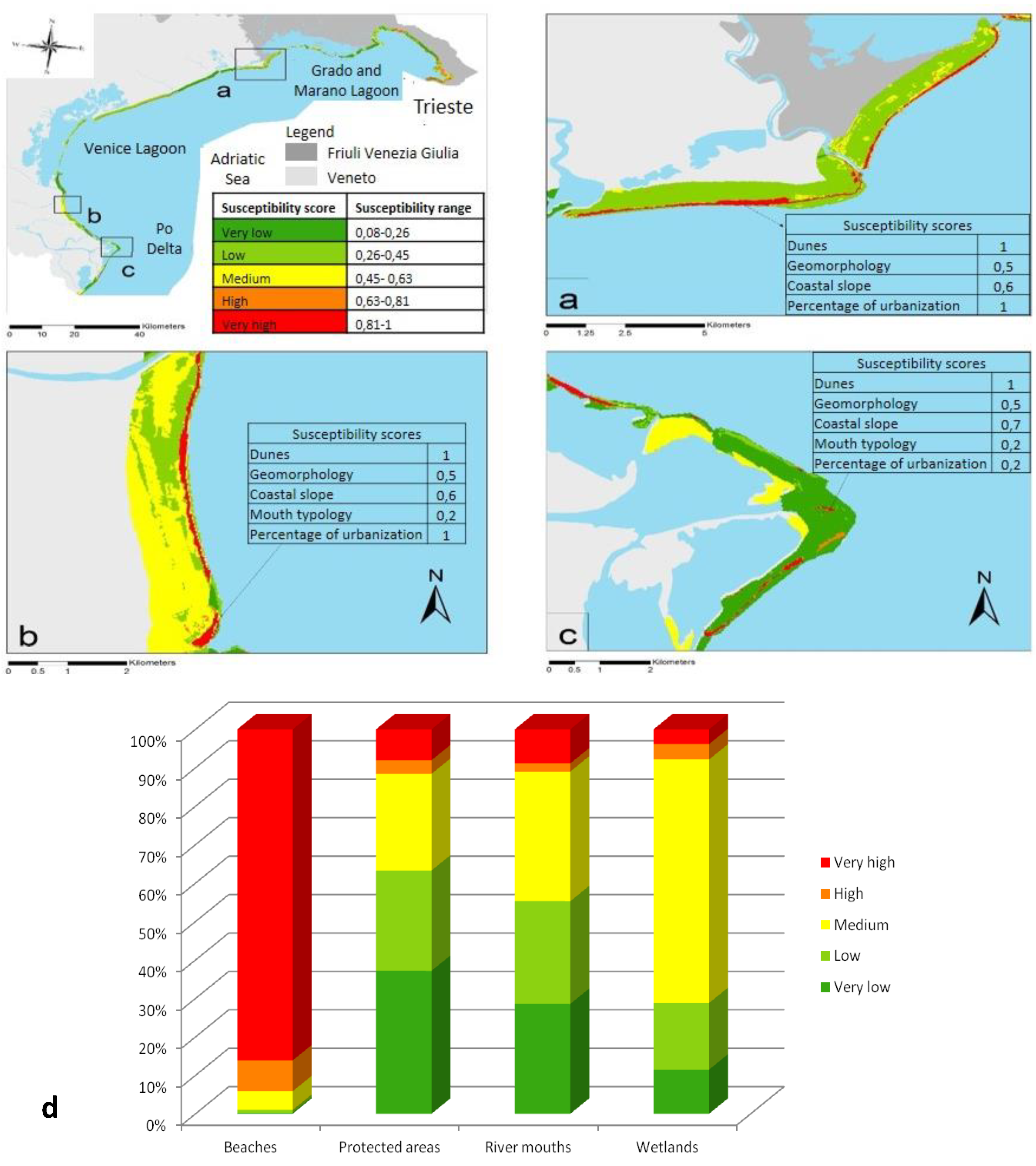
Figure 3 shows the distribution of susceptibility scores in the RICE area and the percentage of receptors within each susceptibility class. Areas with higher susceptibility scores are located in the southern part of the Venice Lagoon and near the Tagliamento river mouth due to the high percentage of urbanization and to the absence of dunes that makes the areas more prone to coastal erosion (Figure 3a,b).
Lower susceptibility areas in Figure 3a are flatlands that have a lower contribution to the susceptibility (score 0.2) and a high weight (0.8). In Figure 3b the territory is mainly in the medium susceptibility class due to the lower score (0.2) associated to coastal slope, mouth typology and wetland extension. Moreover, the area near the Po Delta (Figure 3c) shows higher susceptibility values due to high scores related to the absence of dunes (susceptibility score equal to 1 and weight 0.6) characterizing the littoral area of the NA region, and to the geomorphology that in this area is mainly represented by sandy areas (susceptibility score equal to 0.5 and weight 0.8). Lower susceptibility of the flatland delta area is due to the lower susceptibility (0.2) associated to slope and to the relatively low percentage of urbanization.
Figure 3d highlights that beach is the receptor more susceptible to coastal erosion (with about 94% of the territory in the very high and high susceptibility class), followed by protected areas and river mouths (with a value of about 11%), and finally by wetlands (8%).
Wetlands show more percentage of the territory in the medium susceptibility class (63%), while protected areas have higher surface percentage (63%) in the low and very low classes. In general, susceptibility factors contributing more to the final susceptibility score are geomorphology, coastal slope and shoreline variations, which gained higher weights in the assessment.

4.3. Risk Maps

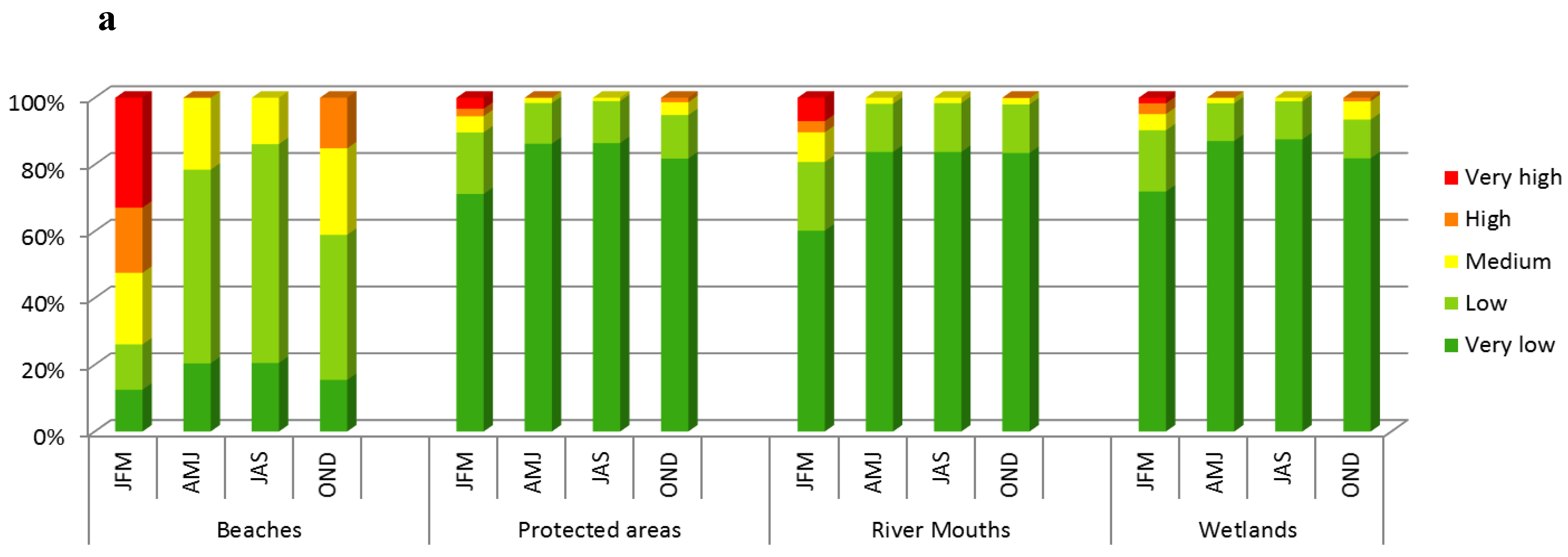
According to Figure 4a, the beaches show the higher percentage of surface in the higher risk classes (very high, high and medium), in all the analysed scenarios; this is basically due to their high susceptibility (Section 4.2). The winter trimester is the scenario in which the risk score is higher compared to the other seasons, this is due to the relatively higher values assumed by wave height and bottom stress in this scenario.
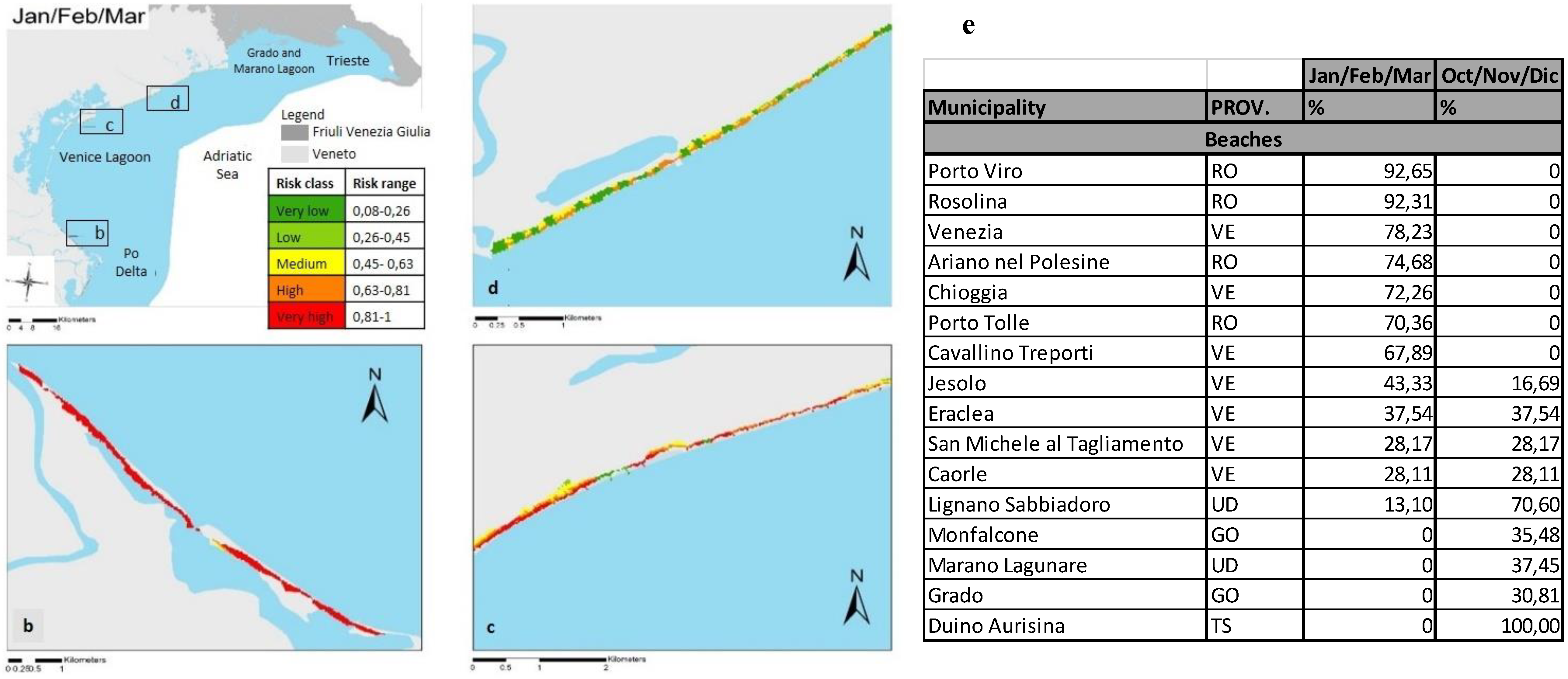
Figure 4 shows the future risk pattern in 2070–2100 for some selected areas (b, c and d) in the worst seasonal scenario (the winter trimester). The area along the Po River Delta (Figure 4b) includes beaches at very high risk. Some areas located along the Veneto coastline (Figure 4c,d) show the influence of artificial protections in decreasing the final risk scores.
In general agreement with these findings, Bonaldo et al. [66] applied the wave fields adopted in this study to a nearshore hydro-morphodynamic model (MIKE LITPACK) in the NA region. With reference to an intermediate emission scenario, they found an overall decrease of the wave energy impacting the coast, especially in the case of extreme storms. As a consequence, beach profiles are expected to undergo milder modifications in response to single events, but the predicted reduction of long-shore sediment drift (and a different modulation of its long-shore gradients) over a wide range of time scales may have significant implications in terms of coastline evolution. For this reason, a rigorous approach to coastal management should include the estimate, in a climate change scenario, of all the main forcing factors concurring to coastal landscape evolution, such as wave climate, riverine sediment supply and relative sea level rise as well.
Figure 4e shows the the percentage of beaches with very high/high risk scores in the coastal municipalities, for the winter and autumn trimesters. These are the municipalities where priority actions for adaptation should be developed (e.g., measures for the prevention of beach erosion or their preservation/restoration). In winter, Porto Viro and Rosolina show about 92% of beaches in the higher risk class, followed by Venice with about 78.23%. Also Ariano nel Polesine, Chioggia, Porto Tolle and Cavallino Treporti are characterized by relatively high percentages of beaches (from 68 to 75%) in the higher risk class. In autumn, the 100% of beaches in Duino Aurisina municipality would be at risk, followed by those located in Lignano Sabbiadoro (70.6%).
Risk statistics and maps can be used as a quick scan tool to rank areas and municipalities requiring higher attention for the implementation of coastal zone management and adaptation strategies (e.g., coastal sediment management plans, designation of strategic sediment reservoirs, restoring of the sediment balance). They can be used to set priorities for the allocation of further financial and technical support (e.g., for the definition of hot-spot areas requiring quantitative and site-specific risk analysis).

4.4. Damage Maps

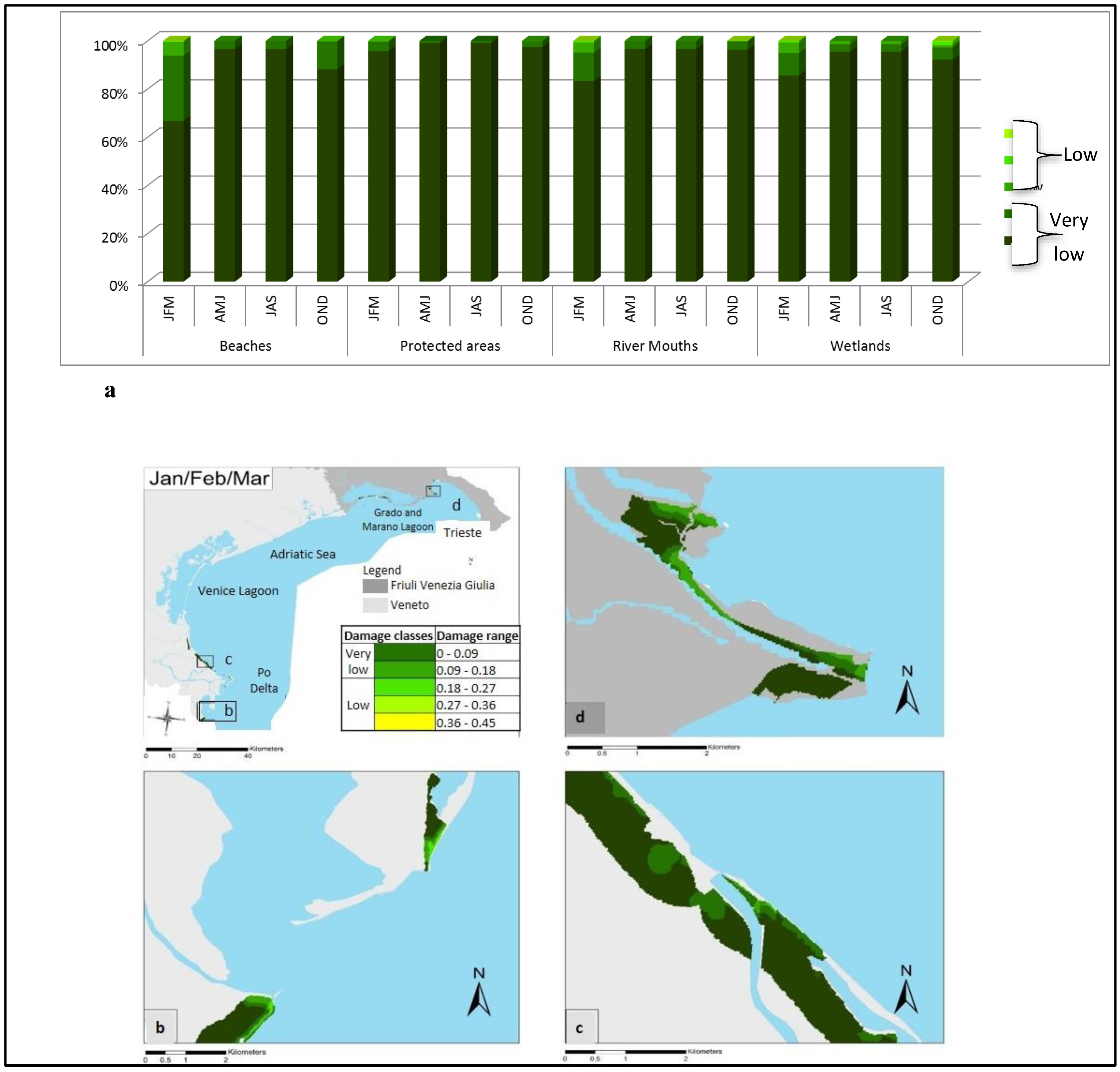
Figure 5 highlights the percentage of receptors’ surface in the damage classes, showing an example of map for the wetlands. For the majority of receptors, the territory in the lower damage class is the most relevant. The worst situation occurs in winter, due to the higher risk scores in this season. Overall, the damage maps have scores ranging from 0 to 0.45 (very low and low damage classes). A graduated shading of greens has been used for a better visualization of the pattern of classes in the territory. Despite relatively high risk scores, the damage classes are low in about 77% of the territory, due to the presence of value factors with relatively low scores (e.g., Nature 2000 areas, low population living in residential areas, Table S7 and Figure S2). Few areas with higher damage classes are located near protected areas (e.g., Isonzo mouth Park, Figure 5d). In these areas special attention should be paid to the potential loss of ecosystems (both in physical and ecological terms) and to the associated negative socio-economic consequences for the coastal community. Therefore, damage maps could support the NA municipalities in the planning of prevention measures aimed at avoiding future costs of inaction.

5. Conclusions

The strength of this relative risk assessment methodology is its applicability to different case studies as it can be tailored to different geographic and administrative contexts thanks to the transparency within each step of the assessment, and the flexibility to use different data for specific areas. Moreover, the assessment of climate change impact on coastal erosion was done using a bi-dimensional relative risk index, while similar assessments are usually applied to rank one-dimensional segments along the shoreline. The same methodological approach can also be easy adapted and replicated for the assessment of other climate-related impacts (e.g., pluvial floods) [27].
One of the limits of such approach is that potential processes leading to coastal erosion are analysed using proxies (e.g., wave height and bottom stress), neglecting some important factors (e.g., sediment supply from rivers, local effect of dikes). Therefore, the results do not allow an accurate estimation of future erosion rates along the shoreline for specific locations. However, the outcomes of this first work on the NA region indicate the feasibility of coupling an integrated numerical downscaling approach with regional risk assessment studies, in order to support the assessment and management of climate change impacts in coastal areas. In fact, regional-scale approximations combined with robust empirical risk and vulnerability modelling could provide support for risk assessors involved in decision-making processes over wide spatial extents [67].
Until now, coastal erosion was assessed by CVI or similar methods considering historical dataset of erosion processes. In this study, the use of future numerical model simulations allows to evalaute the impact of climate change on coastal systems in the longer term (2070–2100), supporting adaptation planning, as suggested by the IPCC [68].
Clearly, the issues of model validation are particularly relevant when dealing with long-term or multi-year simulations under climate change scenarios. For a critical discussion about limits of such approaches, including the potential dynamical downscaling strategies, the readers should refer to Torresan et al. [30].
The work presented in this paper should be considered as a testing of the RRA methodology, providing a first ranking of areas/targets where climate change could potentially affect coastal erosion drivers (and related risks) in the study area, and an overview of the functionalities that can be offered to local stakeholders for Integrated Coastal Zone Management (ICZM). The regional risk maps could be easily implemented in different coastal areas and case studies, and tailored to the objectives and policy needs of coastal authorities and decision-makers.

Supplementary Materials

The following are available online at https://www.mdpi.com/2073-4441/11/6/1300/s1, Figure S1: Hazard Maps representing the number of events exceeding the wave height threshold of 0.97 m (a–d); and the number of events exceeding the bottom stress threshold of 0.15 N/m2 (e–h) in the future scenario 2070–2100 in the four seasons (April/May/June, July/August/September, October/ November/December, January/February/March). Adapted from Torresan et al. [30], Figure S2: Value map for three selected protected areas (a–c) within the RICE area for the North Adriatic coast for the coastal erosion impact; and distribution of the territorial surface (km2) (d) and of the percentage of surface (e) that is associated with each value class for the receptors located in the North Adriatic coasts within the RICE area for the coastal erosion impact, Table S1: Exposure equations applied in the Exposure function, Table S2: Classes and scores associated with the hazard metrics identified in the hazard matrix for the coastal erosion impact in the North Adriatic coast. Each class represent a range of wave height and bottom stress events exceeding the thresholds identified in the reference period (i.e., 0.97 m and 0.15 N/m2 respectively), Table S3: Qualitative evaluations supporting the expert/decision maker in the assignation of relative scores to vulnerability and hazard classes (source: [67]), Table S4: Classes and scores associated with the susceptibility factors identified in the vulnerability matrix for the coastal erosion impact in the North Adriatic coast, Table S5: Weights associated with the susceptibility factors identified in the vulnerability matrix for the coastal erosion impact in the North Adriatic coast, Table S6: Classes and scores associated with the value factors identified in the vulnerability matrix for the coastal erosion impact, Table S7: Surface (km2) and percentage of Nature 2000 and Regional protection areas for the municipalities interested by damage in the North Adriatic coast within the RICE area for the coastal erosion impact (for the first semester of the thirty-year future scenario).

Author Contributions

Conceptualization, V.G., S.T., A.Z., L.P., A.M. and A.C.; Data curation, V.G., S.T., J.R. and S.C.; Formal analysis, V.G., S.T., J.R., S.C. and A.C.; Methodology, V.G., S.T., A.Z., J.R., L.P. and A.C.; Supervision, M.S., A.M. and A.C.; Writing—original draft, V.G., S.T., S.C. and A.C.; Writing—review & editing, V.G., S.T. and A.C.

Funding

The research leading to these results has received funding from the Italian Ministry of Education, University and Research and the Italian Ministry of Environment, Land, and Sea under GEMINA project.

Acknowledgments

The authors thank their colleagues Paolo Riccato and Elisa Furlan for the technical assistance with the GIS application.

Conflicts of Interest

The authors declare no conflict of interest.

References

  1. IPCC. Summary for policymakers. In Climate Change 2014: Impacts, Adaptation, and Vulnerability. Part A: Global and Sectoral Aspects. Contribution of Working Group II to the Fifth Assessment Report of the Intergovernmental Panel on Climate Change; Field, C.B., Barros, V.R., Dokken, D.J., Mach, K.J., Mastrandrea, M.D., Bilir, T.E., Chatterjee, M., Ebi, K.L., Estrada, Y.O., Genova, R.C., et al., Eds.; Cambridge University Press: Cambridge, UK; New York, NY, USA, 2014; pp. 1–32. [Google Scholar]
  2. EEA. Report No. 1/2017. Climate Change, Impacts and Vulnerability in Europe 2016. An Indicator-Based Report; EEA: Copenhagen, Denmark, 2017; ISSN 1977-8449. [Google Scholar]
  3. IPCC. Climate Change 2013: The Physical Science Basis. In Contribution of Working Group I to the Fifth Assessment Report of the Intergovernmental Panel on Climate Change; Stocker, T.F., Qin, D., Plattner, G.-K., Tignor, M., Allen, S.K., Boschung, J., Nauels, A., Xia, Y., Bex, V., Midgley, P.M., Eds.; Cambridge University Press: Cambridge, UK; New York, NY, USA, 2013; 1535p. [Google Scholar]
  4. Gualdi, S.; Somot, S.; Li, L.; Artale, V.; Adani, M. The CIRCE simulations: A new set of regional climate change projections performed with a realistic representation of the Mediterranean Sea. Bull. Am. Meteorol. Soc. 2013, 94, 65–81. [Google Scholar] [CrossRef]
  5. Lovato, T.; Vichi, M.; Oddo, P. High resolution simulations of Mediterranean Sea physical oceanography under current and scenario climate conditions: Model description, assessment and scenario analysis. CMCC Res. Pap. 2013, 1–26. [Google Scholar] [CrossRef]
  6. Colin, R.T.; Evans, E.P.; Penning-Rowsell, E.C. Future Flooding and Coastal Erosion Risks; Thomas Telford Publishing, Thomas Telford Ltd.: London, UK, 2007; p. 256. ISBN 978-0-7277-3449-5. [Google Scholar]
  7. IPCC. Summary for Policymakers. In Climate Change 2007: Impacts, Adaptation and Vulnerability. Contribution of Working Group II to the Fourth Assessment Report of the Intergovernmental Panel on Climate Change; IPCC: Geneva, Switzerland, 2007. [Google Scholar]
  8. Australian Government. Climate Change Risks to Australia’s Coast. A First Pass National Assessment; Australian Government: Canberra, Australia, 2009; ISBN 978-1-921298-71-4.
  9. EC. Living with Coastal Erosion in Europe: Sediment and Space for Sustainability; Part I—Major Findings and Policy Recommendations of the EUROSION Project; EUCC: Leiden, The Netherlands, 2004. [Google Scholar]
  10. Vafeidis, A.T.; Nicholls, R.J.; McFadden, L.; Tol, R.S.J.; Hinkel, J.; Spencer, T.; Grashoff, P.S.; Boot, G.; Klein, R.J.T. A New Global Coastal Database for Impact and Vulnerability Analysis to Sea-Level Rise. J. Coast. Res. 2008. [Google Scholar] [CrossRef]
  11. Bruun, P. Sea-level rise as a cause of shore erosion: Proceedings of the American Society of Civil Engineers. J. Waterw. Harb. Div. 1962, 88, 117–130. [Google Scholar]
  12. CEAC. Final Technical Report Development of Coastal Erosion Hazard Maps San Pedro, Belize; CEAC: Kingston, Jamaica, 2006.
  13. Harvey, N.; Woodroffe, C.D. Australian approaches to coastal vulnerability assessment. Sustain. Sci. 2008, 3, 67–87. [Google Scholar] [CrossRef]
  14. Sharples, C. Indicative Mapping of Tasmanian Coastal Vulnerability to Climate Change and Sealevel Rise: Explanatory Report, 2nd ed.; Department of Primary Industries, Water & Environment: Hobart, Australia, 2006; 112p.
  15. Abuodha, P.A.O.; Woodroffe, C.D. Assessing Vulnerability of Coast to Climate Change: A Review of Approaches and Their Application to the Australian Coast; University of Wollongong, Faculty of Science Papers: Wollongong, Australia, 2006. [Google Scholar]
  16. Gornitz, V.M.; Daniels, R.C.; White, T.W.; Birdwell, K.R. The Development of a Coastal Risk Assessment Database: Vulnerability to Sea-Level Rise in the U.S. Southeast; U.S. Government Report DE-AC05-84OR21400; Oak Ridge National Laboratory: Oak Ridge, TN, USA, 1993.
  17. Ramieri, E.; Hartley, A.; Barbanti, A.; Duarte Santos, F.; Gomes, A.; Hilden, M.; Laihonen, P.; Marinova, N.; Santini, M. Methods for Assessing Coastal Vulnerability to Climate Change; European Topic Centre on Climate Change Impacts, Vulnerability and Adaptation (ETC CCA) Technical Paper; European Environment Agency: Bologna, Italy, 2011; p. 93. [Google Scholar]
  18. Torresan, S.; Critto, A.; Dalla Valle, M.; Harvey, N.; Marcomini, A. Assessing coastal vulnerability to climate change: Comparing segmentation at global and regional scales. Sustain. Sci. 2008, 3, 45–65. [Google Scholar] [CrossRef]
  19. Idier, D.; Castelle, B.; Poumadere, M.; Balouin, Y.; Bertoldo, R.B.; Bouchette, F.; Boulahya, F.; Brivois, O.; Calvete, D.; Capo, S.; et al. Vulnerability of sandy coasts to climate variability. Clim. Res. 2013, 57, 19–44. [Google Scholar] [CrossRef] [Green Version]
  20. Di Paola, G.; Aucelli, P.P.; Benassai, G.; Rodríguez, G. Coastal vulnerability to wave storms of Sele littoral plain (southern Italy). Nat. Hazards 2014, 71, 1795–1819. [Google Scholar] [CrossRef]
  21. Hereher, M.E. Coastal vulnerability assessment for Egypt’s Mediterranean coast. Geomat. Nat. Hazards Risk 2015, 6, 342–355. [Google Scholar] [CrossRef]
  22. Satta, A.; Snoussi, M.; Puddu, M.; Flayou, L.; Hout, R. An index-based method to assess risks of climate-related hazards in coastal zones: The case of Tetouan. Estuar. Coast. Shelf Sci. 2016. [Google Scholar] [CrossRef]
  23. Pantusa, D.; D’Alessandro, F.; Riefolo, L.; Principato, F.; Tomasicchio, G.R. Application of a coastal vulnerability index. A case study along the Apulian Coastline, Italy. Water 2018, 10, 1218. [Google Scholar] [CrossRef]
  24. Landis, W.G. Regional Scale Ecological Risk Assessment. Using the Relative Risk Model; Landis, W.G., Ed.; CRC Press: Boca Raton, FL, USA, 2005. [Google Scholar]
  25. Zanuttigh, B.; Simcic, D.; Bagli, S.; Bozzeda, F.; Pietrantoni, L.; Zagonari, F.; Hoggart, S.; Nicholls, R.J. THESEUS decision support system for coastal risk management. Coast. Eng. 2014, 87, 218–239. [Google Scholar] [CrossRef]
  26. Hagenlocher, M.; Renaud, F.G.; Haas, S.; Sebesvari, Z. Vulnerability and risk of deltaic social-ecological systems exposed to multiple hazards. Sci. Total Environ. 2018, 631–632, 71–80. [Google Scholar] [CrossRef] [PubMed]
  27. Sperotto, A.; Torresan, S.; Gallina, V.; Coppola, E.; Critto, A.; Marcomini, A. A multi-disciplinary approach to evaluate pluvial floods risk under changing climate: The case study of the municipality of Venice (Italy). Sci. Total Environ. 2016, 562, 1031–1043. [Google Scholar] [CrossRef]
  28. Ronco, P.; Zennaro, F.; Torresan, S.; Critto, A.; Santini, M.; Trabucco, A.; Zollo, A.L.; Galluccio, G.; Marcomini, A. A risk assessment framework for irrigated agriculture under climate change. Adv. Water Resour. 2017, 110, 562–578. [Google Scholar] [CrossRef]
  29. Sanuy, M.; Duo, E.; Jäger, W.S.; Ciavola, P.; Jiménez, J.A. Linking source with consequences of coastal storm impacts for climate change and risk reduction scenarios for Mediterranean sandy beaches. Nat. Hazards Earth Syst. Sci. 2018. [Google Scholar] [CrossRef]
  30. Torresan, S.; Gallina, V.; Gualdi, S.; Bellafiore, D.; Umgiesser, G.; Carniel, S.; Sclavo, M.; Benetazzo, A.; Giubilato, E.; Critto, A. Assessment of climate change impacts in the North Adriatic coastal area. Part I: A multi-model chain for the definition of climate change hazard scenarios. Water 2019, 11, 1157. [Google Scholar] [CrossRef]
  31. Torresan, S.; Critto, A.; Rizzi, J.; Zabeo, A.; Furlan, E.; Marcomini, A. DESYCO: A decision support system for the regional risk assessment of climate change impacts in coastal zones. Ocean Coast. Manag. 2016, 120, 49–63. [Google Scholar] [CrossRef]
  32. Antonioli, F.; Anzidei, M.; Amorosi, A.; Lo Presti, V.; Mastronuzzi, G.; Deiana, G.; De Falco, G.; Fontana, A.; Fontolan, G.; Lisco, S.; et al. Sea-level rise and potential drowning of the Italian coastal plains: Flooding risk scenarios for 2100. Quat. Sci. Rev. 2017. [Google Scholar] [CrossRef]
  33. Marsico, A.; Lisco, S.; Lo Presti, V.; Antonioli, F.; Amorosi, A.; Anzidei, M.; Deiana, G.; De Falco, G.; Fontana, A.; Fontolan, G.; et al. Flooding scenario for four italian coastal plains using three relative sea level rise models. J. Maps 2017. [Google Scholar] [CrossRef]
  34. Carbognin, L.; Teatini, P.; Tomasin, A.; Tosi, L. Global change and relative sea level rise at Venice: What impact in term of flooding. Clim. Dyn. 2009, 35, 1039–1047. [Google Scholar] [CrossRef]
  35. Tomasin, A.; Pirazzoli, P.A. Extreme Sea Levels on the Adriatic Coasts: A Comparison of Estimation Methods; Atti dell’Istituto Veneto di Scienze, Lettere ed Arti Tomo CLXVII (2008–2009); Istituto Veneto di Scienze, Lettere ed Arti: Venice, Italy, 2008; pp. 53–82. [Google Scholar]
  36. Umgiesser, G.; Anderson, J.B.; Artale, V.; Breil, M.; Gualdi, S.; Lionello, P.; Marinova, N.; Orlić, M.; Pirazzoli, P.; Rahmstorf, S.; et al. From Global to regional: Local Sea Level Rise Scenarios. Focus on the Mediterranean Sea and the Adriatic Sea; Workshop Report n.1; United Nations Educational Scientific and Cultural Organization (UNESCO): Paris, France, 2011; p. 25. [Google Scholar]
  37. Rizzi, J.; Torresan, S.; Zabeo, A.; Critto, A.; Tosoni, A.; Tomasin, A.; Marcomini, A. Assessing storm surge risk under future sea-level rise scenarios: A case study in the North Adriatic coast. J. Coast. Conserv. 2016. [Google Scholar] [CrossRef]
  38. Ferretti, O.; Delbono, I.; Furia, S.; Barsanti, M. Elementi di Gestione Costiera Parte Prima Tipi Morfo-Sedimentologici dei Litorali Italiani; RT/2003/42/CLIM; ENEA: Rome, Italy, 2003; ISSN 0393-3016. [Google Scholar]
  39. Cecconi, G. The VeniceLagoon mobile barriers. Sea level rise and impact of barrier closures. In Proceedings of the Italian Days of Coastal Engineering, International Debate-PIC 97, Venice, Italy, 16 May 1997. [Google Scholar]
  40. Cecconi, G.; Ardone, V. La protezione dei litorali con ripascimento delle spiagge. L’esperienza dei litorali di Cavallino e Pellestrina. In Proceedings of the La progettazione ambientale nei sistemi costieri, a cura di M. Pietrobelli, Atti del X Seminario, Roma, Italy, 10 July 1998; International Association for Environmental Design (IAED, Quaderno 12); pp. 11–31. [Google Scholar]
  41. CVN. La fonte di Approvvigionamento della Sabbia nel Ripascimento dei Litorali Veneti; Cecconi, G., Ardone, V., Eds.; Consorzio Venezia Nuova: Venezia, Italy, 2000. [Google Scholar]
  42. Cecconi, G.; Ardone, V. La fonte di Approvvigionamento della Sabbia nel Ripascimento dei Litorali Veneti, Intervento alla Presentazione della Costa Ligure; Regione Liguria: Genova, Italy, 2–4 February 2000. [Google Scholar]
  43. Visintini Romanin, M.; Rismondo, A.; Scarton, F.; Leita, L. Interventi per il recupero morfologico della laguna di Venezia. La barena Fossei Est in laguna Sud. Quad. Trimest. 2000, 3–4, 3–35. [Google Scholar]
  44. Regione, F.V.G. Piano di gestione del SIC IT3320037 Laguna di Grado e Marano. Carta delle aree di Tutela e di Intervento scala 1:50,000; Agriconsulting: Friuli Venezia Giulia Region, Italy, 2008. [Google Scholar]
  45. Fagherazzi, S.; Wiberg, P.L. Importance of wind conditions, fetch, and water levels on wave-generated shear stresses in shallow intertidal basins. J. Geophys. Res. 2009, 114, F03022. [Google Scholar] [CrossRef]
  46. Özyurt, G. Vulnerability of Coastal Areas to Sea Level Rise: Case Study on Goksu Delta. Master’s Thesis, Middle East Technical University, Ankara, Turkey, 2007. [Google Scholar]
  47. Carniel, S.; Sclavo, M.; Archetti, R. Towards validating a last generation, integrated wave-current-sediment numerical model in coastal regions using video measurements. Oceanol. Hydrobiol. Stud. 2011, 40, 11–20. [Google Scholar] [CrossRef]
  48. Benetazzo, A.; Carniel, S.; Sclavo, M.; Bucchignani, E.; Ricchi, A. Wave climate of the Adriatic Sea: A future scenario simulation. Nat. Hazards Earth Syst. Sci. 2012, 12, 2065–2076. [Google Scholar] [CrossRef]
  49. Torresan, S.; Critto, A.; Rizzi, J.; Marcomini, A. Assessment of coastal vulnerability to climate change hazards at the regional scale: The case study of the North Adriatic Sea. Nat. Hazards Earth Syst. Sci. 2012, 12, 2347–2368. [Google Scholar] [CrossRef]
  50. VE Region. Map of National and Regional Established Parks, Environmental Planning and Parks Unit. 2006. Available online: http://idt.regione.veneto.it/app/metacatalog/ (accessed on 16 June 2019). (In Italian).
  51. FVG Region. Digital Elevation Model (DEM) for the Friuli Venezia Giulia Region, Geographic Information System and Cartography Unit. 2006. Available online: http://irdat.regione.fvg.it/consultatore-dati-ambientali-territoriali/ (accessed on 16 June 2019). (In Italian).
  52. FVG Region. Monitoring Land Use/Cover Dynamics (MOLAND) Map for the Friuli Venezia Giulia Region, Geographic Information System and Cartography Unit. 2000. Available online: http://irdat.regione.fvg.it/consultatore-dati-ambientali-territoriali/ (accessed on 16 June 2019). (In Italian).
  53. VE Region. Regional Land cover Map based on Corine Land Cover legend, Geographic Information System and Cartography Unit. 2009. Available online: http://idt.regione.veneto.it/app/metacatalog/ (accessed on 16 June 2019). (In Italian).
  54. Nakićenovićet, N.; Alcamo, J.; Davis, G.; de Vries, H.J.M.; Fenhann, J.; Gaffin, S.; Gregory, K.; Grubler, A.; Jung, T.Y.; Kram, T.; et al. Special Report on Emissions Scenarios. Intergovernmental Panel on Climate Change; Cambridge University Press: Cambridge, UK, 2000. [Google Scholar]
  55. Booij, N.; Ris, R.C.; Holthuijsen, L.H. A third-generation wave model for coastal regions Part I Model description and validation. J. Geoph. Res. 1999, 104, 7649–7666. [Google Scholar] [CrossRef]
  56. Bergamasco, A.; Carniel, S.; Pastres, R.; Pecenik, G. A unified approach to the modelling of the Venice Lagoon–Adriatic Sea ecosystem. Estuar. Coast. Shelf Sci. 1998, 46, 483–492. [Google Scholar] [CrossRef]
  57. McLaughlin, S.; Cooper, J.A.G. A multi-scale coastal vulnerability index: A tool for coastal managers? Environ. Hazards 2010, 9, 233–248. [Google Scholar] [CrossRef]
  58. Zald, A.E.; Shelly, S.; Wade, T. A to Z GIS: An Illustrated Dictionary of Geographic Information Systems; ESRI Press: Beijing, China, 2006. [Google Scholar]
  59. Crozier, M.; Glade, T. Landslide hazard and risk: Issues, concepts and approach. In Landslide Hazard and Risk; Glade, T., Anderson, M., Crozier, M., Eds.; John Wiley & Sons, Ltd.: Chichester, UK, 2005; pp. 1–40. [Google Scholar]
  60. Kalbfleisch, J.G. Probability and Statistical Inference: Volume 1: Probability; Springer Science & Business Media: Berlin, Germany, 1985. [Google Scholar]
  61. Preston, B.L.; Smith, T.F.; Brooke, C.; Gorddard, R.; Measham, T.G.; Withycombe, G.; Mcinnes, K.; Abbs, D.; Beveridge, B.; Morrison, C. Mapping Climate Change Vulnerability in the Sydney Coastal Councils Group; Sydney Coastal Councils Group: Manly, Australia, 2008. [Google Scholar]
  62. ARC. Coastal Erosion Management Manual Technical Publication No. 130; ARC: Canberra, Australia, 2000. [Google Scholar]
  63. Eurosion. Living with Coastal Erosion in Europe: Sediment and Space for Sustainability. PART III—Methodology for Assessing Regional Indicators. 20 May 2004. Available online: http://www.eurosion.org/reportsonline/part3.pdf (accessed on 19 June 2015).
  64. Greiving, S.; Fleischhauer, M.; Lückenkötter, M. A Methodology for an Integrated Risk Assessment of Spatially Relevant Hazards. J. Environ. Plan. Manag. 2006, 49, 1–19. [Google Scholar] [CrossRef]
  65. EC. ARMONIA Project. Applied Multi-Risk Mapping of Natural Hazards for Impact Assessment; Deliverable 4.1.2. Report: Technical Glossary of a Multi Hazard Related Vulnerability and Risk Assessment Language—Final Version; EC: Brussels, Belgium, 2007. [Google Scholar]
  66. Bonaldo, D.; Benetazzo, A.; Sclavo, M.; Carniel, S. Modelling wave-driven sediment transport in a changing climate: A case study for northern Adriatic Sea (Italy). Reg. Environ. Chang. 2014. [Google Scholar] [CrossRef]
  67. Bosco, C.; de Rigo, D.; Dewitte, O.; Poesen, J.; Panagos, P. Modelling soil erosion at European scale: Towards harmonization and reproducibility. Nat. Hazards Earth Syst. Sci. 2015, 15, 225–245. [Google Scholar] [CrossRef]
  68. Klein, R.J.T.; Midgley, G.F.; Preston, B.L.; Alam, M.; Berkhout, F.G.; Dow, K.; Li, Y.E.; Mateescu, E.; Shaw, M.R.; Botzen, W.; et al. Adaptation opportunities, constraints, and limits. In Climate Change 2014: Impacts, Adaptation, and Vulnerability. Part A: Global and Sectoral Aspects. Contribution of Working Group II to the Fifth Assessment Report of the Intergovernmental Panel on Climate Change; Field, C.B., Barros, V.R., Dokken, D.J., Mach, K.J., Mastrandrea, M.D., Bilir, T.E., Chatterjee, M., Ebi, K.L., Estrada, Y.O., Genova, R.C., et al., Eds.; Cambridge University Press: Cambridge, MA, USA; New York, NY, USA, 2014; pp. 899–943. [Google Scholar]
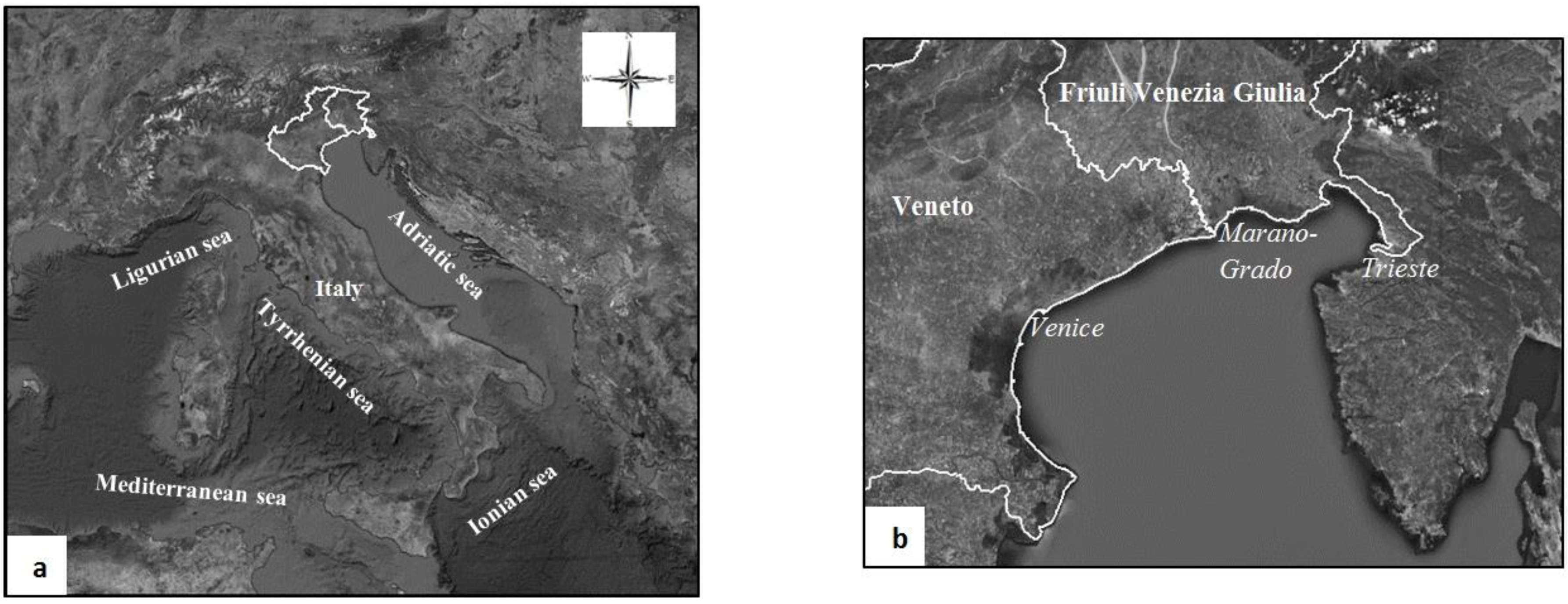
Figure 1. (a) Location of the study area in the North Eastern Italy; (b) the coast of Veneto and Friuli Venezia Giulia regions in the Northern Adriatic Sea (adapted from Google Maps: maps.google.it).
Water 11 01300 g001
Figure 2. Exposure map (ad); and distribution of the percentage of surface (e) associated with each exposure class for the North Adriatic coasts within the RICE area for the four seasons of the future scenario 2070–2100: January-February-March (JFM); April-May-June (AMJ); July-August-September (JAS); October-November-December (OND).
Water 11 01300 g002
Figure 3. Susceptibility maps relative to three selected regions (ac). The tables in the zooms sumarise the susceptibility factors responsible for the higher susceptibility score in the analyzed area; and distribution of the percentage of surface (d) associated with each susceptibility class for the each receptor located in the RICE area.
Water 11 01300 g003
Figure 4. Percentage of receptors’ surface in each risk class for the 4 seasons (January-February-March JFM; April-May-June AMJ; July-August-September JAS; October-November-December OND) of the future scenario 2070–2100 (a); example of risk map for beaches in the trimester Jan/Feb/Mar (bd); percentage of beach surface in the higher risk classes for the coastal municipalities in the NA study area (e).
Water 11 01300 g004aWater 11 01300 g004b
Figure 5. Percentage of receptors’ surface in each damage class for the 4 seasons (January-February-March JFM; April-May-June AMJ; July-August-September JAS; October-November-December OND) of the future scenario 2070–2100 (a); example of damage map for wetlands in the trimester Jan/Feb/Mar (bd).
Water 11 01300 g005
Table 1. Hazard matrix representing coastal erosion stressors and hazard metrics (light cells).
Hazard Matrix
StressorsClimate change impact
Bottom stresswave
Bottom stressHeightCoastal erosion
Table 2. Vulnerability matrix showing coastal receptors and vulnerability factors applied for the Regional Risk Assessment of coastal erosion in the North Adriatic coast.
ReceptorsBeachesRiver MouthsWetlands Protected Areas
Impact
Coastal erosion - Distance from coastline- Distance from coastline- Distance from coastline- Distance from coastline
- Artificial protections- Artificial protections- Artificial protections- Artificial protections
- Vegetation cover- Vegetation cover- Vegetation cover- Vegetation cover
- Coastal slope- Geomorphology- Geomorphology- Geomorphology
- Geomorphology- Sediment budget- Sediment budget- Sediment budget
- Sediment budget- Mouth typology- Wetland extension- % of urbanization
- Dunes- Protection level- % of urbanization- Protection level
- % of urbanization- Population density- Protection level- Population density
- Protection level- Urban typology- Population density- Urban typology
- Population density- Agricultural typology- Wetland extension- Agricultural typology
Legend
Vulnerability FactorsDefinition
Pathway factors (pf)Physical characteristics of the receptors (i.e., distance from coastline) which determine the possibility that coastal erosion reach receptors.
Attenuation factors (af)Elements that could attenuate the intensity of the coastal erosion (i.e., artificial protections).
Susceptibility factors (sf)Geo-physical or ecological factors used to determine the susceptibility of a receptor to coastal erosion (e.g., vegetation cover, coastal slope, geomorphology, dunes, sediment budget).
Value factors (vf)Relevant environmental and socio-economic values of the receptors that need to be preserved for the interest of the community (e.g., protection level, population density).
Table 3. Dataset used for the implementation of the regional risk assessment methodology in the NA study area. The acronym FVG means Friuli Venezia Giulia, ISPRA means High Institute for Environmental Protection and Research. Adapted from [49].
Vulnerability FactorDefinitionDataset (Source)
Pathway factor
Distance from coastline The distance of a location (e.g., a pixel of the map) from the coastline (km).25 m Digital Elevation Model (DEM) [50,51]
Attenuation factor
Artificial protectionArtificial protections (e.g., dikes) for the defence of the coastline from storm surge and coastal erosion impacts.Corine Land Cover, 1:100,000 [52,53]
Susceptibility factors
Vegetation coverThe typology of vegetation that cover an area (i.e., natural grassland and meadow, shrub, forest).Corine Land Cover, 1:100,000, Land use, 1:25,000 [52,53]
Coastal slope Average topographic slope (in degrees) along the coastline.25 m Digital Elevation Model (DEM) [50,51]
GeomorphologyGeomorphologic structure of the coastal zone. It refers to muddy (non consolidated), sandy or rocky coast typology.Geologic and Geomorphological Map of the Po river delta, 1:50,000 (Veneto Po Delta Regional Park Authority, https://www.parcodeltapo.org/index.php/it/)
DunesIt refers to the presence or absence of natural dunes.Corine Land Cover, 1:100,000 [52,53]
Sediment budgetIt refers to the morphological variations of coastlines (i.e., eroding advancing or stable shores).Geographic Coastal Information System (SIGC) (ISPRA, www.mais.sinanet.apat.it/cartanetms/coste/)
Mouth typologyIt refers to the type of river mouths (i.e., estuary, delta).Hydrologic basins: rivers and channels 1:25,000. [52]
(ISPRA, www.mais.sinanet.apat.it/cartanetms/)
Wetland extensionThe extent of wetlands in square kilometres (km2).Corine Land Cover, 1:100,000 [52,53]
% of urbanizationThe percentage of urbanized areas within each municipality.Corine Land Cover, 1:100,000, Land use, 1:25,000 [52,53]
Value factors
Protection levelIt refers to the type of protected areas within the considered receptor (i.e., national area, regional area, nature 2000 area).Protected Areas and ARIA zones, 1:150,000 [52]
Population density (inhabitants/km2)The average number of people who live on each square kilometre of land for each municipality.Census data [52,53]
Urban typologyThe typology of buildings (e.g., residential, commercial, infrastructures).Corine Land Cover, 1:100,000, Land use, 1:25,000 [52,53]
Agricultural typologyThe typology of farming in an area (e.g., permanent culture, stable meadow, arable).Corine Land Cover, 1:100,000, Land use, 1:25,000 [52,53]
Table 4. Equations applied for the assessment of climate change impact on coastal erosion risk in the NA coast.
EquationDescription
E c e , s = { 0                i f   p f 1 s 1 ( i = 1 n [ h c e , i , s ] ) ( 1 A t c e ) × d 1    o t h e r w i s e   (1)Exposure function is aimed at the relative ranking of areas potentially exposed to changes in coastal erosion stressors. It integrates information about the hazard metrics influenced by climate change (i.e., wave height and bottom stress, Paragraph 3.2), the presence of artificial protections and the distance from the sea.
where:
Ece,s = exposure score related to coastal erosion (ce) scenario s;
pf1 = pathway factor represented by the distance of the center of the cell from the sea (always ≥ 1 m);
s1 = threshold given by decision maker representing the distance of the coastline from the sea beyond which the erosion has no influence (m);
⊗ = “probabilistic or” function [60] (see Table S2);
hce,1,…,n,s = hazard metrics from 1 to n related to the coastal erosion impact classified and weighted in (0,1) through h′k,s = si,kwi,k where h′k,s = weighted hazard metric; si,k = score of the i-th hazard metric for the impact k; wi,k = weight of the i-th hazard metric for the impact k.
Atce = attenuation related to the presence of artificial protections (see Table S2);
d1 = distance from the shoreline calculated through a hyperbolic function (see Table S2).
S c e =   i n [ s f i , c e ]   (2)Susceptibility function is aimed at the aggregation of the major physical and environmental factors that may influence the response of the receptors to the hazard scenarios.
where:
Sce = susceptibility score of the cell to the coastal erosion ce;
⊗ = “probabilistic or” function (see Table S2);
sf’i,ce = ith susceptibility factor score related to the coastal erosion ce; and sf’i,ce = si,ce wi,ce, where sf’i,e = weighted susceptibility factor score; si,ce = score of the i-th susceptibility factor for the coastal erosion ce; wi,ce = weigh of the i-th susceptibility factor for the coastal erosion ce.
R c e , s = E c e , s × S c e   (3)Risk function is aimed at the integration of exposure and susceptibility information.
where:
Rce,s = risk score related to coastal erosion ce and scenario s; Ece,s = exposure score related with the coastal erosion ce in scenario s, according to Equation (1);
Sce= susceptibility score to the impact ce, according to Equation (2).
V j = i = 1 n [ v i , j ] n   (4)Value function is aimed at the identification and ranking of receptors with relevant environmental and socio-economic values that need to be preserved for the interest of the community (e.g., land use, agricultural areas).
where:
Vj = value score of the receptor j; vf’i,j = i-th value factor score related to the receptor j; and vf’ = si,j wi,j, where vf’ = weighted value factor score; si,j = score of the i-th factor for the receptor j; wi,j = weigh of the i-th factor for the receptor j; n = number of value factors.
D j , c e , s = R c e , s × V j   (5)Damage function is aimed at the integration of risk and value information.
where:
Dj,ce,s = damage score related to coastal erosion ce and a receptor j in the scenario s;
Rce,s = risk score related to coastal erosion ce in scenario s, according to Equation (3);
Vj = value score of receptor j, according to Equation (4).