Impact Analysis of Slope on the Head Loss of Gas-Liquid Two-Phase Flow in Siphon Pipe

Abstract

Through an analysis of the head loss of the gas–liquid two-phase flow in a siphon pipe, this paper measures the bubble velocity, pressure drop, and gas fraction under various conditions. The influence of varied head, gradient, and installation heights of the pipe on the air mass movement, head loss, and resistance coefficient of the gas–liquid two-phrase flow is analyzed on the basis of the test results. The results show that the bubble velocity reaches its minimum on the flat slope, and the velocity on the positive slope is higher than that on the reverse slope. The head loss of pipelines in both the positive slope and reverse slope increases as the gradient increases, while the head loss on the reverse slope is larger than that on the positive slope under the same gradient. When the gas fraction α is between 8% and 30%, the resistance coefficient λ_m is related to the gradient, gas fraction, and the Reynolds number Re. Furthermore, λ_m is proportionate to α and inversely proportionate to i of the bottom slope and the Re number. The calculation formula of the resistance coefficient λ_m under various gradients within the scope of the above gas fraction is derived on the basis of the test data, while the relative error is controlled within the allowable range.

1. Introduction

The construction of a long-distance water transfer project is one of the main measures used to alleviate the stress of water shortage [1,2,3]. Because it can be used in unconditional arrangements, the siphon has become the preferred choice for many projects. Domestic and foreign scholars have studied the mechanisms of siphon processes. For example, Petaccia et al. used pressure sensors and ultrasonic flowmeters to determine the hydraulic characteristics of siphons [4]. Naoki Tajima et al. described the phenomenon of particle movement in a siphon with the movement of water in a pipeline, and obtained the characteristics of the siphon [5,6]. Seo and Kang verified the design of a siphon breaker by experiment and numerical simulation. According to the size of the siphon break line, the undershooting height was measured and the pressure and surface velocity of the main pipe were analyzed according to the water level of the pool. Results showed good agreement with experimental results with a reasonable uncertainty range [7,8,9,10]. Through a sensitivity analysis, Jin proposed a mathematical model of flood risk across an inverted siphon in a long-distance water transfer project [11]. Diogo proposed a method for calculating two-phase flow in an inverted siphon pipe for sewage discharge and treatment, tested the method, and compared it with the data obtained in the siphon device experiment [12].

The calculation of resistance is one of the important topics in gas–liquid two-phase flow research, with the focus being on the study of pressure drop characteristics of two-phase flow and multi-phase flow in pressurized pipelines in recent years. Revellin et al. carried out a numerical simulation of gas–liquid two-phase flow in a horizontal circular pipe, spiral pipe, and t-shaped micro channel, and proposed the numerical solution under the gas–liquid two-phase uniform flow model [13,14]. Aliyu Musa et al. accurately established a model of the pressure drop and heat transfer coefficient in a gas–liquid two-phase flow pipe system and deduced the friction coefficient formula of the cross-section by studying the interface friction between gas and liquid in pipes [15,16]. Schmidt et al. proposed a method for measuring gas and liquid flow by observing a variety of gas–liquid two-phase flow patterns in v-shaped taper pipes [17,18]. Pietrzak et al. measured the pressure drop of gas–liquid three-phase flow in pipes, and proposed a new model to predict the pressure drop of three-phase flow [19,20,21]. Barnea et al. studied gas–liquid two-phase flow pattern transitions and drew a flow pattern map in horizontal and inclined pipes [22,23,24,25]. Pansunee et al. carried out experimental research on gas–liquid two-phase flow and pressure drop in micro channels, and proposed that the pressure drop was closely related to the flow pattern in pipes [26,27,28]. Gas–liquid two-phase flow could improve the heat transfer efficiency. The flow pressure drops increase with the increase of superficial velocity. Bhagwat studied the pressure drop of the gas–liquid two-phase flow in inclined pipes, and proposed that under the low flow velocity of the gas and liquid, the pipe obliquity has a great influence on the two-phase flow while the slip velocity of the gas–liquid interface greatly affects the friction pressure drop in pipes [29].

All the above studies were based on positive pressure pipelines, while there are few studies on two-phase and multi-phase flows under vacuum conditions. For multi-phase flow under negative pressure, this field is the most extensively researched in vacuum sewer systems [30,31]. Vacuum sewers involve complex movements of water, gas, and solid media, which is much more complicated than single-phase fluid flow [32,33]. Donald et al. simplified the multi-phase flow in vacuum sewers to Newtonian liquid single-phase flow, and the friction resistance of the pipeline was mainly calculated by the modified Hazen–Williams formula [34,35]. Duan et al. studied the two-phase flow friction pressure loss of gas–water mixed fluid in sewers, and obtained the affected factors to predict the friction pressure loss of multi-phase flow in sewage pipelines [36]. Siphon pipes operate under negative pressure conditions, and a few gas nuclei existing in raw water—which are invisible to the naked eye and insoluble in water—expand and separate out, leading to a greater internal pressure than external pressure. Therefore, the gas–liquid two-phase flow appears in siphon pipes when the influence of gas on pipeline pressure is different from that of the positive pressure pipes. This paper studies the pressure drop characteristics of the middle part of horizontal and inclined siphon pipes and determines the influence of the slope change on the air mass movement through tests. The dimensionless relation of pressure drop under air mass movement is obtained herein by means of dimensional analysis. Then, the paper reveals the influence mechanism of air mass movement characteristics on the head loss of gas–liquid two-phase flow in siphon pipes. The results lay a foundation for the computation theory of resistance and head loss of gas–liquid two-phase flow in siphon pipes.

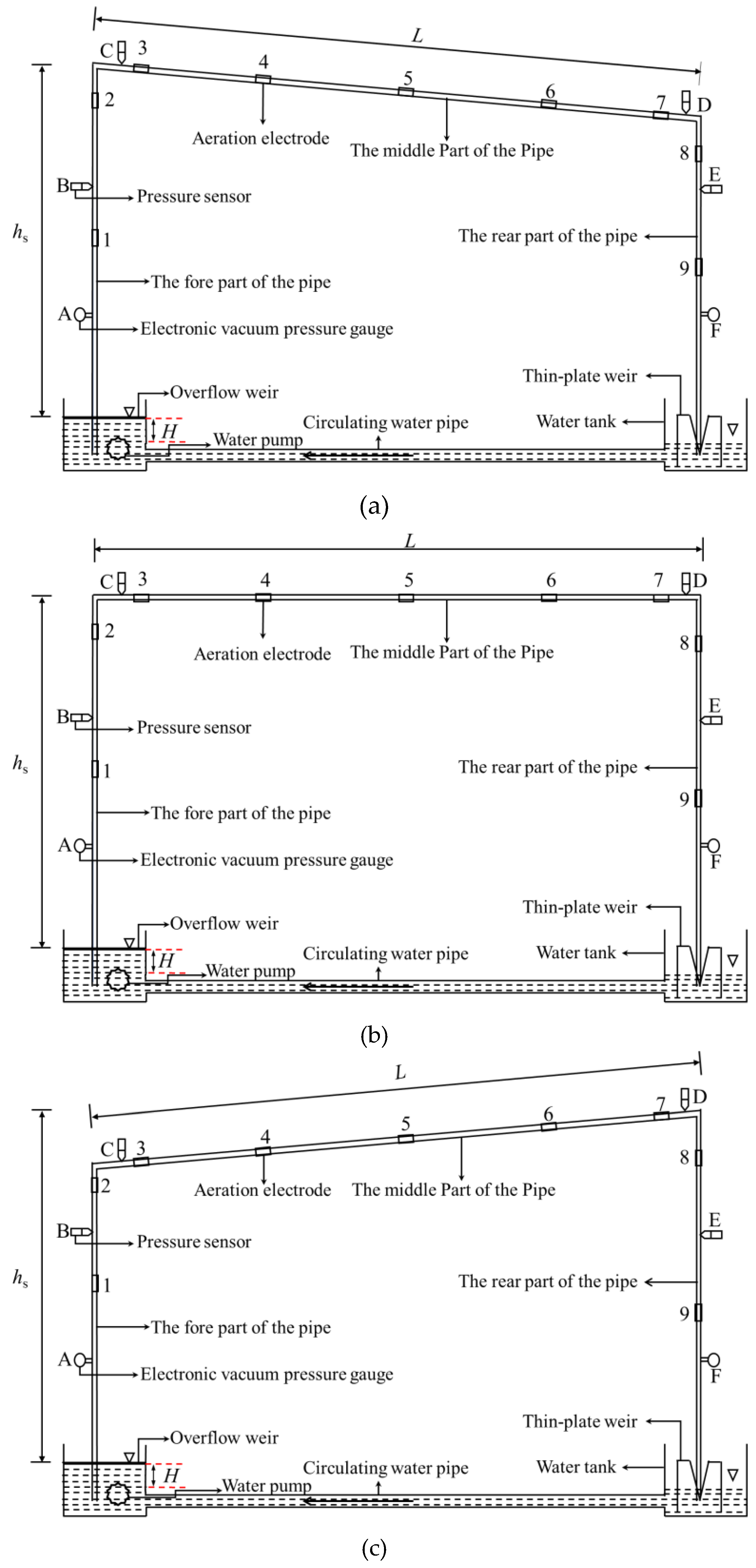
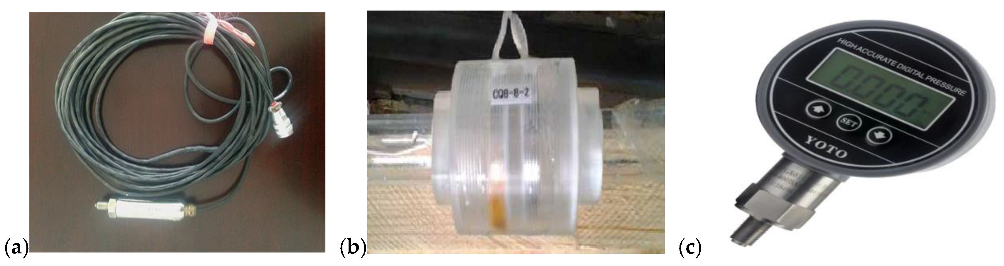
2. Materials and Methods

The test device is arranged as shown in Figure 1. The device is composed of an upstream water tank, a siphon pipeline, and a downstream water tank. The siphon pipeline is divided into the fore part, the middle part, and the rear part, all of which are made of glass tubes PMMA so as to facilitate the observation of the test phenomenon. The middle part is placed obliquely with the same length of 18.15 m under various gradients (the gradient is a negative when placed on a reverse slope and a positive on a positive slope). The following devices are arranged in sequence from upper reach to lower reach: Nine ring aeration electrodes (DDLY-2005 type with measurement accuracy of ±0.5%); four pressure sensors (KYB11G/A type with measurement accuracy of ±0.25% FS); two electronic vacuum pressure gauges (PG-801C type with measurement accuracy of ±0.20%). These devices are shown in Figure 2. The test is carried out mainly to measure the magnitude of the pressure of the siphon pipeline, gas fraction of the cross-section, and bubble velocity, etc., under various pipe diameters (2 cm, 3 cm, 6 cm), water heads (35~135 cm), and gradients (approximately ±1/60 to ±1/10) with the constant installation heights of 4 and 6 m, and to observe the gas–liquid two-phase flow in a siphon pipe under different working conditions. The pressure is measured by a pressure sensor and electronic vacuum manometer. The gas fraction of the cross-section is measured by a ring aeration electrode and conductivity meter (DDLY-2005). Finally, the flow is measured by a 20° open triangular thin-plate weir. As shown in Figure 3, the time t taken for bubbles with the same size going through a fixed distance L under different working conditions is recorded, and bubble velocity is calculated in terms of the formula v = L/t. In addition, an HDTV camera is used to record the phenomenon of gas–liquid two-phase flow under various working conditions. Problems on the prototype and model scale are not involved herein since the test is a preliminary study.

3. Results and Discussion

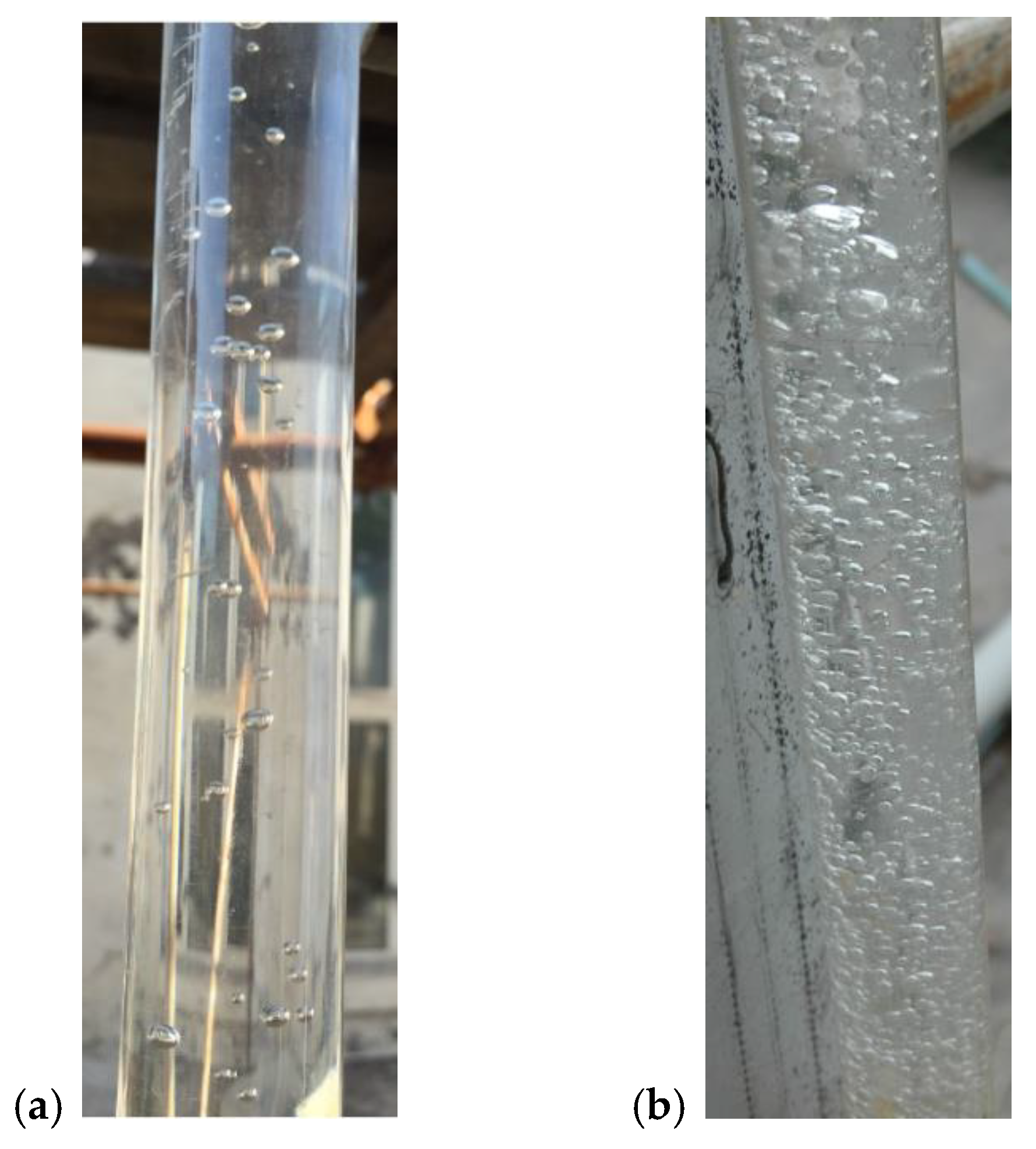
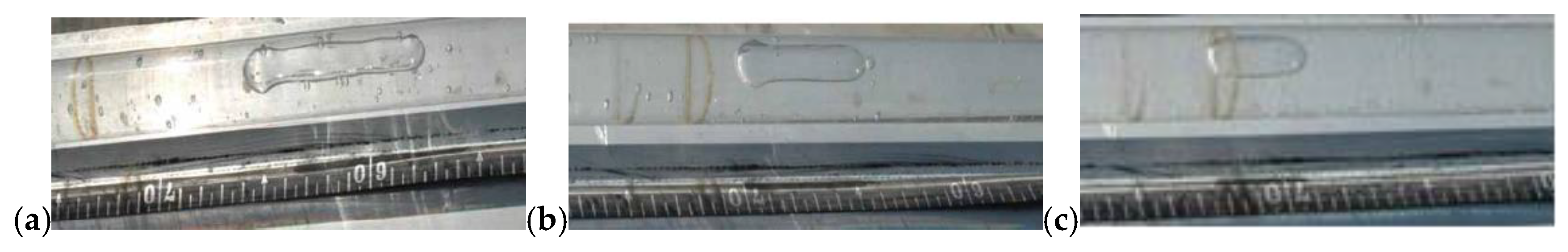
3.1. Influence of Slope on Air Mass Movement

The gas–liquid two-phase flow phenomenon in a siphon pipe under various working conditions is observed in the test, and a typical condition is selected to explain the test phenomenon. Take the 2 cm pipe with the installation height h_s = 4 m, the upstream and downstream water level H = 25 cm, and the gradient i = 0 as an example—since the installation height of the siphon pipe is high, there is a large amount of tiny bubbles in the upstream water tank which are insoluble in water and invisible to the naked eye. With the increase of the installation height, the pressure in the fore, middle, and rear parts of the pipe decrease gradually. A small amount of gas nuclei, which are invisible and insoluble in raw water, expand and separate out due to the higher pressure inside the gas nucleus as compared to that outside the gas nucleus, forming bubbles in the pipe. The flow pattern in the siphon pipeline is a gas–liquid two-phase flow. The flow state in the fore part of the siphon pipe is shown in Figure 4a. It can be seen that the bubbles in the fore part of the pipe are small in volume, and quickly flow into the middle part of the pipe after gas evolution. The water flow direction is consistent with the buoyancy direction of the bubbles, so the bubbles flow upward in the same direction as the water flow. The motion law is simple. As shown in Figure 4b, the bubbles in the rear part of the pipe flow down with water at first, and move up and down in groups after siphoning for some time. Therefore, it is difficult to measure the bubble velocity in the rear part of the pipe accurately.

Compared with the fore and rear parts, the middle part of the pipe is longer, which brings more factors influencing the bubble movement. Bubble volume, number, direction, and velocity in the pipe vary with the installation height, water head, and pipe slope. Taking h_s = 6 m and H = 35 cm as an example, Figure 5 shows the flow state in the middle part of the pipe under various gradients on the reverse slope. It can be seen that some gas pockets are attached to the pipe wall. Bubbles continuously expand by absorbing those gas pockets and flow into the rear part of the pipe at a low speed. As can be seen from the figure, if i = 0, the size of the gas pocket in the pipe is 5~6 cm, and the large gas pockets continuously absorb the bubbles attached to the pipe wall and flow into the rear part of the pipe. When the gradient increases to i = −1/60, the size of gas pockets decreases to 3~4 cm, and some 1 mm bubbles attach to the pipe wall close to the first part and do not flow with the water. When the gradient increases to i = −1/30, the size of gas pockets is about 2 cm, and the size of the bubbles attached to the pipe wall decreases. When the middle part of the pipe is fixed on the positive slope, the number and volume of bubbles in the pipe decrease with the increase of the gradient, which is consistent with the variation trend of bubbles on the reverse slope. The pseudo-cavitation phenomenon mostly occurs when the middle part of the pipe is fixed on the flat slope, and the volume of bubbles and gas pockets is larger than that on the positive or reverse slopes. For the pipes on the reverse or positive slopes, the greater the gradient, the more stable the flow state in the pipe. That is, with the increase of the gradient, the number and volume of bubbles in the middle part of the pipe decrease, the vacuum degree in the pipe decreases, the pseudo-cavitation phenomenon weakens, and the bubble velocity increases gradually.

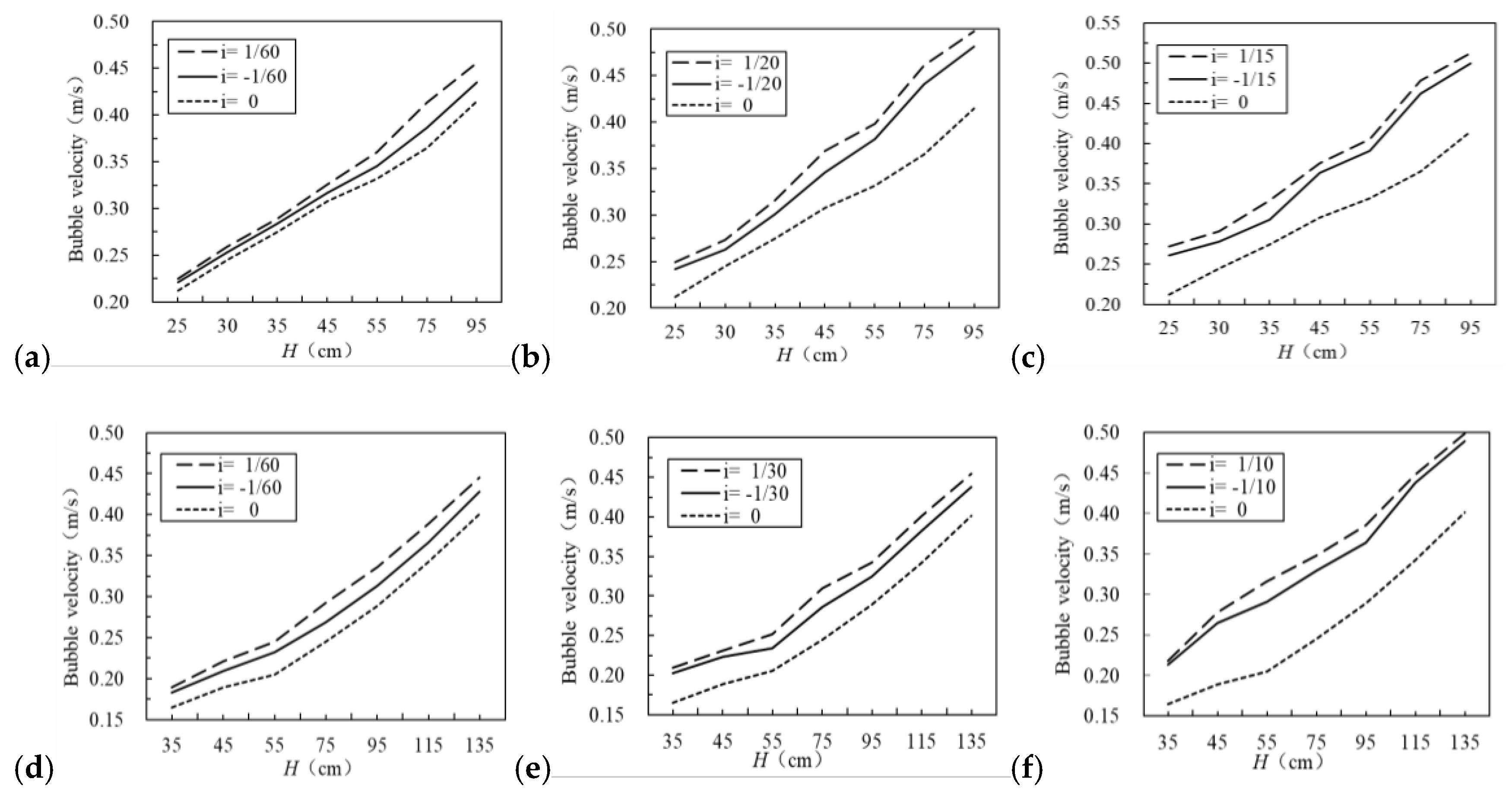
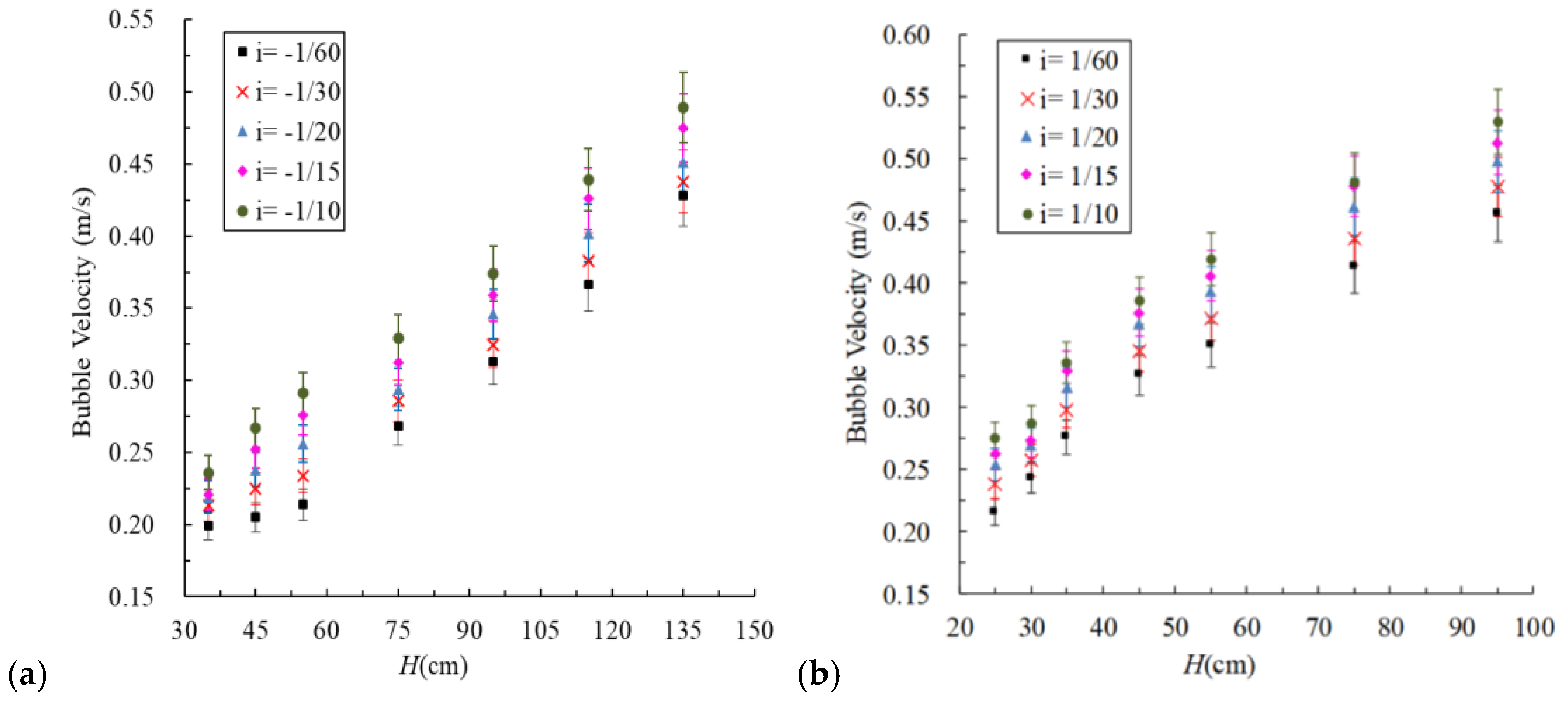
3.2. Influence of Slope on Bubble Velocity in the Pipe

Bubble velocity is calculated under various working conditions to explore the motion law of bubbles in the middle part of the pipe. When h_s = 6 m, H < 35 cm, or when h_s = 4 m, H < 25 cm (Reynolds number Re < 5000), the volume and number of bubbles in pipe are large, and the stabilization time of the siphon is short, resulting in the failure of accurate bubble velocity measurement. When h_s = 4 m, H > 95 cm (Re > 20,000), full pipe flow is nearly achieved in the pipe, and the bubbles are too tiny to measure the velocity. Therefore, the bubble movement can only be analyzed on the condition that 5000 ≤ Re ≤ 20,000. Figure 6 shows the relationship between the bubble velocity v and the water head H as well as the gradient i. According to the test data, the larger the pipe diameter, the larger the flow velocity in the pipe, and the moving speed of the bubbles is gradually increased under the drag of water. The variation of the bubble velocity is the same as that of the slope under the diameters d of 2, 3, and 6 cm; the bubble velocity in pipes of different diameters increases with increasing slope. Therefore, only the variation of bubble velocity at d = 2 cm is analyzed. It can be seen from the figure that the bubble velocity increases with the increase of the water head under a constant gradient i and installation height h_s. The bubble velocity increases with the increase of the gradient of pipes on both the reverse slope and the positive slope; that is, when the maximum vacuum degree of the middle part of the pipe remains constant, the larger the gradient of the pipe, the larger the bubble velocity. According to Figure 6a, when h_s = 4 m, H = 25 cm on the positive slope, as the gradient i increases from 1/60 to 1/10, the bubble velocity increases from 0.216 m/s to 0.275 m/s—showing an increase of 27.31%. According to Figure 6b, when h_s = 6 m, H = 55 cm on the reverse slope, the bubble velocity increases by 36.18% with the increase of the gradient. With the increase of the water head and gradient of the pipe, the flow rate of the pipe and the Re number increase. The calculation formula of the Reynolds number is shown in Formula (1). Re depends on the velocity, pipe diameter, and coefficient of kinematic viscosity. The coefficient of kinematic viscosity is related to the temperature and can be obtained by Formula (2). The water temperature of this test is controlled at 20 °C. The surface tension, viscous resistance, and buoyancy acting on the bubbles are much smaller than the inertia force, so that the bubble velocity increases under the action of inertia force.

$$Re=\frac{Vd}{\nu }$$

(1)

$$\nu =\frac{0.01775}{1+0.0377t+0.000221t^2}$$

(2)

In the above formulas, Re refers to the Reynolds number; V refers to the flow velocity (m/s); d refers to the pipe diameter (m); ν refers to the coefficient of kinematic viscosity (ν = 1.007 × 10⁻⁶ m²/s).

In order to compare the bubble velocities in the middle part of the pipe placed on the positive, flat, and reverse slopes, Figure 7 shows the relation between the bubble velocity and the flat, positive, and reverse slopes with the same gradient. Since the variation of the bubble velocity under the different pipe diameters is the same, only the bubble velocity measured with the 2 cm pipe diameter is analyzed. It can be seen from Figure 7 that the bubble velocity is at a minimum in the pipe on the flat slope under the same water head when the installation height remains constant, which is mainly because the maximum installation height—that is, the maximum vacuum degree—in the pipe remains constant as the gradient changes. When increasing the gradient of the pipe in both the positive slope and the reverse slope, the average vacuum degree in the pipe is smaller than that in the flat slope. The internal pressure of the gas nucleus remains constant while the external pressure increases, causing difficulty for gas evolution. Besides, according to the measurement results of the ring aeration electrode on the gas fraction, the gas fraction of the cross-section of the pipe placed in the positive or reverse slope is less than that in the flat slope. Under the same water head, as the actual flow area and flow capacity of the pipe increases, the inertia force acting on bubbles increases, the air carrying capacity is improved and the bubble velocity increases as well. Therefore, the bubble velocity of the middle part of the pipe on the flat slope is lower than that on the positive and reverse slopes.

It can also be seen from Figure 7 that bubbles move at a higher speed in the pipe on the positive slope than that on the reverse slope. Because the flow velocity and the Re number increase with the increase of the water head of the pipe, the inertia force acting on the gas–liquid mixture increases and the velocity difference between the water flow and bubbles decreases. The bubble velocity depends on the flow velocity, and the applied force of the water flow on the bubbles is much larger than that of buoyancy. For the pipe on the reverse slope, the component of gravity acting on the gas–liquid mixture, opposite to the inertia force, acts as a negative factor to reduce the velocity of the gas–liquid mixture. Meanwhile, for the pipe on the positive slope, the component of gravity acts in the same direction as the inertia force and thus acts as a positive force to increase its speed, so the velocity of the flow with bubbles in the pipe on the positive slope is higher than that on the reverse slope.

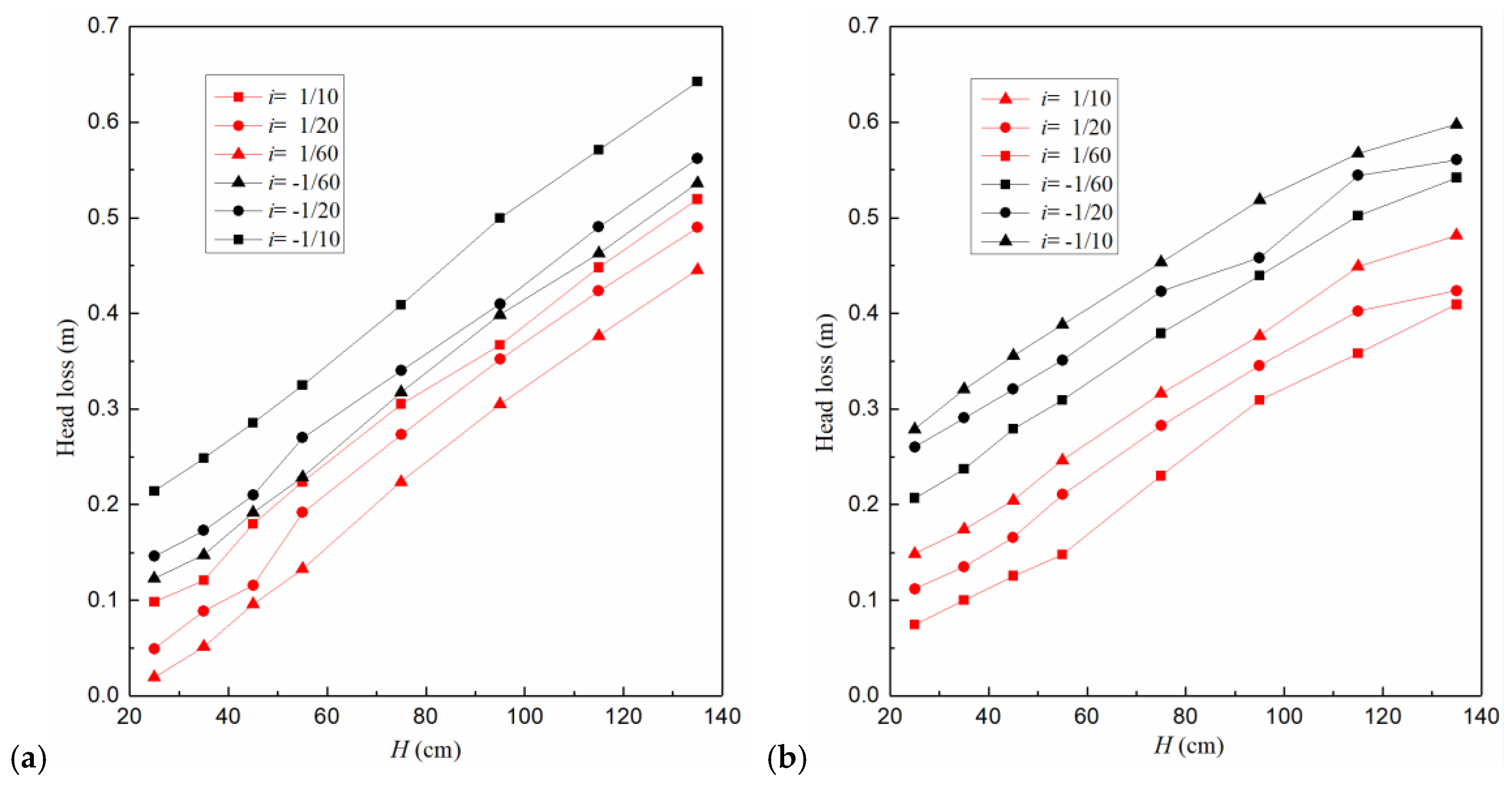
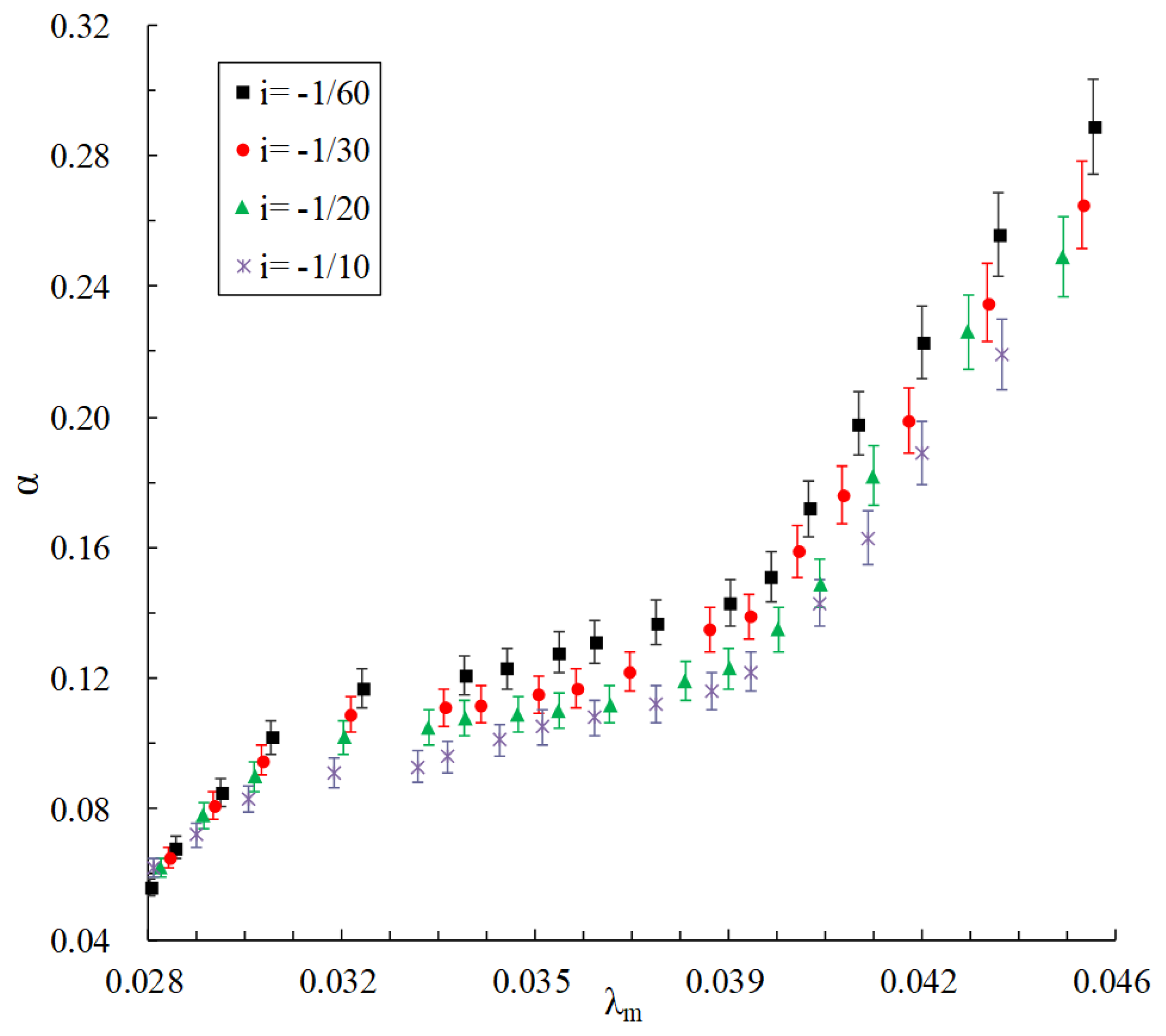
3.3. Influence of Slope on Head Loss in the Middle Part of the Pipe

In order to study the influence of slope on head loss in the siphon pipe, energy equations between the pressure sensors at the front and end of the middle part of the pipe are listed. The total head loss of the middle part of the pipe on the positive slope (h_{w P}) and reverse slope (h_{w R}) is calculated based on the measured pressure drop value of the pipe under various working conditions, as shown in Formulas (3) and (4).

$$h_{wP}=\frac{P_1-P_2}{rg}+Dh=\frac{DP}{rg}+Dh$$

(3)

$$h_{wR}=\frac{P_1-P_2}{rg}-Dh=\frac{DP}{rg}-Dh$$

(4)

In the above formulas, P₁ and P₂ respectively refer to the pressure at measuring points C, D of the electronic vacuum manometer in Figure 1, while △h refers to the water head at C, D.

Figure 8 shows the variation rule of head loss of the pipe with a diameter (d) of 3 and 6 cm with the water head and the slope at different gradient when h_s = 6 m. According to the figure, similar to common pressurized pipelines, although there is a gas–liquid two-phase flow in the pipe at different slopes, the head loss increases with the increase of the water head. Head loss increases with the increase of the gradient of the pipe with various diameters on both the positive slope and the reverse slope. When h_s and H are constant, the gas fraction of pipes on the positive slope and reverse slope decreases with the increase of the gradient. As the gas fraction decreases, the actual flow capacity in the pipe is improved and the flow velocity increases. Therefore, the greater the gradient, the greater the head loss.

It can also be seen from the figure that the head loss of the pipe on the reverse slope is significantly higher than that on the positive slope, which is obviously different from water flow in common pressurized pipelines. The head loss in common pressurized pipelines is independent of the slope. According to the measured result of the gas fraction, when h_s and H are constant, the gas fraction of the pipe on the positive slope is about 50% of that on the reverse slope. The head loss is related to not only the flow velocity but also the gas fraction. Water flow carries air mass by means of the drag force, in which process part of the water flow kinetic energy is transformed into air mass kinetic energy, causing a large head loss. In addition, the flow velocity and its inertia force increase with the increase of the water head. For the pipe on the reverse slope, the component of gravity acting on the gas–liquid mixture works opposite to the inertia force, acting as a negative force. Meanwhile, for the pipe on the positive slope, the component of gravity acts in the same direction as the inertia force, as a positive force, so the head loss in the pipe on the reverse slope is higher than that on the positive slope.

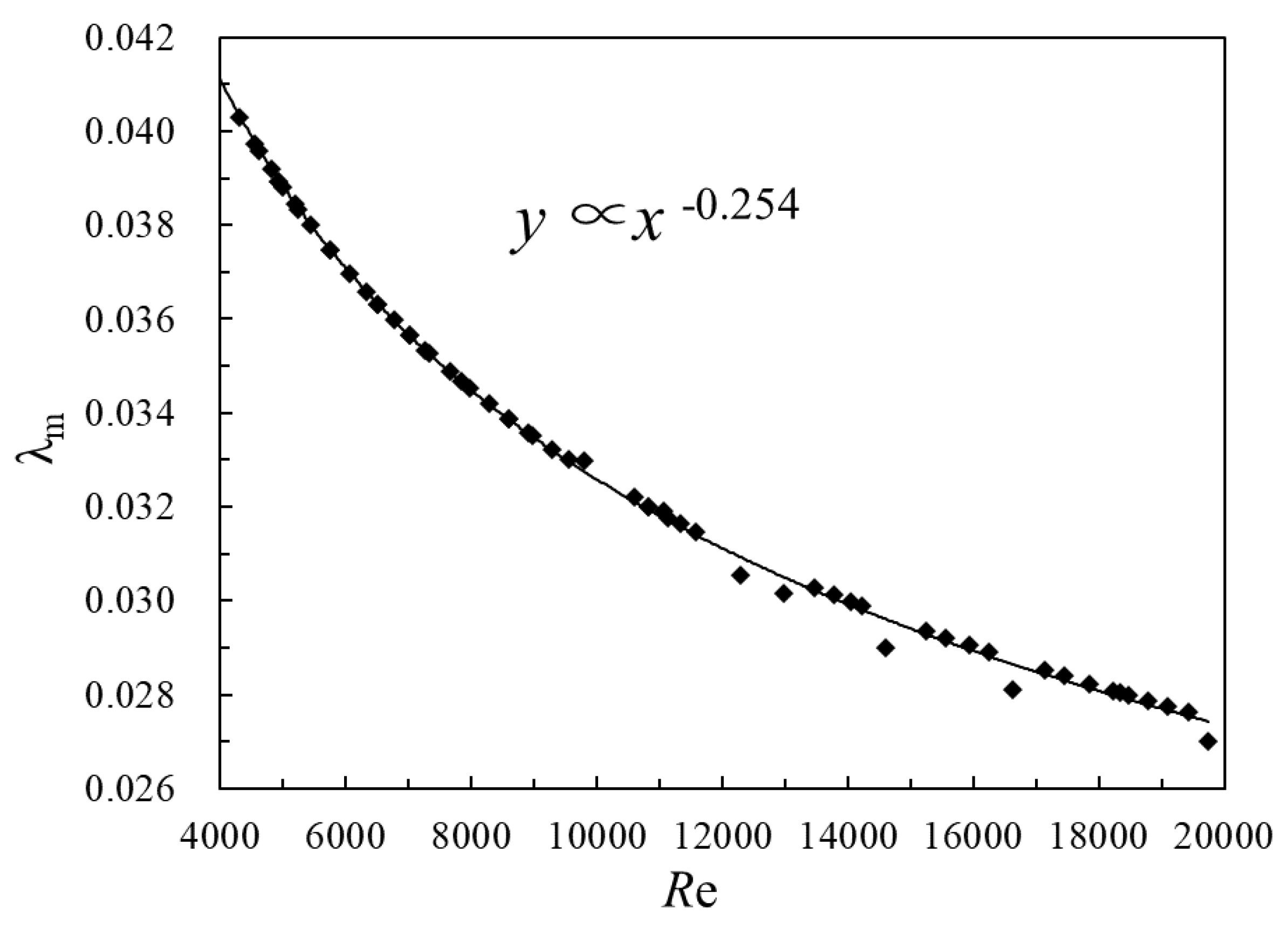
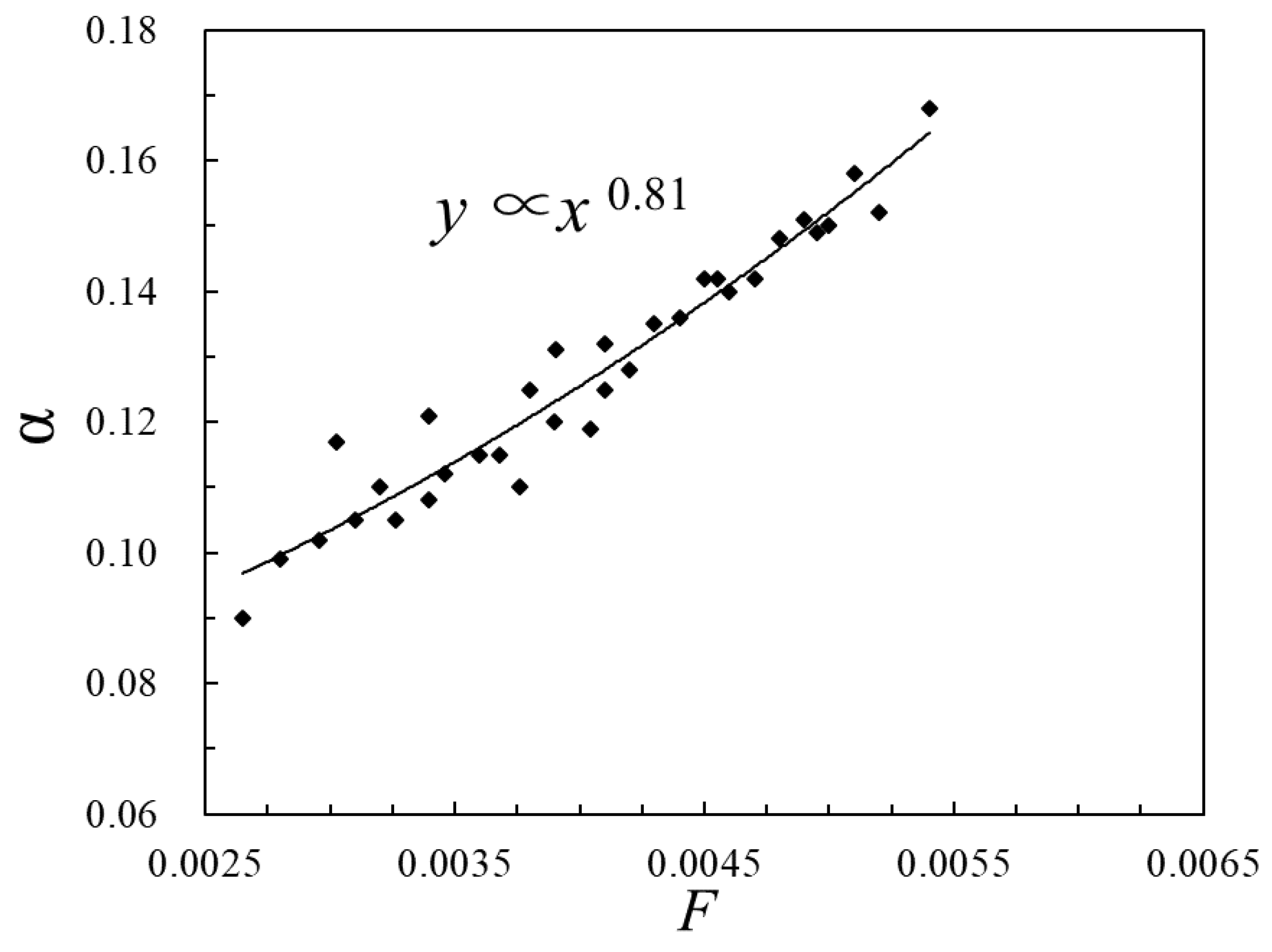
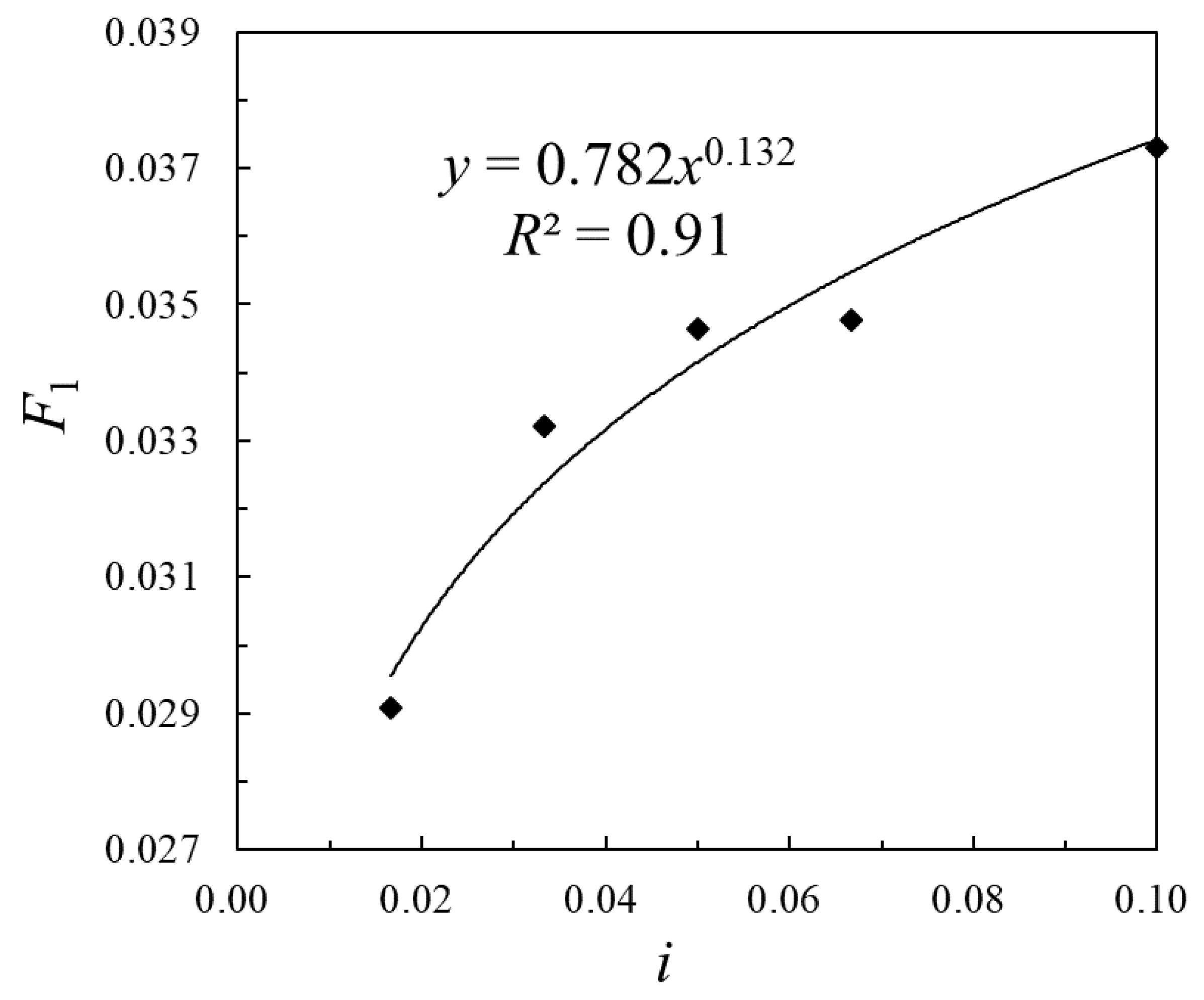
3.4. Formula Derivation and Verification of Resistance Coefficient

3.4.1. Formula Derivation of Resistance Coefficient

It is found that when Re > 5000, the gas pockets in the pipe are so tiny that the local head loss caused by the gas pockets can be ignored. The calculation formulas for the resistance coefficient (λ_m) in a siphon pipe with gas–liquid two-phase flow are shown in Formulas (5) and (6), where λ_m = f (Re, α, I, △/ d). The coefficient of absolute roughness △ in PMMA tubes with various diameters remains constant at 0.0015 mm. The formula of the resistance coefficient is deduced by the test data at d = 2 cm. When d = 2 cm, the relative roughness △/d = 0.000075, which is constant, so the influence of △/d on λ_m is not considered. This formula is also verified with test data of d = 3 and 6 cm. The resistance coefficient λ_m in the siphon pipes on the positive slope and the reverse slope with 5000 < Re < 20,000 and the gradient i of approximately ±1/60 to ±1/10 are analyzed on the basis of the test results. Figure 9 shows the relationship between λ_m and the gas fraction α under various slopes. It is found that when the gas fraction α ≤ 8%, the resistance coefficient λ_m under various gradients appears in a line, which is independent of the gradient i but related to α, that is, λ_m = f (Re, α). Bubble flow mostly appears in the pipe, occupying a small area, at which time we only need to measure the gas fraction and amend the flow sectional area in order to calculate the resistance coefficient in liquid-phase full-flow. When the gas fraction 8% < α ≤ 30%, test points corresponding to different gradients emerge in different curves, which indicates that the resistance coefficient λ_m is not only related to the gas fraction but also the gradient i, that is, λ_m = f (Re, α, i). When the maximum gas fraction is more than 30% under various working conditions, the gas pockets in the pipe rapidly gather to cut off the water flow, resulting in the failure of the remaining stable siphon. Therefore, this part focuses on the derivation of the formula of the resistance coefficient λ_m under various gradients on the positive and reverse slopes within the range of 8% < α ≤ 30%.

$$h_w\approx h_f={\lambda }_m\frac{l}{d}\frac{v^2}{2g}$$

(5)

$${\lambda }_m=h_w\frac{d}{l}\frac{2g}{v^2}$$

(6)

In the above formulas, λ_m refers to the resistance coefficient; l refers to the pipe length (m); l = 18.15 m; d refers to the pipe diameter (m); g refers to acceleration of gravity (m/s²); v refers to the flow velocity (m/s).

Taking the pipe set on the reverse slope as an example, test data at various gradients when h_s = 4 m and d = 2 cm are used to deduce the formula of the resistance coefficient λ_{m R} herein. Figure 10 shows the relationship between the resistance λ_{m R} coefficient and the Re number under various gradients. As can be seen from the figure, the resistance coefficient of the gas–liquid two-phase flow decreases with the increase of the Re number, which is consistent with the variation law of the resistance coefficient with the Re number in common pressurized pipes. λ_{m R} is in inverse proportion to the Re number under various gradients, and it is derived from data fitting that λ_{m R}∝$\frac{1}{{\mathrm{Re}}^{0.254}}$.

Set $F=\frac{l_{mR}}{\frac{1}{R{e}^{0.254}}}$. In order to further study the relationship between F and the fraction α, the values of F and α obtained under various working conditions are drawn in Figure 11. It can be seen from the figure that α ∝ F^0.881.

To further study the influence of the gradient i on λ_mR, set $\begin{array}{l}{F}_1=\frac{a}{F^{0.81}}=\frac{a}{{({\lambda }_m\times R{e}^{0.254})}^{0.81}}\end{array}$, and plot the relationship between F₁ and five different slopes i, as shown in Figure 12. Formula (7) is obtained through curve fitting:

$$F_2=0.782\times i^{0.132}$$

(7)

Formula (5) can be rewritten as the following Formula (8):

$$\frac{a}{{({\lambda }_{mR}\times R{e}^{0.254})}^{0.81}}=0.782\times i^{0.132}$$

(8)

The above formula can be simplified as:

$${\lambda }_{mR}=1.355\frac{a^{1.235}}{R{e}^{0.254}{i}^{0.163}}$$

(9)

Formula (9) is the resistance coefficient formula of the pipe on the reverse slope, where α refers to the gas fraction, Re refers to the Reynolds number, and i refers to the gradient.

According to Section 2, the variation rule of the resistance coefficient with the gradient i, the Reynolds number Re, and the gas fraction of the pipe on the positive slope is consistent with that on the reverse slope, so the derivation process of λ_m is the same on both the positive slope and the reverse slope. The resistance coefficient (λ_{m P}) formula of the pipe on the positive slope is expressed as in Formula (10).

$${\lambda }_{mP}=48.63\frac{a^{2.05}}{R{e}^{0.31}{i}^{0.59}}$$

(10)

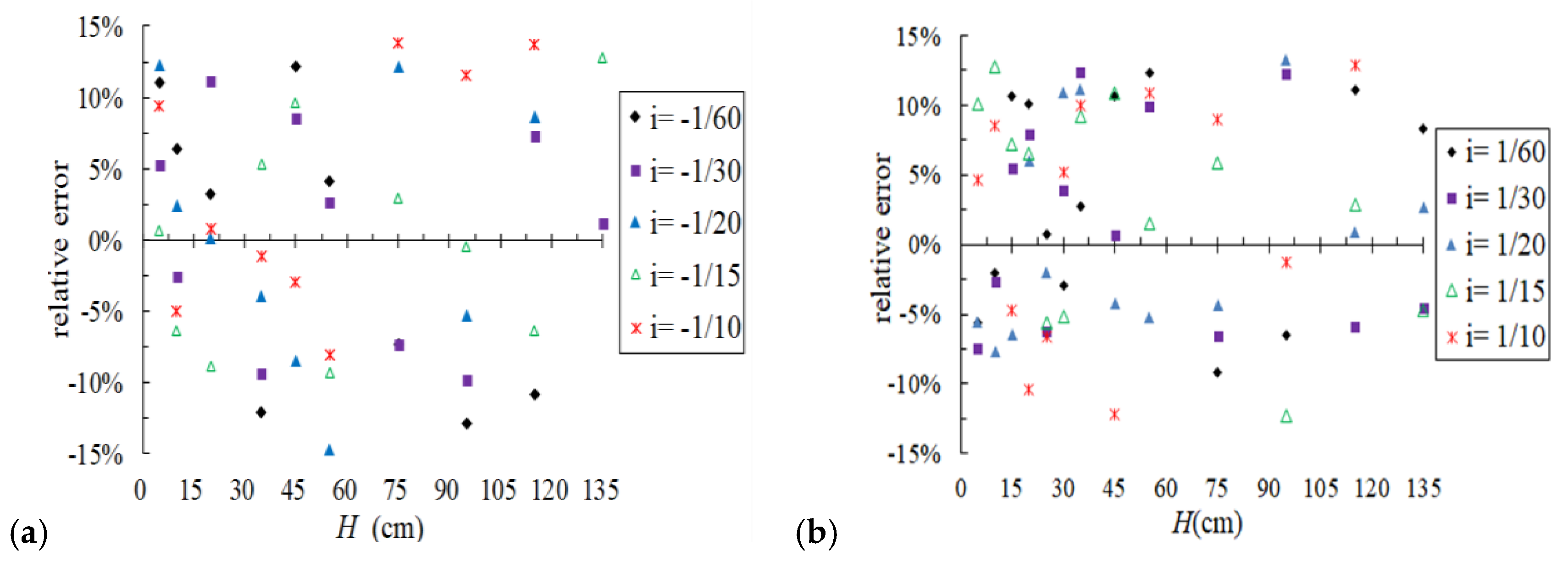
3.4.2. Verification and Error Analysis of Resistance Coefficient Formula

In order to verify the precision of the resistance coefficient formula of the pipe under various gradients on the positive slope and the reverse slope, we calculate the relative error of the measured value and the calculated value of the resistance coefficient under various gradients by Formula (11) when h_s = 6 m, and plot the relative errors of the resistance coefficient at different values of the water head in Figure 13. As can be seen from Figure 13, the maximum error of λ_{m T} and λ_m c in the reverse slope pipeline is 14.6%, and the minimum error is 0.2%. The maximum error of the positive slope pipeline is 13.2%, and the minimum error is 0.7%. The relative error of the positive slope and the reverse slope pipeline are controlled within 15%, and the error distribution is relatively uniform. It is shown that the calculation of the resistance coefficient in the siphon pipe at different slopes is suitable for Formulas (9) and (10). Since the formula deduced in this paper is an empirical formula, there are some errors between the test result and the calculated value of the formula. On the one hand, when considering the influencing factors affecting the resistance coefficient, only the main influencing factors are considered. In the determination of the variables, the parameter variables of the gas–liquid two-phase flow are neglected, resulting in defects in the formula. On the other hand, there is a certain error in the accuracy of the test instrument in the test, and there will be some error in the human reading.

$$e=\frac{{\lambda }_{\mathrm{m}\mathrm{T}}-{\lambda }_{\mathrm{m}C}}{{\lambda }_{\mathrm{m}T}}\times 100\%$$

(11)

In the above formula, e refers to the relative error value; λ_{m T} refers to the resistance coefficient in the test; λ_{m C} refers to the resistance coefficient calculated by Formulas (9) and (10).

4. Practical Implications of this Study

In this paper, the hydraulic characteristics of a gas–liquid two-phase flow under different slopes in a siphon pipe were studied through tests. Because the gas–liquid two-phase flow problem is very complicated, we encountered great challenges in our research. In the current study, it is impossible to accurately measure the temperature of the gas–liquid mixture and the presence of impurities that are invisible to the naked eye. These uncertain factors may cause deviations in the test data, and no suitable solution has yet been found to address this issue. In the general gas–liquid two-phase flow test, the gas enters the pipeline through the air compressor and then mixes with the water. The velocity of the bubbles can be accurately measured. However, in this test, the bubbles precipitated from the water body due to the pressure drop. In this test, to track the bubble motion, we measured the time required for the bubbles to pass a fixed distance and calculated the bubble velocity. There may be errors in the bubble velocity calculated in this way. The above deficiencies and challenges require the development of suitable methods to improve the accuracy of test data in future research.

Although this study deduced the formula for calculating the resistance coefficient λ_m based on test data, the theory is not perfect. Only the main factors affecting the resistance coefficient are considered in the formula. The temperature of the water–gas mixture and the mixed motion parameters of the gas–liquid two-phase are neglected. Therefore, the calculated result of λ_m may cause deviation. Due to the limited time, this paper only studies the hydraulic characteristics of the siphon pipe for the maximum installation of hs = 6 m and the maximum pipe diameter of d = 6 cm. In subsequent research, the hydraulic characteristics of the inclined siphon pipe with a larger installation height and a larger diameter should be studied. In addition, the test also found that the gathering position of the bubbles in the positive slope and the reverse slope pipeline is different. In future research, ways to set the exhaust device to increase the siphon stabilization time in the actual project and ways to lower the engineering cost should be investigated. All of the above questions need to be revised and improved in future research. Therefore, the authors will continue to study this work in the future.

5. Conclusions

The paper studied the hydraulic characteristics of a siphon pipe under different slopes. The results show that the pseudo-cavitation phenomenon in the pipe is the most serious when the middle part of the pipe is under the condition of a flat slope. When the slope is flat, the gas fraction in the pipe is greater than that of the reverse slope and the positive slope. The larger the slope is, the lower the gas fraction in the pipe. The bubble velocity increases with the increase of the slope. The bubble velocity in the flat pipe is the smallest, and the bubble velocity in the positive slope is higher than that in the reverse slope. The head loss increases with the increase of the pipe gradient in both the positive slope and the reverse slope, and the head loss in the reverse slope is greater than that in the positive slope. The resistance coefficient formula of pipes under various gradients on the positive and reverse slopes when 5000 < Re < 20,000 was obtained by means of numerical fitting. It was verified that the relative error of the formula is within 15%, indicating that the formula derived herein is applicable to the calculation of the resistance coefficient of siphon pipes under various slopes.

References

1. Liu, C.M.; Zheng, H.X. South-to-north Water Transfer Schemes for China. Int. J. Water Resour. Dev. 2002, 18, 453–471. [Google Scholar] [CrossRef]
2. Koutsoyiannis, D. Scale of water resources development and sustainability: Small is beautiful, large is great. Hydrol. Sci. J. 2011, 56, 553–575. [Google Scholar] [CrossRef]
3. Tyralis, H.; Aristoteles, T.; Delichatsiou, A.; Mamassis, N.; Koutsoyiannis, D. A perpetually interrupted interbasin water transfer as a modern Greek drama: Assessing the Acheloos to Pinios interbasin water transfer in the context of integrated water resources management. Open Water J. 2017, 4, 11. [Google Scholar]
4. Petaccia, G.; Fenocchi, A. Experimental assessment of the stage-discharge relationship of the Heyn siphons of Bric Zerbino dam. Flow Meas. Instrum. 2015, 41, 36–40. [Google Scholar] [CrossRef]
5. Tajima, N.; Sadatom, M.; Kawahara, A. Dredging of sediment in dam utilizing siphon age with sliding outer tube. Jpn. J. Multiph. Flow 2010, 241, 145–148. [Google Scholar]
6. Yan, T.; Chen, L.; Xu, M.; Zhou, M. Siphon pipeline resistance characteristic research. Procedia Eng. 2012, 28, 99–104. [Google Scholar]
7. Seo, K.; Kang, S.H.; Kim, J.M.; Lee, K.Y.; Jeong, N.; Chi, D.Y.; Yoon, J.; Kim, M.H. Experimental and numerical study for a siphon breaker design of a research reactor. Ann. Nucl. Energy 2012, 50, 94–102. [Google Scholar] [CrossRef]
8. Kang, S.H.; Ahn, H.S.; Kim, J.M.; Joo, H.M.; Lee, K.Y.; Seo, K.; Chi, D.Y.; Yoon, J.; Jeun, G.D.; Kim, M.H. Experimental study of siphon breaking phenomenon in the real-scaled research reactor pool. Nucl. Eng. Des. 2013, 255, 28–37. [Google Scholar] [CrossRef]
9. Kang, S.H.; Lee, K.; Lee, G.C. Investigation on effects of enlarged pipe rupture size and air penetration timing in real-scale experiment of siphon breaker. Nucl. Eng. Technol. 2014, 46, 817–824. [Google Scholar] [CrossRef]
10. Matozinhos, C.F.; Santos, A.A.C. Two-phase CFD simulation of research reactor siphon breakers: A verification, validation and applicability study. Nucl. Eng. Des. 2018, 326, 7–16. [Google Scholar] [CrossRef]
11. Jin, S.F.; Liu, H.X.; Ding, W.; Shang, H.; Wang, G.L. Sensitivity Analysis for the Inverted Siphon in a Long-Distance Water Transfer Project: An Integrated System Modeling Perspective. Water 2018, 10, 292. [Google Scholar] [CrossRef]
12. Diogo, A.F.; Oliveira, M.C. A simplified approach for the computation of steady two-phase flow in inverted siphons. J. Environ. Manag. 2016, 166, 294–308. [Google Scholar] [CrossRef] [PubMed]
13. Revellin, R.; Thome, J.R. A theoretical motel for the prediction of the critical heat flux in heated micro channels. Int. J. Heat Mass Trans. 2008, 51, 1216–1225. [Google Scholar] [CrossRef]
14. Chorai, S.; Nigam, K.D.P. CFD modeling of flow profiles and interfacial phenomena in two-phase flow in pipes. Chem. Eng. Process. 2006, 45, 55–65. [Google Scholar]
15. Musa, A.; Danjuma, Y.; Lao, L.Y. Interfacial friction in upward annular gas-liquid two-phase flow in pipes. Exp. Therm. Fluid Sci. 2017, 84, 90–109. [Google Scholar]
16. Shams, R.; Tavakoli, A. Experimental investigation of two-phase flow in horizontal wells: Flow regime assessment and pressure drop analysis. Exp. Therm. Fluid Sci. 2017, 88, 55–64. [Google Scholar] [CrossRef]
17. Schmidt, J.; Claramunt, S. Sizing of rupture disks for two-phase gas/liquid flow according to HNE-CSE-model. J. Loss Prev. Process Ind. 2016, 41, 419–432. [Google Scholar] [CrossRef]
18. Chen, F.; Sun, B.; Wang, E.P. Research on the dynamic characteristics of gas-liquid two phase flow measurement with different throttle devices. J. Exp. Fluid Mech. 2012, 26, 55–60. [Google Scholar]
19. Pietrzak, M.; Placzek, M.; Witczak, S. Upward flow of air-oil-water mixture in vertical pipe. Exp. Thermal Fluid Sci. 2017, 81, 175–186. [Google Scholar] [CrossRef]
20. Kjeldby, T.K.; Nydal, O.J. A Lagrangian three-phase slug tracking framework. Int. J. Multiph. Flow 2013, 56, 184–194. [Google Scholar] [CrossRef]
21. Wang, Q.; Polansky, J.; Karki, B.; Wang, M.; Wei, K.; Qiu, C.; Kenbar, A.; Millington, D. Experimental tomographic methods for analyzing flow dynamics of gas-oil-water flows in horizontal pipeline. J. Hydrodyn. 2016, 28, 1018–1021. [Google Scholar] [CrossRef]
22. Barnea, D.; Shoham, D. Flow pattern transitions for gas-liquid flow in horizontal and inclined pipes: Comparison of experimental data with theory. Int. J. Multiph. Flow 1980, 6, 217–225. [Google Scholar] [CrossRef]
23. Wiesman, J.; Kang, S.Y. Flow pattern transition in vertical and upwardly inclined lines. Int. J. Multiph. Flow 1981, 7, 271–291. [Google Scholar] [CrossRef]
24. Barnea, D.A.; Shohamo, O.; Tatel, Y. Gas-liquid flow in inclined tubes: Flow pattern transitions for upward flow. Chem. Eng. Sci. 1985, 40, 131–136. [Google Scholar] [CrossRef]
25. Barnea, D. A unified model for predicting flow-pattern transition for whole ranges of pipe inclinations. Int. J. Multiph. Flow 1987, 13, 1–12. [Google Scholar] [CrossRef]
26. Pansunee, S.; Somchai, W. An experimental study of two-phase air-water flow and heat transfer characteristics of segmented flow in a microchannel. Exp. Therm. Fluid Sci. 2015, 62, 29–39. [Google Scholar]
27. Kawahara, A.; Mohamed, H.M.; Sadatomi, M.; Law, W.Z.; Kurihara, H.; Kusumaningsih, H. Characteristics of gas-liquid two-phase flows through a sudden contraction in rectangular microchannels. Exp. Therm. Fluid Sci. 2015, 66, 243–253. [Google Scholar] [CrossRef]
28. Chiwoong, C.; Moohwan, K. Flow pattern-based correlations of two-phase pressure drop in rectangular microchannels. Int. J. Heat Fluid Flow 2011, 32, 1199–1207. [Google Scholar]
29. Bhagwat, S.M.; Ghajar, A.J. Experimental Investigation of Non-Boiling Gas-Liquid Two Phase Flow in Downward Inclined Pipes. Exp. Therm. Fluid Sci. 2017, 89, 219–237. [Google Scholar] [CrossRef]
30. Schubert, D.; Costello, P.; Heintzman, T.; Lohr, E. Vacuum sewer design construction and operation in rural Alaska. In On-Site Wastewater Treatment, Proceedings of the Ninth National Symposium on Individual and Small Community Sewage Systems, Fort Worth, TX, USA, 11–14 March 2001; ASAE: Washington, DC, USA, 2001; pp. 369–376. [Google Scholar]
31. Anonymous. Vacuum Sewers Help Clean Up Michigan Lakes. Water Environ. Technol. 2004, 16, 102. [Google Scholar]
32. Anonymous. High water table/flat terrain a climate for vacuum sewer system. Public Works 2002, 133, 36–38. [Google Scholar]
33. Mandal, A.; Kundu, G.; Mukherjee, D. Studies on frictional pressure drop of gas-non-Newtonian two-phase flow in a cocurrent downflow bubble column. Chem. Eng. Sci. 2004, 59, 3807–3815. [Google Scholar] [CrossRef]
34. Donald, D.; Gray, P.E. Design Programs for Vacuum Sewer System. Ph.D. Thesis, Department of Civil. Engineering West. Virginia University, Charlottesville, VA, USA, 1990; pp. 182–189. [Google Scholar]
35. U.S. Environmental Protection Agency. Manual Alternative Wastewater Collection Systems; EPA: Washington, DC, USA, 1991; pp. 35–93.
36. Duan, J.M.; Zhou, J.X. Studies on Frictional Pressure Drop of Gas-non-Newtonian Fluid Two-phase Flow in the Vacuum Sewers. Civ. Eng. Environ. Syst. 2006, 23, 1–10. [Google Scholar]
Figure 1. Layout of test devices: (a) pipeline on the positive slope, (b) pipeline on the flat slope, (c) pipeline on the reverse slope.
Note: 1–9 refer to aeration electrodes; A, F refer to electronic vacuum pressure gauges; B, C, D, E refer to pressure sensors; L refers to the length of the middle part of the siphon pipe (m); hs refers to the installation height (m).
Water 11 01095 g001
Figure 2. Pressure sensor and electronic vacuum manometer: (a) pressure sensor, (b) aeration electrode, (c) electronic vacuum pressure gauge.
Water 11 01095 g002
Figure 3. Measurement of the bubble velocity.
Water 11 01095 g003
Figure 4. Flow state distribution in the fore and rear parts of the siphon pipe: (a) the fore part of the pipe, (b) the rear part of the pipe.
Water 11 01095 g004
Figure 5. Flow state in the middle part of the pipe under various gradients: (a) i = 0, (b) i = −1/60, (c) i = −1/30.
Water 11 01095 g005
Figure 6. Relationship between the bubble velocity and water head, gradient: (a) hs = 4 m, (b) hs = 6 m.
Water 11 01095 g006
Figure 7. Comparison of the bubble velocity in the middle part of pipe on the positive, flat, and reverse slopes: (a) hs = 4 m and i = ±1/60, (b) hs = 4 m and i = ±1/20, (c) hs = 4 m and i = ±1/15, (d) hs = 6 m and i = ±1/60, (e) hs = 6 m and i = ±1/30, (f) hs = 6 m and i = ±1/10.
Water 11 01095 g007
Figure 8. Variation of the head loss hw with water head under various slopes, hs = 6 m: (a) d = 3 cm, (b) d = 6 cm.
Water 11 01095 g008
Figure 9. Relationship between the resistance coefficient λm and gas fraction under various gradients.
Water 11 01095 g009
Figure 10. Relationship between the Re number and the resistance coefficient λm R.
Water 11 01095 g010
Figure 11. Relationship between F and the gas fraction α.
Water 11 01095 g011
Figure 12. Relationship between the gradient i and F1.
Water 11 01095 g012
Figure 13. Relative error between the test value and the calculated value of the resistance coefficient: (a) pipes set on the reverse slope, (b) pipes set on the positive slope.
Water 11 01095 g013