Article

Probability Analysis and Control of River Runoff–sediment Characteristics based on Pair-Copula Functions: The Case of the Weihe River and Jinghe River

1
School of Environmental Science and Engineering, Chang’an University, 126 Yanta Road, Xi’an 710054, China
2
College of Science, Chang’an University, Xi’an 710064, China
3
Key Laboratory of Subsurface Hydrology and Ecological Effects in Arid Ministry of Education, Chang’an University, 126 Yanta Road, Xi’an 710054, China
4
Institute of Water and Development, Chang’an University, 126 Yanta Road, Xi’an 710054, China
5
Xi’an Institute of Optics and Precision Mechanics of Cas, Xi’an 710070, China
*
Author to whom correspondence should be addressed.
Water 2019, 11(3), 510; https://doi.org/10.3390/w11030510
Submission received: 25 December 2018 / Revised: 7 March 2019 / Accepted: 7 March 2019 / Published: 12 March 2019
(This article belongs to the Section Hydrology)

Abstract

:
Analyzing the encounter frequency of high–low runoff and sediment yield is important for the appropriate dispatching of runoff–sediment resources, as well as river regulation. However, there have been no reports on the utilization of the pair-copula function in analyzing the runoff–sediment characteristics from a probabilistic perspective and conducting probability control on the runoff–sediment yields of different hydrologic stations. This paper builds marginal distribution functions on the basis of kernel distribution theory. In addition, this paper builds the joint distribution functions through pair-copula functions in order to analyze the encounter probability and the compensation characteristics of high–low runoff and sediment at different stations on the Weihe River in China, as well as the origins of runoff–sediment, to conduct probability control of river runoff–sediment resource allocation. The results show that, in different periods, the synchronous probability of high–low runoff of the Weihe River’s Xianyang and Huaxian Stations, and the Jinghe River’s Zhangjiashan Station differ, while that of high–low sediment at the three stations changes little—remaining at around 54%. Therefore, the sediment and runoff of the Weihe River apparently have different origins. In years of high and low runoff, if the runoffs of the Xianyang and Zhangjiashan Stations can be kept within a certain range, then the runoff of the Huaxian Station will be in a particular range, at a certain probability. Sediment at the Huaxian Station can be controlled, in a similar way. These results are of great significance for the water and sediment management department of the Weihe river, in order to reasonably allocate water and sediment resources.

1. Introduction

Learning the characteristics of runoff–sediment migration and analyzing the encounter frequency of high–low runoff–sediment of rivers will provide a theoretical basis for the development and control of runoff–sediment resources. Thus, the key to analyzing the encounter probability of high–low runoff–sediment is to establish the joint distribution function with several hydrological variables. Presently, the study of the hydrological distribution function of two variables is relatively mature. However, the establishment of three- and higher-dimensional joint distribution functions of multi-variables still need exploring [1]. Major research methods of calculating the hydrological frequency with multi-variables include the normal distribution and normal transformation method, the same marginal distribution construction method, the non-parametric estimation method, the multi-to-one-dimension transformation method, and the empirical frequency method. However, some of these methods require harsh assumptions, some of them are complicated to calculate, and some are difficult to extend [1,2,3,4].
The copula function, however, is flexible to adapt. It does not require the same distribution for marginal distributions, and its solution is quite simple. The copula function was first applied to the hydrological field in 2003 [5] and is now applied widely to the hydrological field. Major research results include: De Michele (2005) used the 2D copula function to calculate the designed flood yield of dams, and Salvadori (2006) used the 2D copula function to study the statistical characteristics of storms at sea [6,7]. De Michele (2013) and Linlin (2018) applied copula functions to analyze the drought frequency and its recurrence interval [8,9]. Razmkhah (2016) [10] and Yan (2018) [11] used the 2D copula function to study the relationship between precipitation and runoff. Recently, 3D and higher-dimensional copula functions have also been applied. For example, Liu (2015), Pham (2016), and Gyasi-Agyei (2012) [12,13,14] analyzed precipitation characteristics through the 3D copula function. Ridolfi (2013) [15] evaluated levels of precipitation through the 3D copula function. Graele (2013) [16] estimated the designed water level through the 3D copula function. Wahl (2012) [17] utilized the 3D copula function to analyze hydrodynamic boundary conditions in coastal areas. So far, analysis of encounter frequencies of high–low runoff–sediment mainly adopts 2D copula functions, which are obviously incapable of satisfying practical needs. Additionally, some scholars analyzed the encounter frequency of the high–low runoff–sediment of several variables through 3D-symmetric copula and non-symmetric 3D and 4D copula of particular structures [17,18], but the particular structures were limited, to some extent, and their parameters were, at times, complicated for finding the solution. The study of using copula functions to analyze the relationship between runoff and sediment is given in [19]. Empirical formulae and other deterministic methods were also used in the study of the runoff–sediment relationship [20], but these deterministic methods ignored the randomness of the variables. At present, methods of runoff and sediment regulation include genetic algorithms [21], dynamic programming methods [22], multi-objective optimization algorithms [23], and so on, but, sometimes, it is difficult to find the optimal solution of these methods. However, there have been few studies using the copula function to analyze the control of runoff and sediment.
The pair-copula function is a relatively flexible method in building high-dimensional copula functions, and its parameters are relatively simple to solve. While dealing with the joint probability, we don’t need to consider whether the marginal distributions are the same, or the positive and negative correlation between the variables [24]. Besides, multidimensional density functions can be decomposed into several pair-copula functions in order to solve, decreasing the complexity of the multidimensional joint probability distribution structure. Huaxiong (2014) used the vine-copula pair-copula function to analyze the relationships among annual precipitation, annual evaporation capacity, and annual runoff [25]. Vernieuwe (2015) [26] and Callau Poduje (2018) [27] analyzed precipitation frequency through the vine-copula function. Shafaei (2017) analyzed flood frequency by vine-copula [28]. However, analysis on the encounter frequencies of high–low sediment at different river stations in compensation relationships, and research on probability control of the runoff–sediment yield of different stations through pair-copula functions has not been carried out, yet.
Being the major tributary to the Yellow River, the Weihe River is regarded as the mother river of Gansu and Shaanxi Provinces. It is the primary water supply for 29.5 million people living in Shaanxi and Gansu Provinces, and in the Ningxia Hui Autonomous Region. Among numerous tributaries to the Weihe River, the Jinghe River is the largest. Throughout history, the Weihe River has flooded several times, and its downstream channels have often been congested due to sediment accumulation, bringing huge economic losses to its bank areas. Recently, however, runoff–sediment yields of the Weihe River have reduced sharply, worsening the trend of drought. As the social economy boosts, the utilization range and amount of runoff–sediment resources of the Weihe River also vary. The key problem that the runoff–sediment resources dispatching department deals with is how to dispatch and allocate the runoff–sediment resources of the upper and lower reaches of the Weihe River, reasonably. Therefore, it is necessary to analyze the runoff–sediment characteristics of the Weihe River. Throughout the years, scholars have studied the runoff–sediment characteristics of the Weihe and Jinghe Rivers, respectively, from different perspectives [29,30,31,32,33].
This paper’s novelty is in adopting a pair-copula function to analyze the encounter frequency of high–low annual runoff–sediment yields between different stations, which have a direct compensation relationship, from a probabilistic perspective. Furthermore, the pair-copula function is used to explore the origins of the runoff and sediment of the river, and to conduct probability control on the downstream runoff and sediment yield. The major contributions of this paper include: (1) Analyzing the 1960–2016 variation tendencies and sudden mutations of annual runoff and sediment yield of the three hydrologic stations, on the basis of the RAPS (Rescaled Adjusted Partial Sums) method; (2) Building the marginal distribution function of the annual runoff and sediment yield of each observation station through the kernel distribution method; (3) Establishing the 3D copula function of annual sediment yield and annual runoff yield of the three stations through a pair-copula function; (4) Analyzing the encounter frequency of high–low runoff–sediment of the Weihe River Huaxian and Xianyang Stations, and the branching Jinghe River Zhangjiashan Station, from a probabilistic perspective; (5) Respectively analyzing the probability relationships of runoff and sediment yields between the downstream Huaxian and Xianyang Stations, and the branching Zhangjiashan Station, through conditional probability formulas; and (6) Estimating the designed runoff and sediment yields of upstream stations, both in high and low runoff years, which can guarantee the runoff and sediment yields of downstream stations in a particular range at a certain probability.

2. Materials and Methods

2.1. Research Area and Data

2.1.1. Brief Introduction to the Research Area

The Weihe River (104–110° E, 33–37° N) originates in the Niaoshu Mountains of Weiyuan County, Gansu Province and mainly flows through Tianshui of Gansu Province and Baoji, Xianyang, Xi’an, Weinan, and so on, of the Guanzhong Plain, Shaanxi Province. It joins the Yellow River in the Tongguan County, Weinan City (Figure 1). The Weihe River is the largest tributary to the Yellow River, covering a basin area of 134,800 km2. Its total length reaches 818 km. The upper reaches of the Weihe River start at Weiyuan and end at the exit of the Baoji Canyon; the middle reaches start at the Baoji Canyon and end at Xianyang; and the lower reaches of the river are from Xianyang to the Tongguan river estuary. Huaxian Station is the mouth where the Weihe River joins the Yellow River. Four seasons are distinct in the Weihe River basin, and precipitation is not uniformly distributed in the area. It is dry, with little rain, in the winter, with heavy rains in the summer. In this area, the average annual precipitation is 572 mm; however, more than 60% of the annual rainfall is from July to October. The rainfall is scarce in January and December, much less than 1% of the annual precipitation. At Xianyang Station, the annual average runoff is 36.8 × 10⁸ m3 (1960–2016), and the annual sediment runoff is 0.88 × 10⁸ t (1960–2016). As for flood season, water and sediment over the whole year take up 59% and 85%, respectively. Downstream at the Huaxian Station, the annual average runoff is 63.4 × 10⁸ m3 (1960–2016), and average sediment is 2.73 × 10⁸ t (1960–2016); runoff and sediment in flood season (from July to October) cover 60% and 89% or so, respectively, for the whole year. Mountainous areas of the WRB (Weihe River basin) mark 84% of the total area of the WRB, which is composed of plateau mountains and plain mountains. Plateau mountains of the WRB are mainly located in basins of the Jinghe and upper Weihe Rivers. The topographic feature of WRB is “west high, east low”, where the highest altitude in the west reaches 3495 m. From the west to the east, the terrain gradually becomes lower and the river valley wider. The climate in the WRB is a warm-temperate, semi-wet, and semi-arid monsoon climate, with characteristics of a mountain basin climate. The average temperature of WRB in a year is 12.8 °C [19].
The Jinghe River (106° E to 109° E, 34° N to 37° N) is the largest tributary to the Weihe River. It originates in the east side of the Liupanshan Mountain, in Southeastern Weibaliang, Jingyuan County, in the Ningxia Hui Autonomous Region. The total length of Jinghe River reaches 455.1 km, covering a basin area of 45,400 km2, which is 33.7% of the WRB. The Jinghe River flows through the Ningxia Hui Autonomous Region, as well as the Gansu and Shaanxi Provinces, and meets the Weihe River in the Gaoling District, Xi’an City, Shaanxi Province. The topographic feature of the Jinghe River Basin (JRB) is “northwest high, southeast low”. With very sparse vegetation (only making 10% of the total area), soil erosion in the JRB area is severe, making it the main sediment source of the Weihe River. Hydrologic stations of the Jinghe River are illustrated in Figure 1.

2.1.2. Data

The study collected the data of annual runoff and sediment yield from 3 hydrometric stations: The Huaxian and Xianyang Stations of the Weihe River, and the Zhangjiashan Station (Figure 1) of its biggest branch, the Jinghe River, over 57 years (1960–2016). Among these, the runoff data were recalculated by the measured flow data of the hydrological stations, with the observing frequency being once every day, and the frequency was increased, based on the actual requirement (especially in flood season). In this paper, the sediment yield was obtained by recalculating the index sediment concentration, which refers to the average sediment concentration for one or several representative vertical lines at the cross-section. Based on the measured samples at 3 hydrological stations for many years, the correlation curve was drawn for every station, reflecting the index sediment concentration and the average sediment concentration at the cross-section; the former was shown on the vertical coordinate, and a horizontal coordinate indicated the latter. Because the correlation of the sediment concentration and the average sediment concentration at the cross-section are very good, the average sediment concentration at the cross-section was derived by the index sediment concentration and the relation between it and the average sediment concentration at the cross-section. After that, the sediment discharge could be acquired by the average sediment concentration at the cross-section and the average flow at the cross-section. The vertical mixing method was mainly adopted for sampling the index sediment concentration. Firstly, on the relevant observation points of the vertical lines, we took the sampling respectively and mixed them into one sample, the sediment concentration of which was taken as the average for the line. The relative water depths (the ratio between the underwater penetration of instrument and water depth) of the points on the line are 0.2, 0.6 and 0.8; 0.2 and 0.8 assuming that there were two points; and 0.5 for one point. The mixing method of samples on the same vertical line was to mix multiple samples into one sample in a certain proportion. Mixing at a ratio of 2:1:1 assuming that there were 3 points, 1:1 if there were 2 points. The number for the lines and the points was determined in accordance with river bed characteristics and water and sediment conditions. Sampling frequency was several times within one day during flooding, once a day during normal river flow periods and once within 2 to 3 days in dry season. Daily sediment discharge at the cross-section was calculated as follows: (1) Supposing that the index sediment concentration was taken several times within a day, the flow weighting method was applied for calculating daily average sediment discharge, and the formula was shown as follows: Within Q S ¯ = i = 1 n [ ( q i C s i + q i + 1 C s ( i + 1 ) ) Δ t i ] , Q S ¯ represented daily average sediment discharge in kg/s; q i was the average flow at the cross-section when it was at i, indicated by m3/s; C s i was the average sediment concentration in kg/m3 at the cross-section when it was at i. Δ t i was in h, showing the time interval between C s i and C s ( i + 1 ) ; n was the times for measuring the index within a day. (2) In cases where the index sediment concentration was obtained only once a day, we took the average sediment concentration of the cross-section derived from the index sediment concentration as the daily average sediment concentration of the cross-section, then multiplied it by the daily average river flow, and the daily average discharge could be received for the day; (3) when taking the index sediment concentration once every few days, and the index sediment concentration was not measured, the average sediment concentration of the cross-section for each different day was acquired by straight-line interpolation for the cross-section sediment concentration before and after the index sediment concentration had been measured; after that, we multiplied it by the average river flow of each different day, and the daily average sediment discharge for each day was obtained. The formula for calculating annual sediment discharge in this paper was W s = ( 86400 i = 1 m Q s ¯ ) / 10 11 , and in it, W s was the annual discharge in 108 t, there were 86,400 s for a day, and m was the days of a year. The aforementioned data were provided by the Shaanxi Provincial River Reservoir Administration. The data were strictly controlled in quality before release, since the Bureau was authorized for data statistics, publishing for all the rivers and reservoirs in the province.

2.2. Research Methods

2.2.1. Rescaled Adjusted Partial Sums (RAPS) Method

RAPS is used to standardize, and then study, time series data. This method could be applied to the study of variation of the trend of time series data, to find the inflection points of the trend. The advantage of the method is to avoid the impacts of different data units and random errors on analysis. Formula of RAPS is expressed, as follows:
RAPS k = t = 1 k y t y ¯ s y .
In the formula, k represents the number of observation data, y t represents the parameter observed at time t, y ¯ represents the average value of the parameter sequence observed, and s y represents the standard deviation [34].

2.2.2. Pair-Copula Function

Suppose that X = ( X 1 , X 2 , , X n ) is the n-dimensional vector in accordance with the joint density function f ( x 1 , x 2 , , x n ) . Then, its marginal density function is f i ( x i ) , ( i = 1 , 2 , , n ) , and it can be inferred, in accordance with the conditional probability, that:
f ( x 1 , x 2 , , x n ) = f n ( x n ) · f n 1 | n ( x n 1 | x n ) · f n 2 | n 1 , n ( x n 2 | x n 1 , x n ) · f 1 | 2 , , n ( x 1 | x 2 , , x n ) .
According to Sklar’s Theorem [35], the multivariate joint distribution function can be described, through the copula function and the marginal distribution function; that is:
F ( x 1 , x 2 , , x n ) = C 1 , 2 , , n [ F 1 ( x 1 ) , F 2 ( x 2 ) , , F n ( x n ) ] .
In the formula, C 1 , 2 , , n ( · ) represents the distribution function of an n-dimensional copula function, and F i ( x i ) ,   ( i = 1 , 2 , , n ) is the marginal distribution function.
Therefore, the joint density function can be described as:
f ( x 1 , x 2 , , x n ) = c 1 , 2 , , n [ F 1 ( x 1 ) , F 2 ( x 2 ) , , F n ( x n ) ] · f 1 ( x 1 )   f n ( x n ) .
In the formula, c 1 , 2 , , n ( · ) represents the density function of an n-dimensional copula function.
Next, combining this formula with the marginal condition probability distribution-based pair-copula structural formula, proposed by Joe (1996) [36], we have:
F ( x | v ) = C x v j | v j [ F ( x | v j ) , F ( v j | v j ) ] F ( v j | v j ) F ( x | v j ) .
In the formula, v is a d-dimensional vector, v j is a variable randomly taken from v , v j is the multidimensional variable which consists of all other components in v except the variable v j , and C i j | k is the 2D pair-copula function. It can be obtained, by taking the partial derivative of x, that:
f ( x | v ) = c [ F ( x | v j ) , F ( v j | v j ) ] · f ( x | v j ) .
For 3D variables:
f ( x 1 | x 2 , x 3 ) = c 13 | 2 [ F ( x 1 | x 2 ) , F ( x 3 | x 2 ) c 12 [ F 1 ( x 1 ) , F 2 ( x 2 ) ] f ( x 1 ) ,
or
f ( x 1 | x 2 , x 3 ) = c 12 | 3 [ F ( x 1 | x 3 ) , F ( x 2 | x 3 ) c 13 [ F 1 ( x 1 ) , F 3 ( x 3 ) ] f ( x 1 ) .
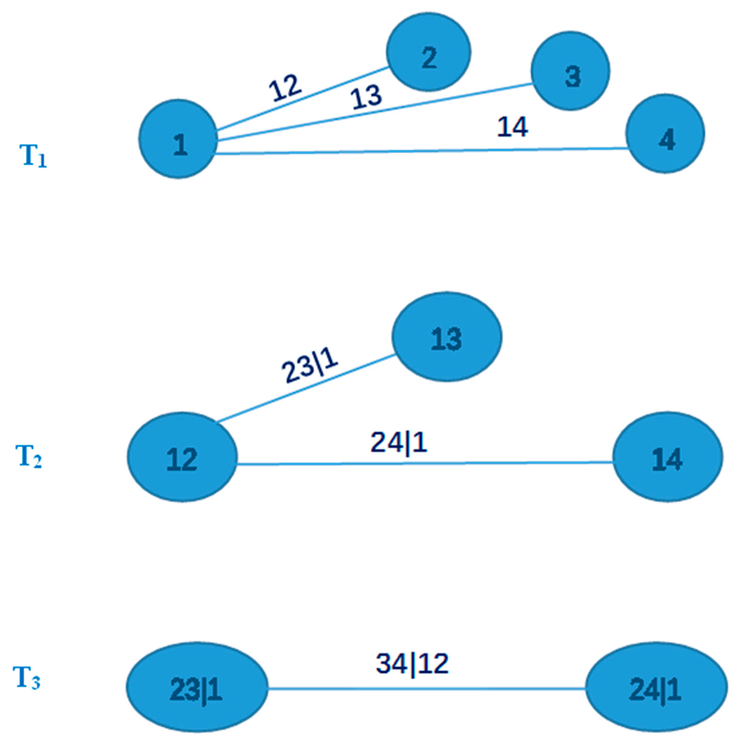
There are several pair-copula structures in higher-dimensional joint distributions. C-vine (canonical vine) and D-vine are two special types of vines. If key variables, that guide the other variables, can be found in the data, C-vine would be suitable for modeling. As for n-dimensional variables, the C-vine pair-copula structure consists of n − 1 trees; each tree Tj has one node connected to n − 1 edges. Figure 2 indicates the structure of a 4-dimensional C-vine [37].
It can be obtained from the C-vine structure that the general form of the C-vine density of a n-dimensional variable is:
f ( x 1 , x 2 , , x n ) = k = 1 n f ( x k ) j = 1 n 1 i = 1 n j c j , j + i | 1 , , j 1 ( F ( x j | x 1 , , x j 1 ) , F ( x j + i | x 1 , , x j 1 ) ) .
The maximum-likelihood estimation method is adopted to estimate the parameters of a C-vine pair-copula function [37].

2.2.3. Three-Dimensional C-Vine Pair-Copula Function Probability Calculation

There is no explicit function expressing the C-vine pair-copula probability distribution. Thus, this paper adopts numerical integration to calculate [38]. For a 3-dimensional variable ( X 1 , X 2 , X 3 ) , there is:
F ( x 1 , x 2 , x 3 ) = x 1 x 2 x 3 f ( x 1 , x 2 , x 3 ) d x 1 d x 2 d x 3 = x 1 x 2 x 3 f ( x 1 ) f ( x 2 ) f ( x 3 ) c 12 [ F 1 ( x 1 ) , F 2 ( x 2 ) ] c 23 [ F 2 ( x 2 ) , F 3 ( x 3 ) ] c 13 | 2 [ F ( x 1 | x 2 ) , F ( x 3 | x 2 ) ] d x 1 d x 2 d x 3 = x 1 x 2 x 3 c 12 [ F 1 ( x 1 ) , F 2 ( x 2 ) ] c 23 [ F 2 ( x 2 ) , F 3 ( x 3 ) ] c 13 | 2 [ F ( x 1 | x 2 ) , F ( x 3 | x 2 ) ] d F 1 ( x 1 ) d F 2 ( x 2 ) d F 3 ( x 3 ) = x 1 x 2 x 3 C 13 | 2 [ F ( x 1 | x 2 ) , F ( x 3 | x 2 ) ] F ( x 1 | x 2 ) F ( x 3 | x 2 ) F ( x 1 | x 2 ) F 1 ( x 1 ) F ( x 3 | x 2 ) F 2 ( x 2 ) d F 1 ( x 1 ) d F 2 ( x 2 ) d F 3 ( x 3 ) .
Assume x 1 , x 2 , x 3 are s , t , m , respectively, and their marginal distributions are u , v , w , respectively. Then, d F 1 ( x 1 ) = d u 1 , d F 2 ( x 2 ) = d u 2 , d F 3 ( x 3 ) = d u 3 . It can be obtained, through integral variable substitution, that:
F ( x 1 , x 2 , x 3 ) = s t m f ( x 1 , x 2 , x 3 ) d x 1 d x 2 d x 3 = 0 u 0 v 0 w 2 C 13 | 2 [ C 12 [ u 1 , u 2 ] u 2 , C 23 [ u 2 , u 3 ] u 2 ] u 1 u 3 d u 1 d u 2 d u 3 = 0 v C 13 | 2 [ C 12 [ u 1 , u 2 ] u 2 , C 23 [ u 2 , u 3 ] u 2 ] d u 2 .
This is the 1-dimensional integration of the copula distribution with 2-dimensional conditions. The 3-dimensional probability distribution can be solved through Gaussian Quadrature.

2.2.4. Calculation of the Synchronous and Asynchronous Probability of High–Low Runoff–Sediment

The dividing frequency of high–low runoff is set as p f = 75 % , p k = 25 % , and the corresponding dividing annual runoff of high–low runoff is recorded as X p f and X p k . When the runoff X satisfies X X p f , it is regarded as a high runoff; when the runoff X satisfies X p f X X p k , it is regarded as normal runoff; and when the runoff X satisfies X X p k , it is regarded as low runoff. The high–low assessment for sediment yield is defined similarly.
Assuming F(x1, x2, x3) to be the joint distribution function for the annual runoff of the 3 different stations, F(0.25, 0.25, 0.25) could be calculated by using formula (11); therefore, the value presents the probability when the annual runoff of the stations are all at their lowest. Consequently, the probabilities could also be available when they at their highest and at a normal level for the stations. Adding up the three probabilities, we derive the synchronous probability of annual runoff; then, the asynchronous probability is obtained as 1 minus the synchronous probability. Similarly, the synchronous and asynchronous probability of sediment could be calculated in the same way.

3. Results and Discussion

3.1. Division of the Study Intervals

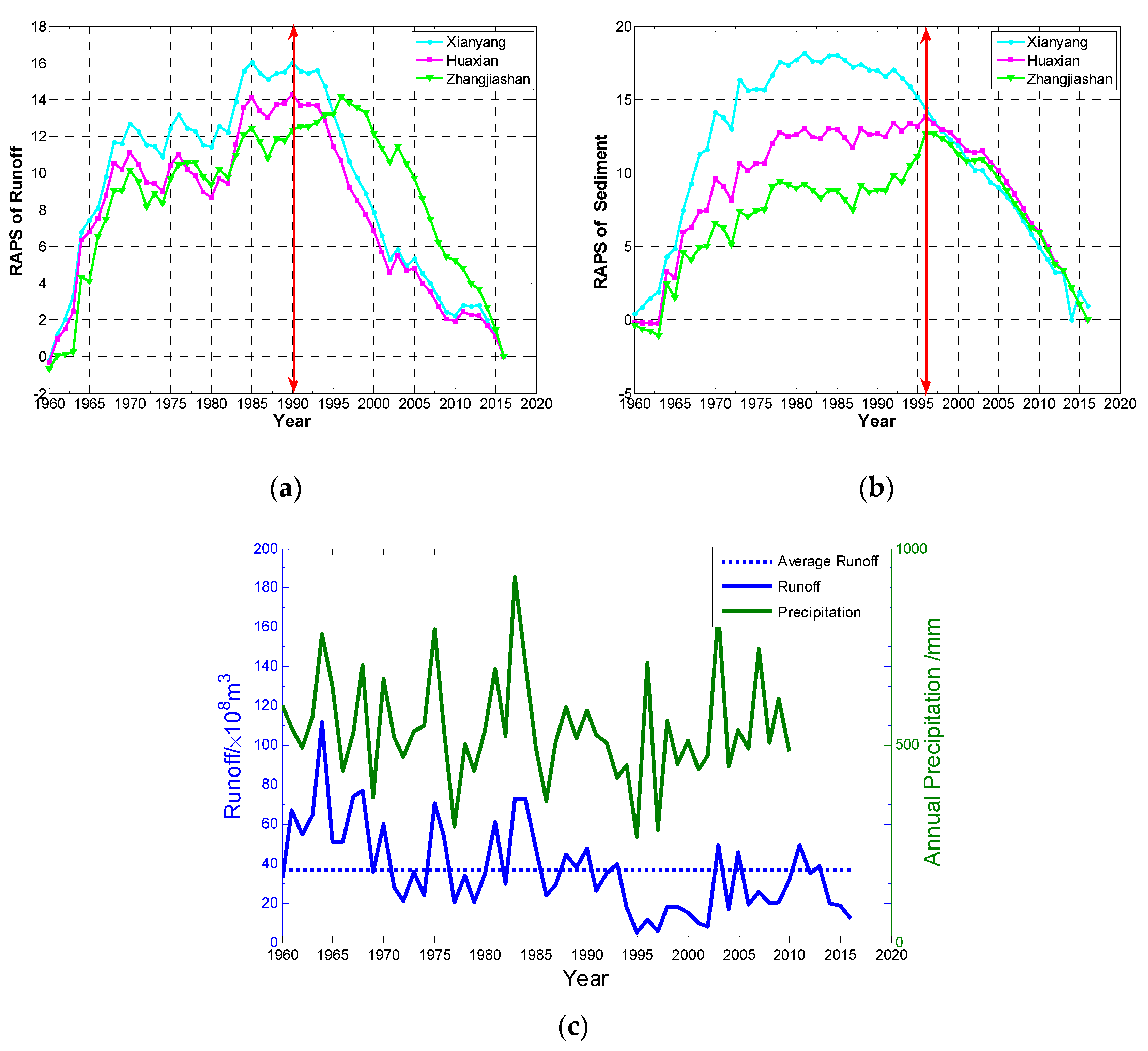
The RAPS values of the annual runoff and sediment yields of the Xianyang, Zhangjiashan, and Huaxian Stations, from 1960 to 2010, were calculated. Figure 3 shows the variation tendencies of the RAPS values.
It can be inferred from Figure 3 that the RAPS curves of runoff yield of the stations are consistent, among which the runoff consistency between Xianyang and Huaxian Stations is better. The RAPS curves also indicate that the sediment yield of Zhangjiashan and Huaxian Stations are consistent. Considering the locations and runoff–sediment data of these stations, it can be concluded that Zhangjiashan Station has a larger impact on Huaxian Station, in terms of sediment yield; while Xianyang Station has larger impact on Huaxian Station, in terms of runoff yield.
Furthermore, from Figure 3a, it can be seen that RAPS values, for both the Huaxian and Xianyang Stations, were maximal in the year 1990. Comparatively, the RAPS value was increasing before 1990, and decreasing from 1990 to 2016; it manifests that, before 1990, runoff was high for the two stations, while it decreased largely after 1990; furthermore, dramatic dropping-off occurred after 1993. On one hand, this related to climate changes such as rainfall, temperature, and so on; on the other hand, it was due to massive exploration of water resources within the Weihe River basin. For rainfall, annual runoff, and average runoff, please see Figure 3c. Stations upstream of the Xianyang Station had similar rainfall, which decreased slightly over a long period of time.
It can be inferred, from Figure 3b, that: The sediment RAPS values of the Huaxian and Zhangjiashan Stations reached their maximum in 1996, while that of Xianyang Station reached a maximum in 1981. This paper shall will take the inflection point of the Huaxian Station as the division point of data of the 3 stations. Hence, the time intervals for data analysis of sediment yields are divided into 1960–1996 and 1996–2016.
Why didn’t maximal sediment volume and maximal runoff volume occur in the same year? The reason is that annual sediment strongly correlates to annual runoff volume; however, sediment also is constrained by rainfall type, vegetation status, landforms, human activities, and so on, in the same year. Therefore, the maximal RAPS value of the runoff volume at the Huaxian Station is in 1990, and maximal RAPS value of sediment appears in 1996. To study the influences on Huaxian Station, exerted by runoff volume and sediment volume from other two stations, the year of maximal RAPS at Huaxian Station was selected to divide the time interval.

3.2. Establishment of the Marginal Distribution Function

Establishment of the 2D Joint Distribution Functions

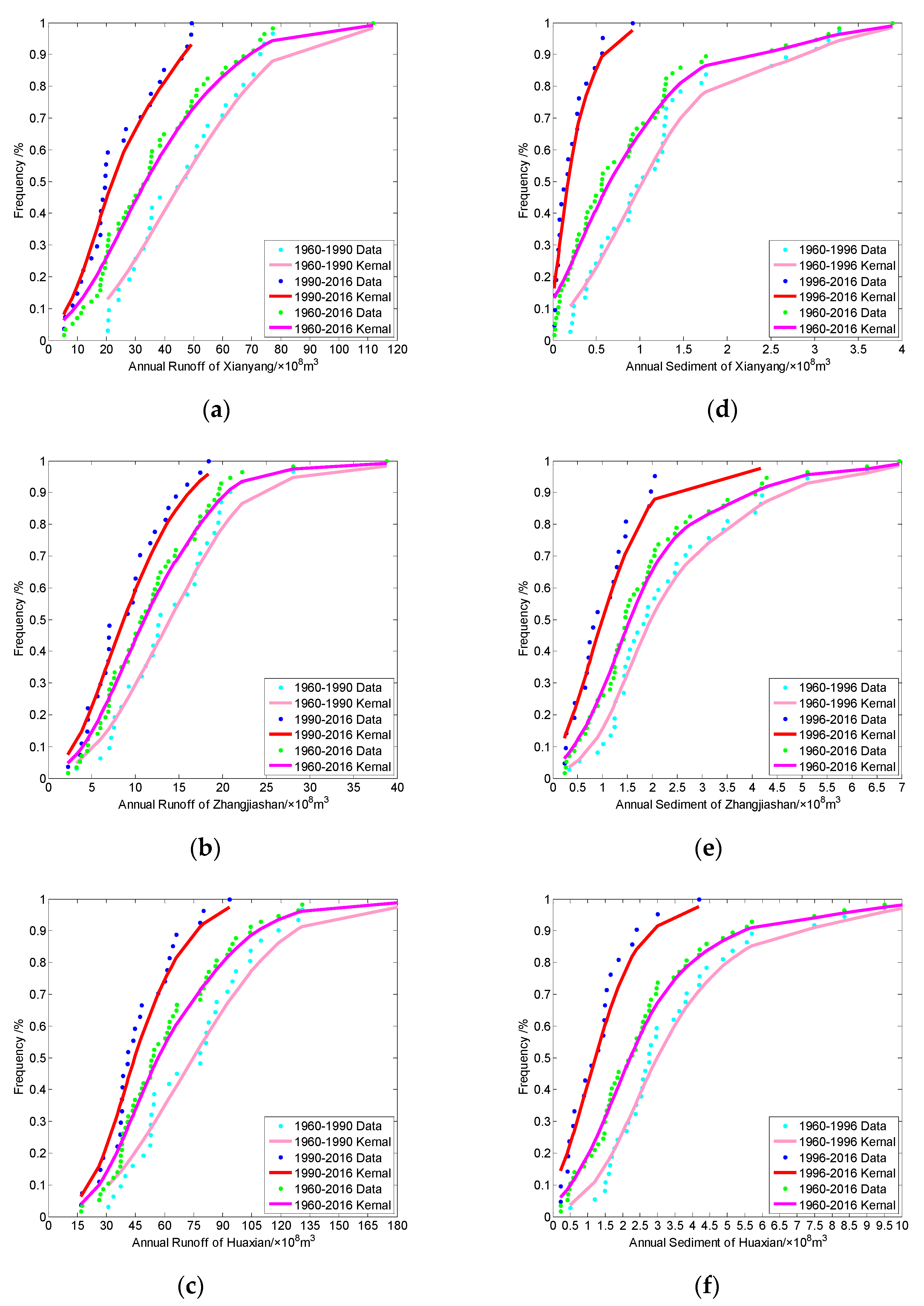
In order to establish the joint distribution functions of the runoff and sediment yields of the three stations, it is necessary to define the marginal distribution functions. According to kernel distribution theory, this paper adopts a Gaussian Kernel to separately fit the marginal distribution functions of the runoff and sediment yields in different time intervals and tests the distributions through the K–S Method (Kolmogorov–Smirnov goodness-of-fit test) [39,40,41], in which D represents the test statistics. The results of the K–S Test are listed in Table 1, while the function fitting results are shown in Figure 4.
It can be inferred, from Table 1, that if the significance level is 0.05, all the p-values fitted through the kernel distribution method will be greater than 0.05, and so they pass the test. Therefore, the kernel distribution can be adopted to fit the marginal distribution functions. Additionally, Figure 4 also shows, directly, that the kernel distribution function fits the marginal distribution functions of the runoff and sediment yields of the three stations well.

3.3. Analysis on the Runoff–Sediment Relationships between the Three Stations through Joint Distribution Functions

3.3.1. Analysis on Runoff–Sediment Probability of the Three Stations through Pair-Copula Function

The correlations of runoff yields, in different time intervals, of the three stations are demonstrated in Figure 5a–i. The correlations of sediment yields are demonstrated in Figure 5j–r.
From Figure 5a–i, we can infer that the correlation of runoff between the Xianyang and Huaxian Stations is the highest, especially during 1960–1990. The correlation of runoff between the Zhangjiashan and Huaxian Stations is relatively high. From Figure 5j–r, we can see that the correlation of sediment between the Zhangjiashan and Huaxian Stations is the highest; however, during 1996–2016, sediment yields of the Xianyang and Huaxian Stations are somehow related, but their correlation is relatively low.
Furthermore, this paper adopts R packages [42,43] to estimate the parameter θ of the copula function. In order to make the solution for the pair-copula function easier to obtain, this paper chose the optimal copula function among all the common functions frequently adopted in the fields of hydrology, including the Gumbel, Frank, and Clayton-copula functions. Additionally, this paper tests the copula function through Rosenblatt’s transformation method, proposed in [32], in which 5000 Monte Carlo simulations were used. See Table 2 for calculation results.
It can be inferred, from Table 2, that if the significance level is 0.05, then the C-vine pair-copula functions we built will pass the test, which could then be used to describe the joint distribution functions of annual runoff and annual sediment yields of the Xianyang, Zhangjiashan, and Huaxian Stations.

3.3.2. Probability Analysis on High–Low runoff and Sediment Yield of the Three Stations

The high–low runoff and sediment probability of the three stations can be calculated through the C-vine copula function in Table 2. The probabilities of synchronous and asynchronous high–low runoff–sediment of the three stations are listed in Table 3.
We can learn, from Table 3, that the probability of synchronous high–low runoff yields of the lower Weihe River’s Huaxian and Xianyang Stations, and the Jinghe River’s Zhangjiashan Station reached their maximum value in 1960–1990; which was approximately 73% and was obviously greater than the asynchronous probability. From 1990 to 2016, the synchronous probability descended sharply and was slightly less than that of the asynchronous probability. However, the synchronous probability of high–low sediment yields changed little, which was a bit higher than the asynchronous probability.
According to the research on the runoff–sediment utilization along the Jinghe and Weihe Rivers, we have found that, since the 1990s, as the social economy boosted, the development and utilization of the water resources of the Jinghe River increased significantly in river basins upstream of the Zhangjiashan Station, which, to some extent, impacted the probability of synchronous high–low runoff yields of the Huaxian, Zhangjiashan, and Xianyang Stations from 1990 to 2016.
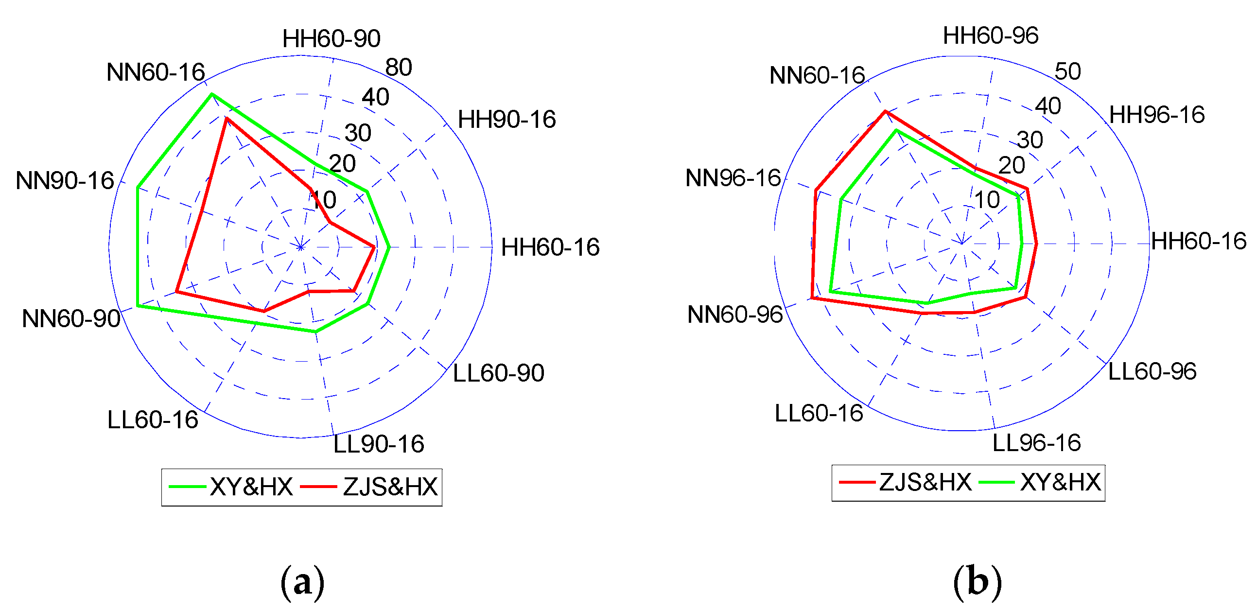
Additionally, synchronous probabilities of high–low runoff yields between every two stations in different time intervals were calculated by a C-vine pair-copula function, built through Table 2: The probability of synchronous high–low runoff–sediment yields of the Xianyang and Huaxian Stations, and the probability of synchronous high–low runoff–sediment yields of the Zhangjiashan and Huaxian Stations. The results are demonstrated in Figure 6.
It can be inferred, from Figure 6, that the probability of synchronous high–low runoff of the Huaxian and Xianyang Stations was obviously greater than that of the Huaxian and Zhangjiashan Stations; while the probability of synchronous high–low sediment of the Huaxian and Zhangjiashan Stations was obviously greater than that of the Huaxian and Xianyang Stations. The results indicate that the runoff yield of the lower Weihe River mostly came from Xianyang Station, in the middle reaches; meanwhile, the sediment yield of the lower Weihe River mostly came from Zhangjiashan Station, in the tributary Jinghe River. This is consistent with the conclusion drawn by Fuqiang Chen [44] and Xinwu Tu [45], using the ratio of water and sediment of the three hydrologic stations. Also, the probability of synchronous high–low runoff of the Weihe River’s Huaxian Station and the Jinghe River’s Zhangjiashan Station in 1960–1990 is obviously greater than that in 1990–2016, while the probability of synchronous high–low runoff of the Huaxian and Xianyang Stations changes little between 1960–1990 and 1990–2016. In accordance with Figure 3, the major reason for this phenomenon is that the annual runoff, from 1990 to 1996, for the Zhangjiashan Station, was in high runoff period; in contrast, the runoff at Huaxian Station was in low runoff in the same period. That is, the high and low runoff of the two stations are obviously not in the same period. Moreover, the Zhangjiashan Station is situated the upstream of the Huaxian Station, and a high annual runoff at Zhangjiashan doesn’t bring a high annual runoff to Huaxian, downstream. Therefore, the characteristic of water coming to Huaxian from Zhangjiashan isn’t obvious. However, the synchronous probability of the high and low runoff at Xianyang and Huaxian was always larger than 90% in 1960–1990 and 1990–2016, which shows the characteristic of water coming to Huaxian from Xianyang more obviously.
Next, this paper adopts the C-vine pair-copula function and conditional probability formulas, built through Table 2, to calculate the probabilities of high runoff (sediment) of the Huaxian Station caused, respectively, by high, normal, and low runoff (sediment) of the Xianyang Station, and the probabilities of high runoff (sediment) of the Huaxian Station caused, respectively, by high, normal, and low runoff (sediment) of the Zhangjiashan Station, which are listed in Table 4. Probabilities of low runoff (sediment) of the Huaxian Station caused, respectively, by high, normal, and low runoff (sediment) of the Xianyang Station and the probabilities of low runoff (sediment) of the Huaxian Station caused, respectively, by high, normal, and low runoff (sediment) of the Zhangjiashan Station are demonstrated in Table 5.
In Table 4, from 1990 to 2016, the probability was 91% for the high runoff at Huaxian Station being caused by high runoff at Xianyang Station; while the probability is no less than 9% for the high runoff at Huaxian Station being caused by normal runoff at Xianyang Station; which means the high runoff at Huaxian Station is very unlikely to have resulted from low runoff at Xianyang Station. The probability shows 47% for the high runoff at Huaxian being caused by the high runoff at Zhangjiashan—the probability was decreased by 44%, compared with the one at Xianyang. The probability of the high runoff at Huaxian being caused by normal runoff at Zhangjianshan is 41%, and it was 12% likely to have resulted from low runoff at Zhangjiashan. The data depict that, from 1990 to 2016, the high runoff at Huaxian was mainly because of high runoff at Xianyang. Besides, from Table 4, from 1960 to 1990, the high runoff at Huaxian was mainly because of the high runoff at Xianyang, no matter whether it was in 1960–1996 or in 1996–2016, the high sediment at Huaxian Station was mainly caused by Zhangjiashan Station. It may also be the same case, that a low runoff at Huaxian Station was caused by Xianyang Station, from Table 5; however, the low sediment at Huaxian Station was influenced by Zhangjiashan Station.

3.3.3. Probability Control of Runoff and Sediment Yield of the Three Stations

As the social economy boosts, the utilization range and amount of runoff–sediment resources of the Weihe River also vary. The burning problem is to control and guarantee the reasonable allocation of the runoff–sediment resource utilization of the upstream and downstream Weihe River, effectively. Hence, this paper adopted joint distribution functions and conditional probability formulas to calculate the conditional probabilities we need, and to guarantee the balance between runoff yield and sediment yield of both the upstream and downstream Weihe River and its tributary, the Jinghe River, at a relatively large probability. Utilizing the formula of conditional probability, the marginal distribution function and C-vine pair-copula function, built using the 1990–2016 runoff yields and considering the regulation abilities upstream of the Huaxian Station in high runoff years, the adjusted frequency will be set as 0.4 < prunoff < 0.6. Then, if the runoff frequencies of the Xianyang and Zhangjiashan Stations, which are located upstream of the Huaxian Station, are set as 0.4 < prunoff < 0.6, then the probability that the runoff frequency of the Huaxian Station is 0.4 < prunoff < 0.6 (40.82 × 10⁸ m3 < Xrunoff < 48.1 × 10⁸ m3) will be 0.778. Similarly, in low runoff years, considering the regulation abilities upstream of the Huaxian Station, the runoff frequency is 0.1 < prunoff < 0.25, and the calculation results are listed in Table 6. If further soil and water conservation works are strengthened upstream of the Huaxian Station, as well as decontamination of the river channels on a regular basis, the sediment yield of the downstream Weihe River will reduce significantly. Considering the present measures upstream of the Huaxian Station, and applying the marginal distribution function and C-vine copula function built using the 1996–2016 sediment yields, the adjusted frequencies of sediment yields of the three stations are measured and calculated, respectively, with 0.4 < psediment < 0.6 in high sediment years, and 0.1 < psediment < 0.25 in low sediment years. See Table 6 for the calculation results.
The following can be inferred from Table 6: In low runoff years, if the annual runoff yield of the Xianyang Station is adjusted to somewhere between 5.80 × 10⁸ m3 and 14.50 × 10⁸ m3, while that of the Zhangjiashan Station is between 2.30 × 10⁸ m3 and 5.60 × 10⁸ m3, then the probability of the annual runoff yield of the Huaxian Station being between 17.80 × 10⁸ m3 and 32.50 × 10⁸ m3 will be 70.55%. Similarly, in high runoff years, if the annual runoff yield of the Xianyang Station is adjusted to somewhere between 18.70 × 10⁸ m3 and 26.50 × 10⁸ m3, while that of the Zhangjiashan Station is between 7.00 × 10⁸ m3 and 10.10 × 10⁸ m3, then the probability of annual runoff yield of the Huaxian Station being between 40.82 × 10⁸ m3 and 48.10 × 10⁸ m3 will be 77.8%. If the annual sediment yield of the Xianyang Station is adjusted to somewhere between 0.22 × 10⁸ m3 and 1.21 × 10⁸ m3, then the probability of annual sediment yield of the Huaxian Station being between 0.92 × 10⁸ m3 and 1.49 × 10⁸ m3 is 81.56%. In practical applications, different conditional probabilities can also be calculated, as needed, through the established joint distribution functions and conditional probability formulas.

4. Conclusions

The characteristics of high–low runoff–sediment variation are closely related to river regime stability, channel evolution, and river–lake relations, among other aspects. Studying the characteristics of high–low runoff–sediment yields of rivers is essential in revealing the sediment-evolutionary relationships of rivers and administrating runoff–sediment resources. Compensation relationships of runoff and sediment can be found between the upstream and downstream, and the mainstream and branches of rivers. Analyzing the encounter frequency of high–low runoff and sediment yield is important for the appropriate dispatching of runoff–sediment resources, as well as river regulation. This paper emphasizes the certain probability relationships of runoff yield and sediment yield between different hydrologic stations in different reaches of the river and introduces the pair-copula function for analyzing the high–low runoff–sediment compensation characteristics. The data adopted in this paper come from the observation data of three stations of the Weihe River and its tributary, the Jinghe River. The conclusions are as follows:
(1)
The pair-copula function is flexible in adoption and simple in parameter solution. It has obvious advantages, in terms of building multidimensional joint distribution functions. Kernel distribution theory and C-vine pair-copula functions were used to obtain the annual runoff and sediment marginal distribution functions and the runoff–sediment joint distribution functions of the three stations of the Weihe River, in different time intervals, accurately.
(2)
The synchronous and asynchronous encounter probabilities of high–low runoff between the three stations, and between each pair of stations, were accurately calculated. Meanwhile, through conditional probability formulas, the probabilities that the high, normal, and low status of runoff and sediment yield of downstream hydrologic stations were caused by different statuses of different upstream stations were also calculated.
(3)
The designed runoff–sediment yields of upstream stations were estimated, in order to guarantee the runoff–sediment yields of downstream stations being in a certain range, in high and low runoff years, respectively.
The C-vine pair-copula function was built, according to the annual data of runoff and sediment yields of the three stations and the encounter frequencies of synchronous high–low runoff–sediment, as well as different conditional probabilities, were obtained. Furthermore, if the joint distribution function can be built on the basis of monthly data, according to which the encounter frequency of synchronous high–low runoff–sediment in flood and non-flood seasons can be obtained, the study will then be in better practice.

Author Contributions

This study was designed and the analysis method was provided by Q.Y. The data were prepared by Y.L. and Q.Y. The manuscript was prepared by Q.Y. and revised by H.J., Y.L., Z.L. and Z.G. The manuscript was checked by Q.Y., H.J., Y.L., Z.L. and Z.G.

Funding

This research is funded by the ‘111’ Discipline Innovation and Intelligence Base Project of Hydro-Eco and Water Security in Arid and Semi-Arid Regions, proposed by the Ministry of Education and State Administration of Foreign Experts Affairs P. R. China (Grant No. B08039); the Natural Science Basic Research Plan in Shaanxi Province of China (2018JM1045); the Xi’an Construction Science and Technology Planning Project (SJW2017–11); the National Natural Science Foundation of China (41471452); the Special Fund for Basic Scientific Research Operating Expenses of Central Universities (natural science) (310829161010, the Effects of Water-Saving Irrigation Patterns on Groundwater in Northwest Area); and the Special Fund for Basic Scientific Research of Central Colleges (Program No. 300102299206).

Conflicts of Interest

The authors declare no conflict of interest.

References

  1. Guo, S.L.; Yan, B.W.; Xiao, Y.; Fang, B.; Zhang, N. Multivariate Hydrological Analysis and Estimation. J. China Hydrol. 2008, 28, 1–7. [Google Scholar]
  2. Correia, F.N. Multivariate partial duration series in flood risk analysis. In Hydrologic Frequency Modeling; Springer: Dordrecht, The Netherlands, 1987; pp. 541–554. [Google Scholar]
  3. Kotz, S.; Balakrishnan, N.; Johnson, N.L. Continuous Multivariate Distributions; Wiley: New York, NY, USA, 2000; pp. 31–60. [Google Scholar]
  4. Lall, U.; Bosworth, K. Multivariate kernel estimation of functions of space and time. In Stochastic and Statistical Methods in Hydrology and Environmental Engineering; Springer: Dordrecht, The Netherlands, 1994; pp. 56–89. [Google Scholar]
  5. De Michele, C.; Salvadori, G. A generalized Pareto intensity-duration model of storm rainfall exploiting 2-Copulas. J. Geophy. Res. Atmos. 2003, 108, 4067. [Google Scholar] [CrossRef]
  6. De Michele, C.; Salvadori, G.; Canossi, M.; Petaccia, A.; Rosso, R. Bivariate Statistical Approach to Check Adequacy of Dam Spillway. J. Hydrol. Eng. 2005, 10, 50–57. [Google Scholar] [CrossRef]
  7. Salvadori, G.; De Michele, C. Statistical characterization of temporal structure of storms. Adv. Water Resour. 2006, 29, 827–842. [Google Scholar] [CrossRef]
  8. Salvadori, G.; De Michele, C.; De Michele, C. Multivariate return period calculation via survival functions. Water Resour. Res. 2013, 49, 2308–2311. [Google Scholar] [CrossRef] [Green Version]
  9. Fan, L.; Wang, H.; Liu, Z.; Li, N. Quantifying the relationship between drought and water scarcity using Copulas: Case study of Beijing–Tianjin–Hebei metropolitan areas in China. Water 2018, 10, 1622. [Google Scholar] [CrossRef]
  10. Razmkhah, H.; AkhoundAli, A.M.; Radmanesh, F.; Saghafian, B. Evaluation of rainfall spatial correlation effect on rainfall-runoff modeling uncertainty, considering 2-copula. Arab. J. Geosci. 2016, 9, 125–138. [Google Scholar] [CrossRef]
  11. Liu, Y.; Liu, Y.; Hao, Y.; Wang, T.; Yeh, T.C.; Fan, Y.; Zhang, Q. Probabilistic analysis of extreme discharges and precipitations with a nonparametric Copula Model. Water 2018, 10, 823. [Google Scholar] [CrossRef]
  12. Liu, C.L.; Zhou, Y.W.; Sui, J.; Gao, L. Research of methodology of multivariate analysis of design storm based on 3-copula function. J. Harbin Inst. Technol. 2015, 47, 87–92. [Google Scholar]
  13. Pham, M.T.; Vernieuwe, H.; De Baets, B.; Willems, P.; Verhoest, N.E.C. Stochastic simulation of precipitation-consistent daily reference evapotranspiration using vine copulas. Stoch. Environ. Res. Risk Assess. 2016, 30, 2197–2214. [Google Scholar] [CrossRef]
  14. Gyasi-Agyei, Y.; Melching, C.S. Modelling the dependence and internal structure of storm events for continuous rainfall simulation. J. Hydrol. 2012, 464, 249–261. [Google Scholar] [CrossRef]
  15. Ridolfi, E.; Montesarchio, V.; Rianna, M.; Sebastianelli, S.; Russo, F.; Napolitano, F. Evaluation of Rainfall Thresholds Entropy: Influence of Bivariate Distribution Selection. Irrig. Drain. 2013, 62, 50–60. [Google Scholar] [CrossRef]
  16. Gräler, B.; van den Berg, M.; Vandenberghe, S.; Petroselli, A.; Grimaldi, S.; De Baets, B.; Verhoest, N. Multivariate return periods in hydrology: A critical and practical review focusing on synthetic design hydrograph estimation. Hydrol. Earth Syst. Sci. 2013, 17, 1281–1296. [Google Scholar] [CrossRef]
  17. Wahl, T.; Mudersbach, C.; Jensen, J. Assessing the hydrodynamic boundary conditions for risk analyses in coastal areas: A multivariate statistical approach based on Copula functions. Nat. Hazards Earth Syst. Sci. 2012, 12, 495–510. [Google Scholar] [CrossRef]
  18. Chen, L.; Singh, V.P.; Guo, S.L.; Hao, Z.C.; Li, T.Y. Flood Coincidence Risk Analysis Using Multivariate Copula Functions. J. Hydrol. Eng. 2012, 17, 742–755. [Google Scholar] [CrossRef]
  19. Guo, A.J.; Chang, J.X.; Wang, Y.M.; Huang, Q. Variations in the Runoff–sediment Relationship of the Weihe River Basin Based on the Copula Function. Water 2016, 8, 223. [Google Scholar] [CrossRef]
  20. Wang, M.L.; Xia, C.Y.; Lu, C.S.; Huang, J. Analysis of variation trend of water and sediment in jinsha river basin. Yangtze River 2008, 39, 15–22. [Google Scholar]
  21. Wang, P.; Fang, G.; Guo, Y.; Wen, X. Reseach on water resources optimal scheduling based on improved Quantum Genetic algorithm. J. China Three Gorges Univ. (Nat. Sci.) 2016, 38, 7–13. [Google Scholar]
  22. Fu, Y. Inflow Analysis and Optimal Dispatching of Jinpen Reservoir in Shaanxi Province; Xi’an University of Technology: Xi’an, China, 2004; pp. 36–41. [Google Scholar]
  23. Huang, C.; Wang, Z.; Li, S.; Chen, S. A multi-reservoir operation optimization model and application in the upper Yangtze River Basin I. Principle and solution of the model. J. Hydrol. Eng. 2014, 45, 1009–1019. [Google Scholar]
  24. Guan, S.; Lin, Y.; Zha, X.; Ding, B.; Tao, N.; Liu, Z. Copula Function-Based Flood Coincidence Probability Analysis for Mainstream and Tributary of the Hanjiang River Basin. Acta Sci. Nat. Univ. Sunyatseni 2015, 54, 130–137. [Google Scholar]
  25. Huaxiong, L.; Yu, K.; Gottschalk, L. Estimation of the distribution of annual runoff from climatic variables using copulas. Water Resour. Res. 2014, 50, 7134–7152. [Google Scholar] [Green Version]
  26. Vernieuwe, H.; Vandenberghe, S.; De Baets, B.; Verhoest, N.E.C. A continuous rainfall model based on vine copulas. Hydrol. Earth Syst. Sci. 2015, 19, 2685–2699. [Google Scholar] [CrossRef] [Green Version]
  27. Poduje, A.C.C.; Haberlandt, U. Spatio-Temporal Synthesis of Continuous Precipitation Series Using Vine Copulas. Water 2018, 10, 862. [Google Scholar] [CrossRef]
  28. Shafaei, M.; Fakheri-Fard, A.; Dinpashoh, Y.; Mirabbasi, R.; De Michele, C. Modeling flood event characteristics using D-vine structures. Theor. Appl. Climatol. 2017, 130, 713–724. [Google Scholar] [CrossRef]
  29. Huang, S.; Liu, D.; Huang, Q.; Chen, Y. Contributions of climate variability and human activities to the variation of runoff in the Wei River Basin, China. Hydrol. Sci. J. 2016, 61, 1026–1039. [Google Scholar] [CrossRef]
  30. Zhu, H.Y.; Han, C.B.; Jia, Z.F.; Liu, Y.; Li, P.C. Analysis on characteristics of runoff and sediment of Zhangjiashan hydrological station and case study for Jing he River. Trans. CSAE 2012, 28, 48–55. [Google Scholar]
  31. Gao, P.; Geissen, V.; Ritsema, C.J.; Mu, X.M.; Wang, F. Impact of climate change and anthropogenic activities on stream flow and sediment discharge in the Wei River basin, China. Hydrol. Earth Syst. Sci. 2013, 17, 961–972. [Google Scholar] [CrossRef] [Green Version]
  32. Zhang, J.P.; Ding, Z.H.; Guo, B.T. Study on evolution trends and encounter risk of runoff and sediment in Jinghe river. Hydrol. Eng. 2015, 34, 11–16. (In Chinese) [Google Scholar]
  33. Chang, J.X.; Wang, Y.M.; Istanbulluoglu, E.; Bai, T.; Huang, Q.; Yang, D.W.; Huang, S.Z. Impact of climate change and human activities on runoff in the Weihe River Basin, China. Quat. Int. 2015, 380, 169–179. [Google Scholar] [CrossRef]
  34. Tadic, L.; Bonacci, O.; Dadic, T. Analysis of the Drava and Danube rivers floods in Osijek (Croatia) and possibility of their coincidence. Environ. Earth Sci. 2016, 9, 1238. [Google Scholar] [CrossRef]
  35. Sklar, A. Fonction de répartition à n dimensions et leurs marges. Publ. Inst. Stat. Univ. Paris 1959, 8, 229–231. [Google Scholar]
  36. Joe, H. Families of m-variate distributions with given margins and m(m−1)/2 bivariate dependence parameters. Distributions with Fixed Marginals and Related Topics. Lect. Notes-Monogr. Ser. 1996, 28, 120–141. [Google Scholar]
  37. Aas, K.; Czado, C.; Frigessi, A.; Bakken, H. Pair-copula constructions of multiple dependence. Insur. Math. Econ. 2009, 44, 182–198. [Google Scholar] [CrossRef] [Green Version]
  38. Rosenblatt, M. Remarks on a Multivariate Transformation. Ann. Math. Stat. 1952, 23, 470–472. [Google Scholar] [CrossRef]
  39. Genest, C.; Rémillard, B.; Beaudoin, D. Goodness-of-fit tests for copulas: A review and a power study. Insur. Math. Econ. 2009, 44, 199–213. [Google Scholar] [CrossRef]
  40. Zeng, Z. Application of Pair-Copulas Function in Drought Characteristics Analysis; Northwest A&F University: Yangling, China, 2012; pp. 24–27. [Google Scholar]
  41. You, Q.Y.; Liu, Y.; Liu, Z. Probability analysis of the water table and driving factors using a multidimensional Copula Function. Water 2018, 10, 472. [Google Scholar] [CrossRef]
  42. R Copula Package: Program R. R Version 3.5.0. Available online: https://cran.r-project.org/package=copula (accessed on 23 April 2018).
  43. R CDVine Package: Program R. R Version 3.5.0. Available online: https://cran.r-project.org/package=CDVine (accessed on 29 October 2015).
  44. Chen, F. Analysis of water-sand evolution characteristics in the lower reaches of weihe river. Shaanxi Water Resour. 2010, 1, 29–32. [Google Scholar]
  45. Tu, X. The Wei River Hydrology; Shaanxi Science and Technology Press: Xi’an, China, 2012; ISBN 9787536956865. [Google Scholar]
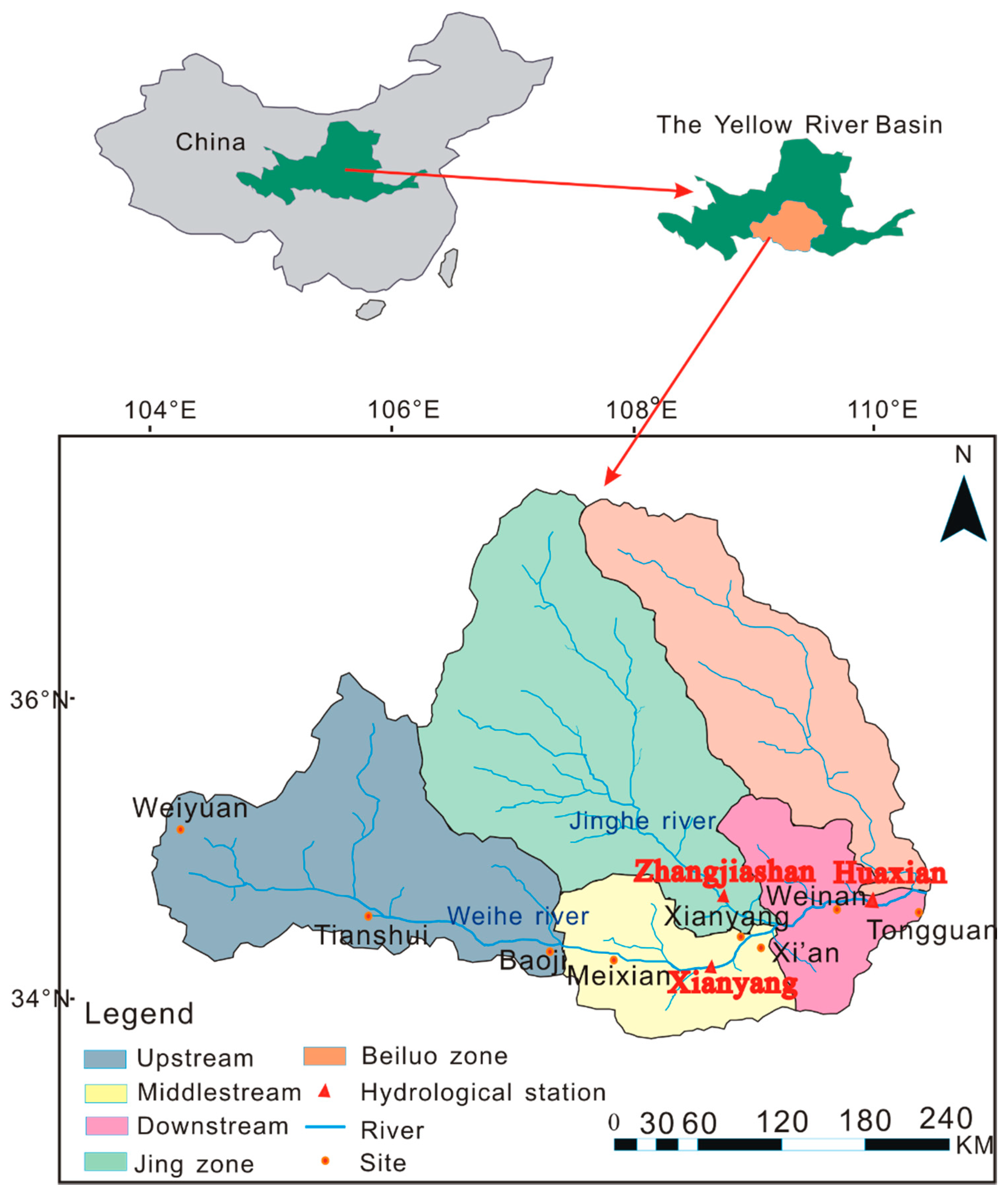
Figure 1. Locational map of the researching area.
Water 11 00510 g001
Figure 2. Structure of a 4-dimensional C-vine.
Water 11 00510 g002
Figure 3. Figure of annual runoff, sediment, and precipitation yield of Xianyang Station, Zhangjiashan Station, and Huaxian Station. (a) RAPS figure of annual runoff. (b) RAPS figure of annual sediment. (c) Figure of annual precipitation and runoff of Xianyang Station.
Water 11 00510 g003
Figure 4. The marginal distribution function diagram of annual runoff and sediment yield of the Three Stations: (a) Runoff of Xianyang Station. (b) Runoff of Zhangjiashan Station. (c) Runoff of Huaxian Station. (d) Sediment of Xianyang Station. (e) Sediment of Zhangjiashan Station. (f) Sediment of Huaxian Station.
Water 11 00510 g004
Figure 5. Correlation of runoff (ai) and sediment (jr) yields of the Three Stations.
Water 11 00510 g005aWater 11 00510 g005b
Figure 6. Probability of synchronous high–low runoff–sediment of the two stations. Note: HH stands for synchronous high runoff/sediment of the two stations; NN stands for normal runoff/sediment of the two stations; LL stands for synchronous low runoff/sediment of the two stations; and 60–90 stands for the time interval of 1960 to 1990, and similarly for the others. (a) is the probability of synchronous high–low runoff of the two stations, with unit of %; and (b) is the probability of synchronous high–low sediment of the two stations, with unit of %.
Water 11 00510 g006
Table 1. Function fitting results of marginal distribution.
RunoffYear1960–19901990–20161960–2016
Dp-ValueDp-ValueDp-Value
Xianyang0.09720.29030.12660.06100.06520.5564
Zhangjiashan0.08880.46950.10620.23480.05070.9680
Huaxian0.09330.36360.10180.31570.06630.5824
SedimentYear1960–19961996–20161960–2016
Dp-ValueDp-ValueDp-Value
Xianyang0.09820.18180.11710.31570.11560.0718
Zhangjiashan0.06810.91610.09950.67230.06460.6923
Huaxian0.09860.18580.10620.47150.06420.6703
Table 2. Selection and test of joint distribution functions of the runoff and sediment yields of the three stations.
C-VineYearVariablesCopulaθp-Value
Runoff1960–19903, 2Frank11.830.42
3, 1Frank36.22
1, 2; 3Frank−0.69
1990–2016 3, 2Gumbel1.350.53
3, 1Frank29.21
1, 2; 3Frank−0.91
1960–20163, 2Gumbel2.390.31
3, 1Gumbel8.14
1, 2; 3Frank−0.03
Sediment1960–19963, 1Gumbel2.500.07
3, 2Gumbel4.59
2, 1; 3Frank−7.73
1996–20163, 1Clayton2.820.40
3, 2Clayton7.18
2, 1; 3Frank−4.96
1960–20163, 1Frank10.270.31
3, 2Frank16.35
1, 2; 3Frank−4.44
Note: 1 represents the Value of Xianyang Station, 2 represents the value of Zhangjiashan Station, and 3 represents the value of Huaxian Station.
Table 3. Probabilities of synchronous and asynchronous high–low runoff–sediment of the three stations.
YearLLLNNNHHHSynchronousAsynchronous
Runoff1960–19900.18150.36260.18150.72560.2744
1990–20160.08860.24770.10820.44450.5555
1960–20160.14270.31460.17200.62930.3707
Sediment1960–19960.11540.28330.15410.55280.4472
1996–20160.17780.27230.08790.53200.4680
1960–20160.14850.30750.15960.61560.3844
Note: LLL stands for synchronous low runoff/sediment of the three stations; NNN stands for synchronous normal runoff/sediment of the three stations; and HHH stands for synchronous high runoff/sediment of the three stations.
Table 4. Probabilities of high runoff (sediment) of the Huaxian Station caused, respectively, by high, normal, and low runoff (sediment) of the Xianyang and Zhangjiashan Stations.
YearP(Hxy|Hhx)P(Hzjs|Hhx)P(Nxy|Hhx)P(Nzjs|Hhx)P(Lxy|Hhx)P(Lzjs|Hhx)
Runoff1960–19900.92360.77440.07640.224800.0008
1990–20160.90520.47320.09480.412800.1140
1960–20160.92440.72320.07560.263600.0132
Sediment1960–19960.73640.86240.25280.13720.01080.0004
1996–20160.56480.74880.42640.25120.00880
1960–20160.74520.87840.25280.12160.00200
Note: P is the probability; Hxy represents the high annual runoff/sediment yield of Xianyang Station; Hhx represents the high annual runoff/sediment yield of Huaxian Station; Nzjs represents the normal annual runoff/sediment yield of Zhangjiashan Station; and Lzjs represents the low annual runoff/sediment yield of Zhangjiashan Station; similarly for the others.
Table 5. Probabilities of low runoff (sediment) of the Huaxian Station caused, respectively, by high, normal, and low runoff (sediment) of Xianyang and Zhangjiashan Stations.
YearP(Hxy|Lhx)P(Hzjs|Lhx)P(Nxy|Lhx)P(Nzjs|Lhx)P(Lxy|Lhx)P(Lzjs|Lhx)
Runoff1960–199000.00080.07640.22480.92360.7744
1990–201600.11400.09480.49160.90520.3944
1960–201600.01320.11600.35960.88400.6272
Sediment1960–19960.01080.00040.34720.20200.6420.7976
1996–20160.008800.20640.09200.78480.9080
1960–20160.002000.24160.18080.75640.8192
Note: The meanings of P, Hxy, Lhx, Hzjs, Nxy, Nzjs, Lxy, Lhx, and Lzjs are the same as in Table 4.
Table 6. Typical conditional probability.
Typical Conditional Probability
RunoffP(40.82 < Runoffhx < 48.10|26.50 > Runoffxy > 18.70, 10.10 > Runoffzjs > 7.00) = 0.7780
P(32.50 < Runoffhx < 17.80|14.50 > Runoffxy > 5.80, 5.60 > Runoffzjs > 2.30) = 0.7055
SedimentP(1.49 > Sedihx > 0.92|0.22 > Sedixy > 0.12, 1.21 > Sedizjs > 0.80) = 0.8156
P(0.57 > Sedihx > 0.41|0.074 > Sedixy > 0.06, 0.61 > Sedizjs > 0.22) = 0.9517
Note: Runoffhx represents the annual runoff yield of the Huaxian Station, Runoffxy represents the annual runoff yield of the Xianyang Station, Runoffzjs represents the annual runoff yield of the Zhangjiashan Station; all the units are 108 m3. Sedihx represents the annual sediment yield of the Huaxian Station, Sedixy represents the annual sediment yield of the Xianyang Station, Sedizjs represents the annual sediment yield of the Zhangjiashan Station; all the units are 108 m3.