Evaluation of Drydown Processes in Global Land Surface and Hydrological Models Using Flux Tower Evapotranspiration


Abstract
:1. Introduction
2. Materials and Methods
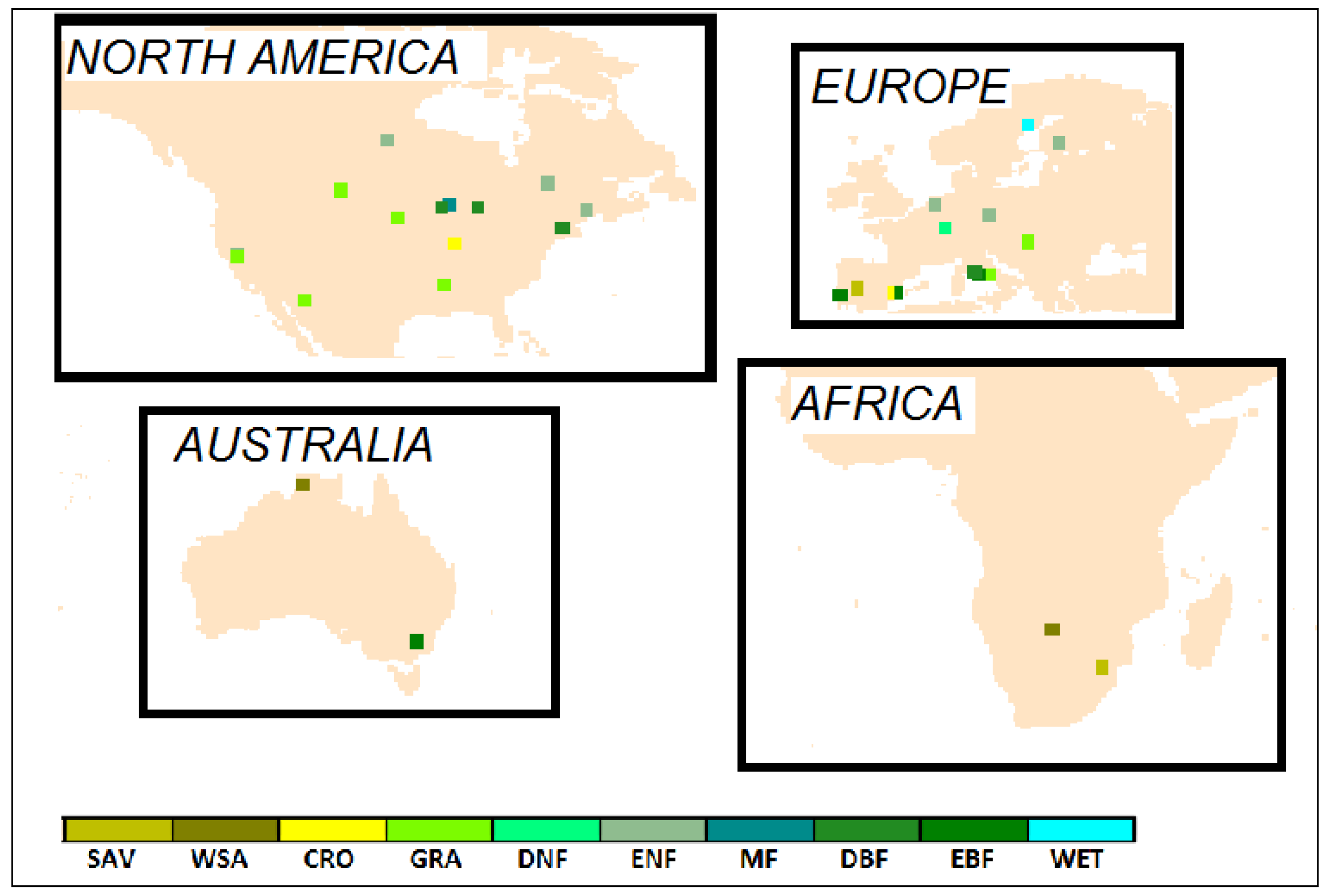
2.1. Flux Tower Data
2.2. Model Data
2.3. Defining the Metric
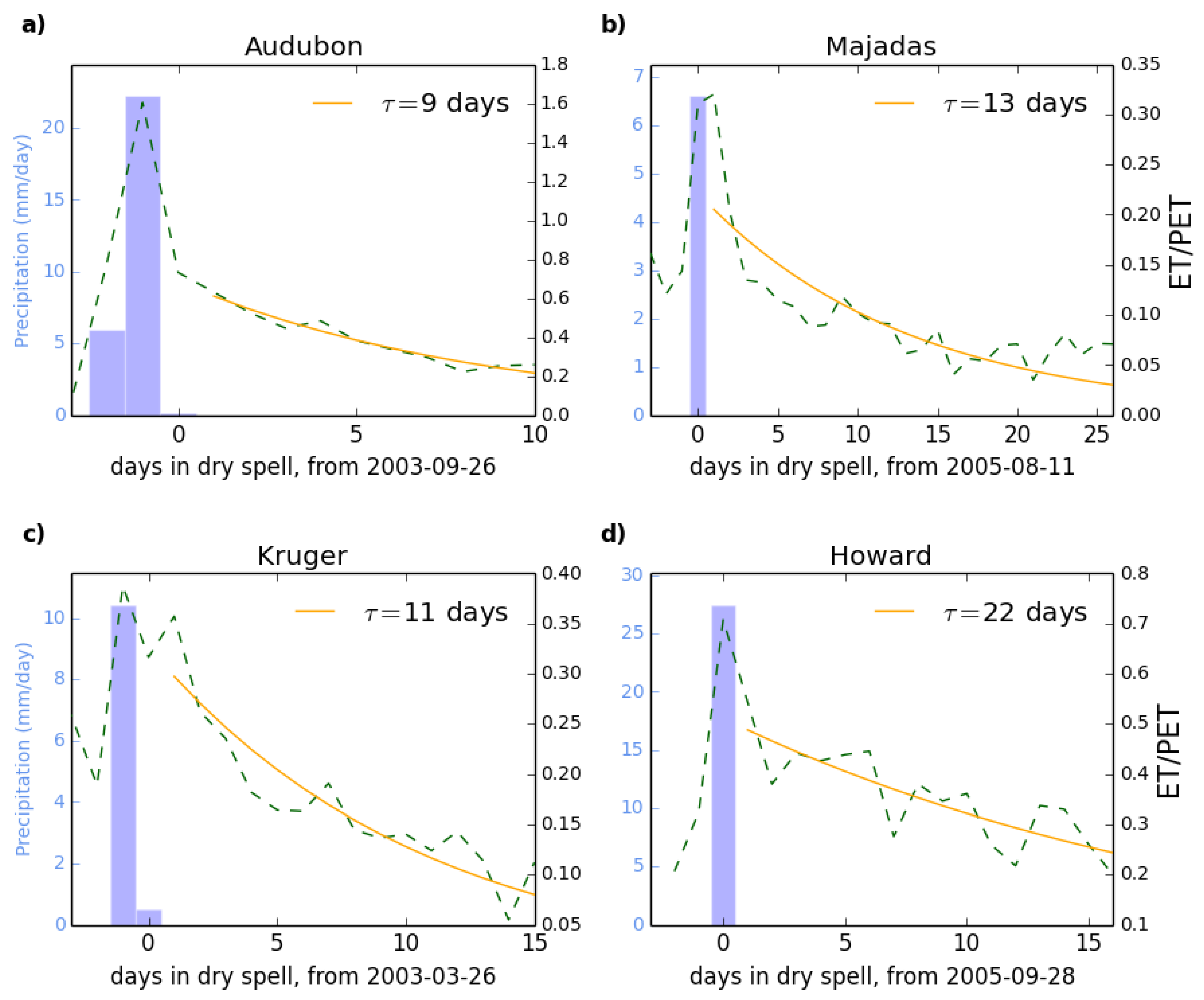
2.4. Applying the Metric to the Flux Tower Data
2.5. Applying the Metric to the Models
3. Results
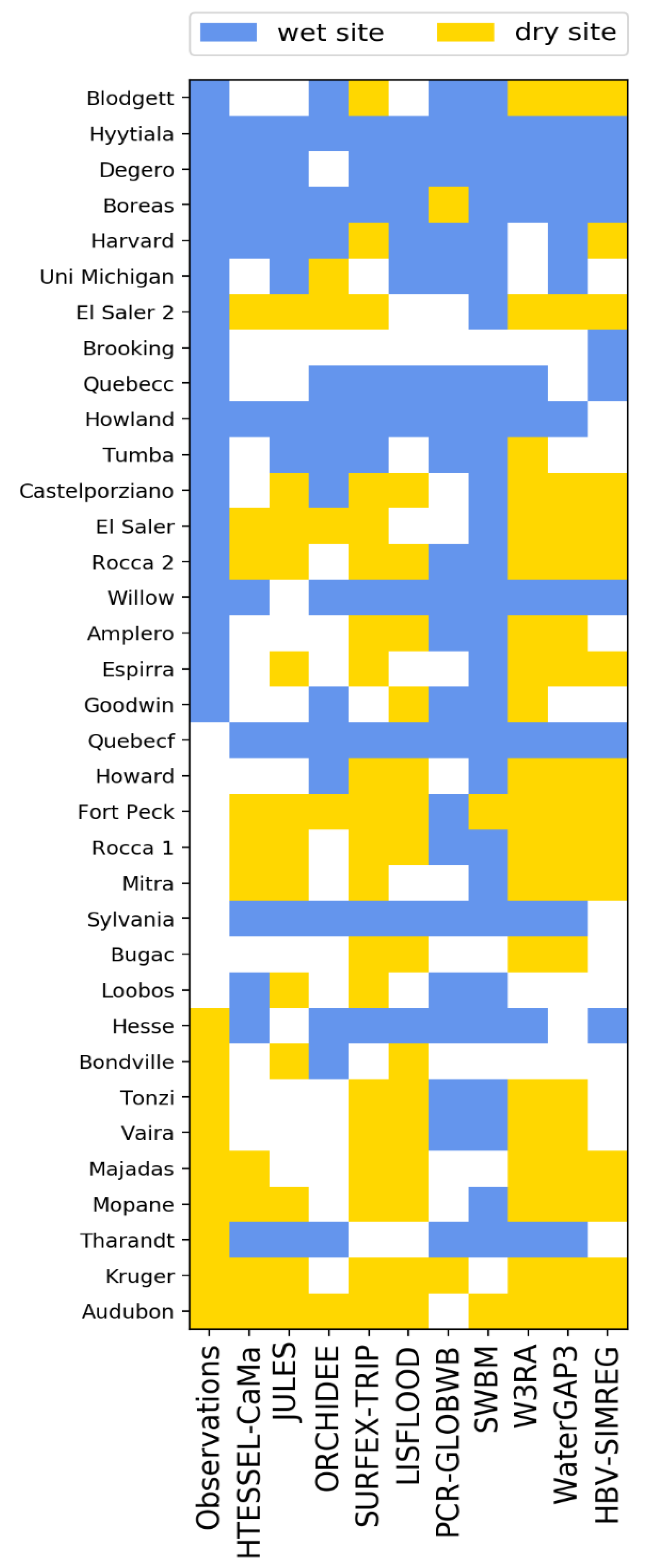
3.1. Site Level Results and Selection of Representative Sites
- Too wet for analysis.
- Observations are too wet, but models are dry enough.
- Both observations and models are dry enough.
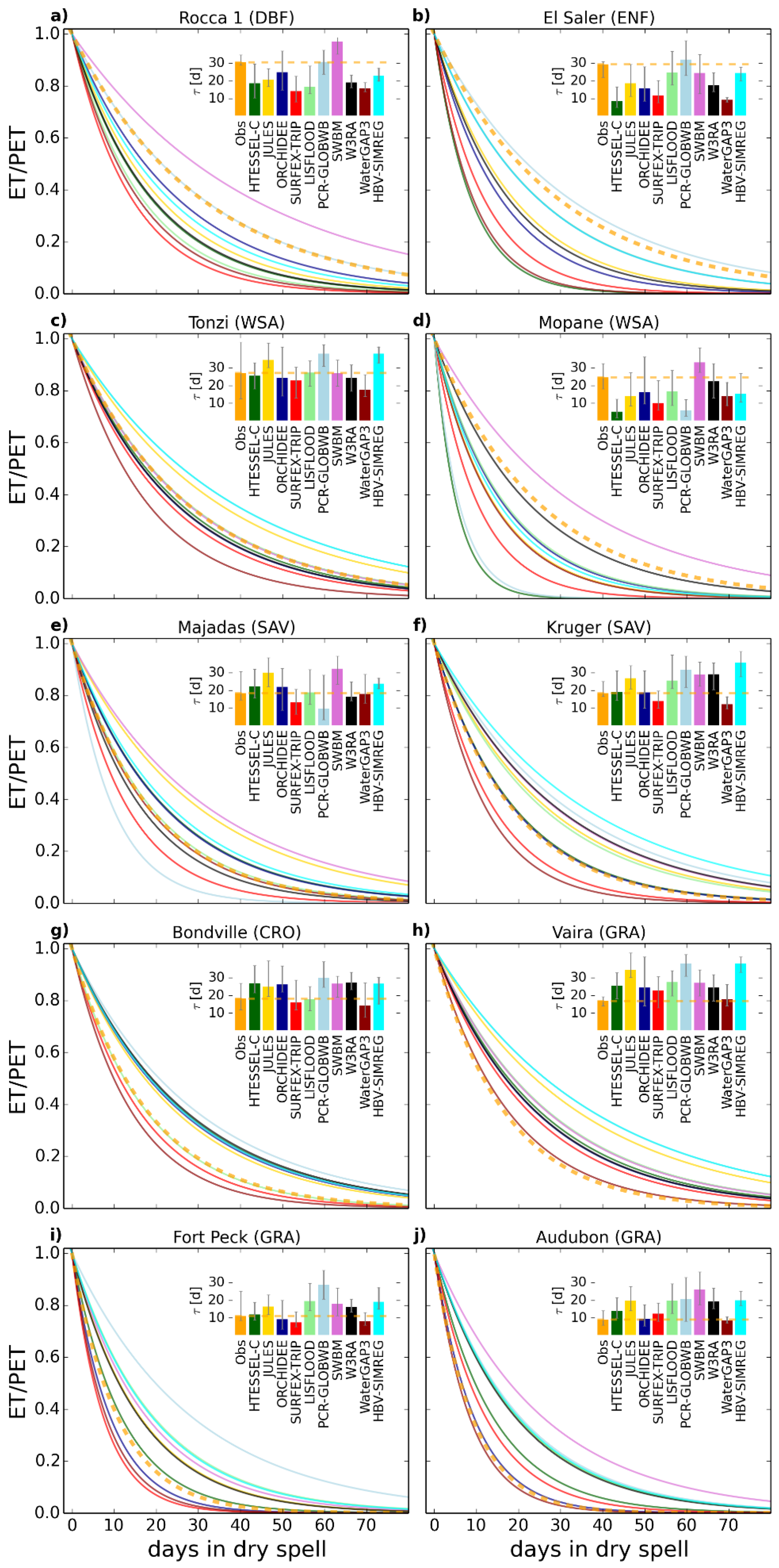
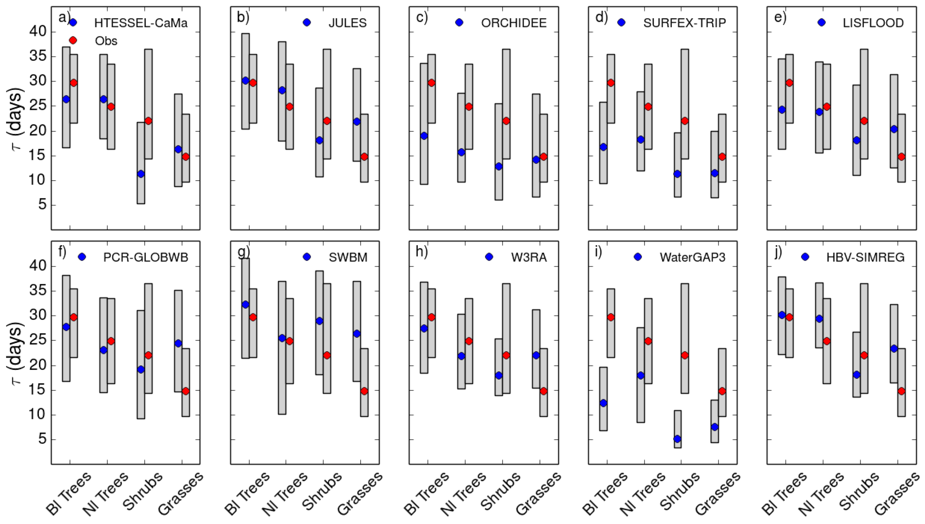
3.2. Analysis of Results at the Site Level
3.3. Generalizing the Results for Model Evaluation
4. Discussion
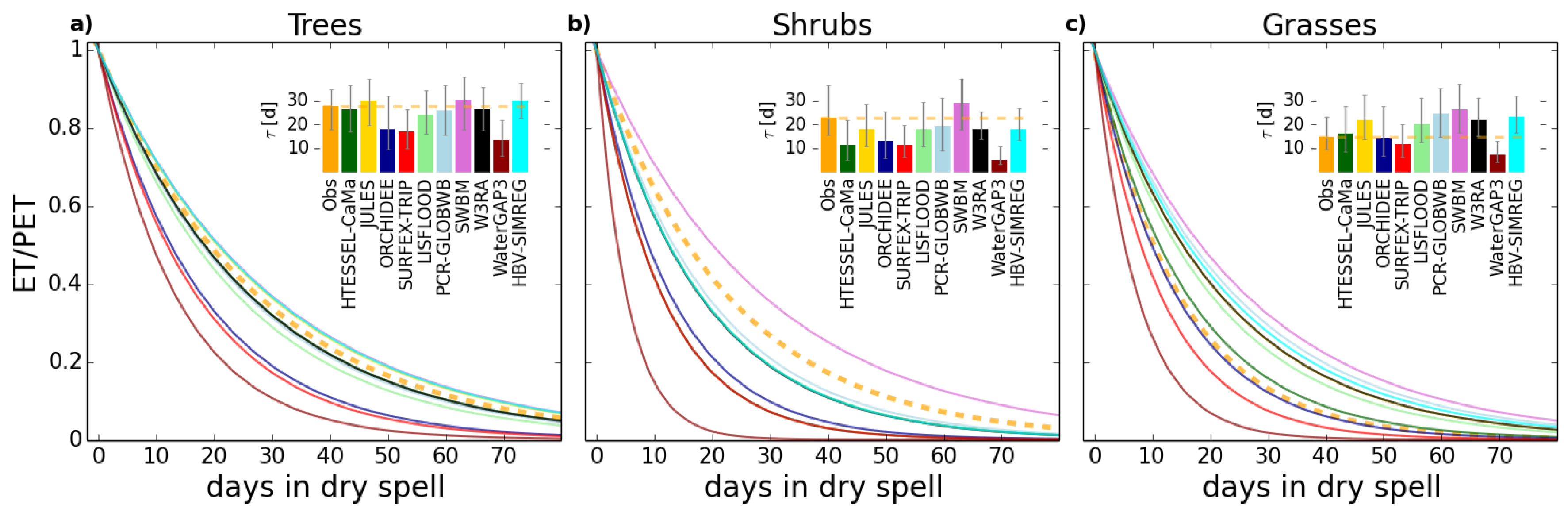
4.1. Role of Vegetation in τ
4.2. Other Factors
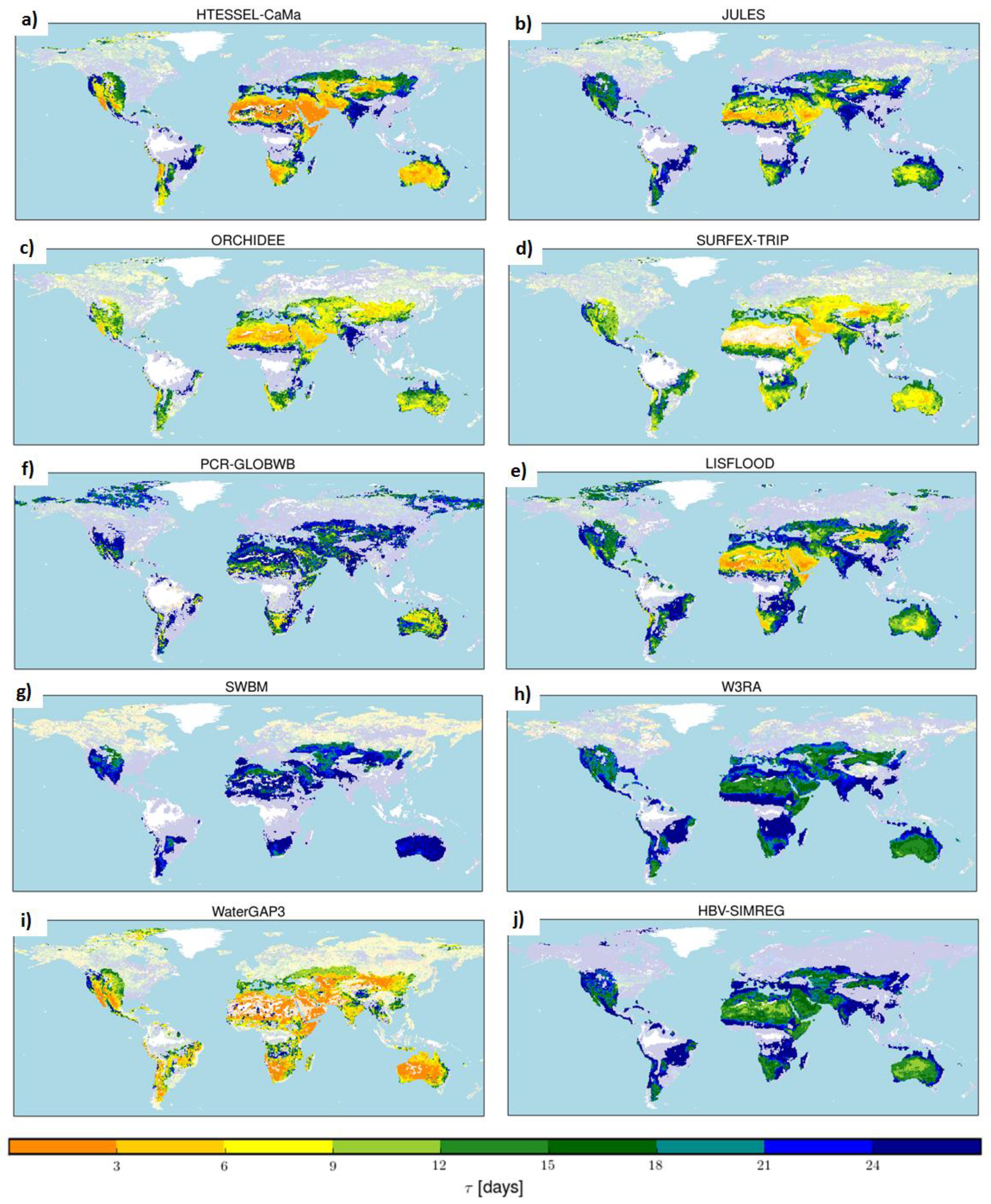
4.3. Global Maps of Median τ
4.4. Identification of Drydowns and Characterization of Sites
4.5. On the Methodolody
5. Summary and Conclusions
Supplementary Materials
Author Contributions
Funding
Acknowledgments
Conflicts of Interest
References
- Seneviratne, S.I.; Corti, T.; Davin, E.L.; Hirschi, M.; Jaeger, E.B.; Lehner, I.; Orlowsky, B.; Teuling, A.J. Investigating soil moisture–climate interactions in a changing climate: A review. Earth-Sci. Rev. 2010, 99, 125–161. [Google Scholar] [CrossRef]
- Botter, G.; Peratoner, F.; Porporato, A.; Rodriguez-Iturbe, I.; Rinaldo, A. Signatures of large-scale soil moisture dynamics on streamflow statistics across U.S. climate regimes. Water Resour. Res. 2007, 43. [Google Scholar] [CrossRef] [Green Version]
- Clark, M.P.; Fan, Y.; Lawrence, D.M.; Adam, J.C.; Bolster, D.; Gochis, D.J.; Hooper, R.P.; Kumar, M.; Leung, L.R.; Mackay, D.S.; et al. Improving the representation of hydrologic processes in Earth System Models. Water Resour. Res. 2015, 51, 5929–5956. [Google Scholar] [CrossRef] [Green Version]
- McColl, K.A.; Alemohammad, S.H.; Akbar, R.; Konings, A.G.; Yueh, S.; Entekhabi, D. The global distribution and dynamics of surface soil moisture. Nat. Geosci. 2017, 10, 100–104. [Google Scholar] [CrossRef]
- Miguez-Macho, G.; Fan, Y. The role of groundwater in the Amazon water cycle: 1. Influence on seasonal streamflow, flooding and wetlands. J. Geophys. Res. Atmos. 2012, 117. [Google Scholar] [CrossRef] [Green Version]
- Rosenzweig, C.; Tubiello, F.N.; Goldberg, R.; Mills, E.; Bloomfield, J. Increased crop damage in the US from excess precipitation under climate change. Glob. Environ. Change 2002, 12, 197–202. [Google Scholar] [CrossRef] [Green Version]
- Teuling, A.J.; Seneviratne, S.I.; Williams, C.; Troch, P.A. Observed timescales of evapotranspiration response to soil moisture. Geophys. Res. Lett. 2006, 33. [Google Scholar] [CrossRef] [Green Version]
- Koster, R.D.; Suarez, M.J. Soil Moisture Memory in Climate Models. J. Hydrometeorol. 2001, 2, 558–570. [Google Scholar] [CrossRef] [Green Version]
- Lorenz, R.; Jaeger, E.B.; Seneviratne, S.I. Persistence of heat waves and its link to soil moisture memory. Geophys. Res. Lett. 2010, 37. [Google Scholar] [CrossRef] [Green Version]
- Taylor, C.M.; de Jeu, R.A.M.; Guichard, F.; Harris, P.P.; Dorigo, W.A. Afternoon rain more likely over drier soils. Nature 2012, 489, 423–426. [Google Scholar] [CrossRef] [Green Version]
- Prudhomme, C.; Giuntoli, I.; Robinson, E.L.; Clark, D.B.; Arnell, N.W.; Dankers, R.; Fekete, B.M.; Franssen, W.; Gerten, D.; Gosling, S.N.; et al. Hydrological droughts in the 21st century, hotspots and uncertainties from a global multimodel ensemble experiment. Proc. Natl. Acad. Sci. USA 2014, 111, 3262–3267. [Google Scholar] [CrossRef]
- Koster, R.D.; Guo, Z.; Yang, R.; Dirmeyer, P.A.; Mitchell, K.; Puma, M.J. On the Nature of Soil Moisture in Land Surface Models. J. Clim. 2009, 22, 4322–4335. [Google Scholar] [CrossRef] [Green Version]
- Best, M.J.; Pryor, M.; Clark, D.B.; Rooney, G.G.; Essery, R.L.H.; Ménard, C.B.; Edwards, J.M.; Hendry, M.A.; Porson, A.; Gedney, N.; et al. The Joint UK Land Environment Simulator (JULES), model description—Part 1: Energy and water fluxes. Geosci. Model Dev. 2011, 4, 677–699. [Google Scholar] [CrossRef]
- Famiglietti, J.S.; Ryu, D.; Berg, A.A.; Rodell, M.; Jackson, T.J. Field observations of soil moisture variability across scales. Water Resour. Res. 2008, 44. [Google Scholar] [CrossRef]
- Entekhabi, D.; Njoku, E.G.; O’Neill, P.E.; Kellogg, K.H.; Crow, W.T.; Edelstein, W.N.; Entin, J.K.; Goodman, S.D.; Jackson, T.J.; Johnson, J.; et al. The Soil Moisture Active Passive (SMAP) Mission. Proc. IEEE 2010, 98, 704–716. [Google Scholar] [CrossRef]
- Kerr, Y.H.; Waldteufel, P.; Richaume, P.; Wigneron, J.P.; Ferrazzoli, P.; Mahmoodi, A.; Bitar, A.A.; Cabot, F.; Gruhier, C.; Juglea, S.E.; et al. The SMOS Soil Moisture Retrieval Algorithm. IEEE Trans. Geosci. Remote Sens. 2012, 50, 1348–1403. [Google Scholar] [CrossRef]
- Liu, Y.Y.; Dorigo, W.A.; Parinussa, R.M.; de Jeu, R.A.M.; Wagner, W.; McCabe, M.F.; Evans, J.P.; van Dijk, A.I.J.M. Trend-preserving blending of passive and active microwave soil moisture retrievals. Remote Sens. Environ. 2012, 123, 280–297. [Google Scholar] [CrossRef]
- Albergel, C.; de Rosnay, P.; Gruhier, C.; Muñoz-Sabater, J.; Hasenauer, S.; Isaksen, L.; Kerr, Y.; Wagner, W. Evaluation of remotely sensed and modelled soil moisture products using global ground-based in situ observations. Remote Sens. Environ. 2012, 118, 215–226. [Google Scholar] [CrossRef]
- Champagne, C.; Rowlandson, T.; Berg, A.; Burns, T.; L’Heureux, J.; Tetlock, E.; Adams, J.R.; McNairn, H.; Toth, B.; Itenfisu, D. Satellite surface soil moisture from SMOS and Aquarius: Assessment for applications in agricultural landscapes. Int. J. Appl. Earth Obs. Geoinf. 2016, 45, 143–154. [Google Scholar] [CrossRef] [Green Version]
- McColl, K.A.; Wang, W.; Peng, B.; Akbar, R.; Short Gianotti, D.J.; Lu, H.; Pan, M.; Entekhabi, D. Global characterization of surface soil moisture drydowns. Geophys. Res. Lett. 2017, 44, 3682–3690. [Google Scholar] [CrossRef]
- Shellito, P.J.; Small, E.E.; Colliander, A.; Bindlish, R.; Cosh, M.H.; Berg, A.A.; Bosch, D.D.; Caldwell, T.G.; Goodrich, D.C.; McNairn, H.; et al. SMAP soil moisture drying more rapid than observed in situ following rainfall events. Geophys. Res. Lett. 2016, 43, 8068–8075. [Google Scholar] [CrossRef] [Green Version]
- Shellito, P.J.; Small, E.E.; Livneh, B. Controls on surface soil drying rates observed by SMAP and simulated by the Noah land surface model. Hydrol. Earth Syst. Sci. 2018, 22, 1649–1663. [Google Scholar] [CrossRef] [Green Version]
- Ghannam, K.; Nakai, T.; Paschalis, A.; Oishi, C.A.; Kotani, A.; Igarashi, Y.; Kumagai, T.O.; Katul, G.G. Persistence and memory timescales in root-zone soil moisture dynamics. Water Resour. Res. 2016, 52, 1427–1445. [Google Scholar] [CrossRef] [Green Version]
- Orth, R.; Seneviratne, S.I. Analysis of soil moisture memory from observations in Europe. J. Geophys. Res. Atmos. 2012, 117. [Google Scholar] [CrossRef] [Green Version]
- Dirmeyer, P.A.; Wu, J.; Norton, H.E.; Dorigo, W.A.; Quiring, S.M.; Ford, T.W.; Santanello, J.A., Jr.; Bosilovich, M.G.; Ek, M.B.; Koster, R.D.; et al. Confronting Weather and Climate Models with Observational Data from Soil Moisture Networks over the United States. J. Hydrometeorol. 2016, 17, 1049–1067. [Google Scholar] [CrossRef]
- Blyth, E.; Harding, R.J. Methods to separate observed global evapotranspiration into the interception, transpiration and soil surface evaporation components. Hydrol. Process. 2011, 25, 4063–4068. [Google Scholar] [CrossRef]
- Laio, F.; Porporato, A.; Ridolfi, L.; Rodriguez-Iturbe, I. Plants in water-controlled ecosystems: Active role in hydrologic processes and response to water stress: II. Probabilistic soil moisture dynamics. Adv. Water Resour. 2001, 24, 707–723. [Google Scholar] [CrossRef]
- Harris, P.P.; Folwell, S.S.; Gallego-Elvira, B.; Rodríguez, J.; Milton, S.; Taylor, C.M. An Evaluation of Modeled Evaporation Regimes in Europe Using Observed Dry Spell Land Surface Temperature. J. Hydrometeorol. 2017, 18, 1453–1470. [Google Scholar] [CrossRef]
- Folwell, S.S.; Harris, P.P.; Taylor, C.M. Large-Scale Surface Responses during European Dry Spells Diagnosed from Land Surface Temperature. J. Hydrometeorol. 2016, 17, 975–993. [Google Scholar] [CrossRef]
- Gallego-Elvira, B.; Taylor, C.M.; Harris, P.P.; Ghent, D.; Veal, K.L.; Folwell, S.S. Global observational diagnosis of soil moisture control on the land surface energy balance. Geophys. Res. Lett. 2016, 43, 2623–2631. [Google Scholar] [CrossRef] [Green Version]
- Blyth, E.; Gash, J.; Lloyd, A.; Pryor, M.; Weedon, G.P.; Shuttleworth, J. Evaluating the JULES Land Surface Model Energy Fluxes Using FLUXNET Data. J. Hydrometeorol. 2010, 11, 509–519. [Google Scholar] [CrossRef] [Green Version]
- Abramowitz, G. Towards a public, standardized, diagnostic benchmarking system for land surface models. Geosci. Model Dev. 2012, 5, 819–827. [Google Scholar] [CrossRef] [Green Version]
- Abramowitz, G.; Pouyanné, L.; Ajami, H. On the information content of surface meteorology for downward atmospheric long-wave radiation synthesis. Geophys. Res. Lett. 2012, 39. [Google Scholar] [CrossRef] [Green Version]
- Schellekens, J.; Dutra, E.; Martínez-de la Torre, A.; Balsamo, G.; van Dijk, A.; Sperna Weiland, F.; Minvielle, M.; Calvet, J.C.; Decharme, B.; Eisner, S.; et al. A global water resources ensemble of hydrological models: The eartH2Observe Tier-1 dataset. Earth Syst. Sci. Data 2017, 9, 389–413. [Google Scholar] [CrossRef]
- Weedon, G.P.; Balsamo, G.; Bellouin, N.; Gomes, S.; Best, M.J.; Viterbo, P. The WFDEI meteorological forcing data set: WATCH Forcing Data methodology applied to ERA-Interim reanalysis data. Water Resour. Res. 2014, 50, 7505–7514. [Google Scholar] [CrossRef] [Green Version]
- Balsamo, G.; Beljaars, A.; Scipal, K.; Viterbo, P.; Hurk, B.V.D.; Hirschi, M.; Betts, A.K. A Revised Hydrology for the ECMWF Model: Verification from Field Site to Terrestrial Water Storage and Impact in the Integrated Forecast System. J. Hydrometeorol. 2009, 10, 623–643. [Google Scholar] [CrossRef]
- Clark, D.B.; Mercado, L.M.; Sitch, S.; Jones, C.D.; Gedney, N.; Best, M.J.; Pryor, M.; Rooney, G.G.; Essery, R.L.H.; Blyth, E.; et al. The Joint UK Land Environment Simulator (JULES), model description—Part 2: Carbon fluxes and vegetation dynamics. Geosci. Model Dev. 2011, 4, 701–722. [Google Scholar] [CrossRef]
- Barella-Ortiz, A.; Polcher, J.; Tuzet, A.; Laval, K. Potential evaporation estimation through an unstressed surface-energy balance and its sensitivity to climate change. Hydrol. Earth Syst. Sci. 2013, 17, 4625–4639. [Google Scholar] [CrossRef] [Green Version]
- d’Orgeval, T.; Polcher, J.; de Rosnay, P. Sensitivity of the West African hydrological cycle in ORCHIDEE to infiltration processes. Hydrol. Earth Syst. Sci. 2008, 12, 1387–1401. [Google Scholar] [CrossRef] [Green Version]
- Krinner, G.; Viovy, N.; de Noblet-Ducoudré, N.; Ogée, J.; Polcher, J.; Friedlingstein, P.; Ciais, P.; Sitch, S.; Prentice, I.C. A dynamic global vegetation model for studies of the coupled atmosphere-biosphere system. Glob. Biogeochem. Cycles 2005, 19. [Google Scholar] [CrossRef] [Green Version]
- Decharme, B.; Martin, E.; Faroux, S. Reconciling soil thermal and hydrological lower boundary conditions in land surface models. J. Geophys. Res. Atmos. 2013, 118, 7819–7834. [Google Scholar] [CrossRef] [Green Version]
- Decharme, B.; Alkama, R.; Douville, H.; Becker, M.; Cazenave, A. Global Evaluation of the ISBA-TRIP Continental Hydrological System. Part II: Uncertainties in River Routing Simulation Related to Flow Velocity and Groundwater Storage. J. Hydrometeorol. 2010, 11, 601–617. [Google Scholar] [CrossRef] [Green Version]
- Van Der Knijff, J.M.; Younis, J.; De Roo, A.P.J. LISFLOOD: A GIS-based distributed model for river basin scale water balance and flood simulation. Int. J. Geogr. Inf. Sci. 2010, 24, 189–212. [Google Scholar] [CrossRef]
- Van Beek, L.P.H.; Bierkens, M.F.P. The Global Hydrological Model PCR-GLOBWB: Conceptualization, Parameterization and Verification; Department of Physical Geography, Utrecht University: Utrecht, The Netherlands, 2008; Available online: http://vanbeek.geo.uu.nl/suppinfo/vanbeekbierkens2009.pdf (accessed on 19 February 2019).
- Van Beek, L.P.H.; Wada, Y.; Bierkens, M.F.P. Global monthly water stress: 1. Water balance and water availability. Water Resour. Res. 2011, 47. [Google Scholar] [CrossRef] [Green Version]
- Wada, Y.; Wisser, D.; Bierkens, M.F.P. Global modeling of withdrawal, allocation and consumptive use of surface water and groundwater resources. Earth Syst. Dyn. 2014, 5, 15–40. [Google Scholar] [CrossRef] [Green Version]
- Orth, R.; Seneviratne, S.I. Predictability of soil moisture and streamflow on subseasonal timescales: A case study. J. Geophys. Res. Atmos. 2013, 118, 10963–10979. [Google Scholar] [CrossRef]
- Van Dijk, A.I.J.M.; Renzullo, L.J.; Wada, Y.; Tregoning, P. A global water cycle reanalysis (2003–2012) merging satellite gravimetry and altimetry observations with a hydrological multi-model ensemble. Hydrol. Earth Syst. Sci. 2014, 18, 2955–2973. [Google Scholar] [CrossRef] [Green Version]
- Van Dijk, A.I.J.M.; Warren, G. The Australian Water Resources Assessment System; Technical Report 4; Landscape Model (version 0.5) Evaluation Against Observations; CSIRO: Water for a Healthy Country National Research Flagship: Canberra, Australia, 2010.
- Döll, P.; Fiedler, K.; Zhang, J. Global-scale analysis of river flow alterations due to water withdrawals and reservoirs. Hydrol. Earth Syst. Sci. 2009, 13, 2413–2432. [Google Scholar] [CrossRef] [Green Version]
- Flörke, M.; Kynast, E.; Bärlund, I.; Eisner, S.; Wimmer, F.; Alcamo, J. Domestic and industrial water uses of the past 60 years as a mirror of socio-economic development: A global simulation study. Glob. Environ. Chang. 2013, 23, 144–156. [Google Scholar] [CrossRef]
- Beck, H.E.; van Dijk, A.I.J.M.; de Roo, A.; Miralles, D.G.; McVicar, T.R.; Schellekens, J.; Bruijnzeel, L.A. Global-scale regionalization of hydrologic model parameters. Water Resour. Res. 2016, 52, 3599–3622. [Google Scholar] [CrossRef] [Green Version]
- Lindström, G.; Johansson, B.; Persson, M.; Gardelin, M.; Bergström, S. Development and test of the distributed HBV-96 hydrological model. J. Hydrol. 1997, 201, 272–288. [Google Scholar] [CrossRef]
- Miguez-Macho, G.; Fan, Y. The role of groundwater in the Amazon water cycle: 2. Influence on seasonal soil moisture and evapotranspiration. J. Geophys. Res. Atmos. 2012, 117. [Google Scholar] [CrossRef] [Green Version]
- Ukkola, A.M.; Kauwe, M.G.D.; Pitman, A.J.; Best, M.J.; Abramowitz, G.; Haverd, V.; Decker, M.; Haughton, N. Land surface models systematically overestimate the intensity, duration and magnitude of seasonal-scale evaporative droughts. Environ. Res. Lett. 2016, 11, 104012. [Google Scholar] [CrossRef] [Green Version]
- Monteith, J.L. Evaporation and the Environment in the State and Movement of Water in Living Organisms. In Proceedings of the Society for Experimental Biology, Symposium No. 19; Cambridge University Press: Cambridge, UK, 1965; pp. 205–234. [Google Scholar]
- Robinson, E.L.; Blyth, E.M.; Clark, D.B.; Finch, J.; Rudd, A.C. Trends in atmospheric evaporative demand in Great Britain using high-resolution meteorological data. Hydrol. Earth Syst. Sci. 2017, 21, 1189–1224. [Google Scholar] [CrossRef] [Green Version]
- Chen, B.; Coops, N.C.; Fu, D.; Margolis, H.A.; Amiro, B.D.; Barr, A.G.; Black, T.A.; Arain, M.A.; Bourque, C.P.A.; Flanagan, L.B.; et al. Assessing eddy-covariance flux tower location bias across the Fluxnet-Canada Research Network based on remote sensing and footprint modelling. Agric. For. Meteorol. 2011, 151, 87–100. [Google Scholar] [CrossRef] [Green Version]
- Baldocchi, D.D.; Xu, L. What limits evaporation from Mediterranean oak woodlands—The supply of moisture in the soil, physiological control by plants or the demand by the atmosphere? Adv. Water Resour. 2007, 30, 2113–2122. [Google Scholar] [CrossRef]
- Blyth, E.; Clark, D.B.; Ellis, R.; Huntingford, C.; Los, S.; Pryor, M.; Best, M.; Sitch, S. A comprehensive set of benchmark tests for a land surface model of simultaneous fluxes of water and carbon at both the global and seasonal scale. Geosci. Model Dev. 2011, 4, 255–269. [Google Scholar] [CrossRef] [Green Version]
- FAO/IIASA/ISRIC/ISS-CAS/JRC. Harmonized World Soil Database (version 1.2); FAO: Rome, Italy; IIASA: Laxenburg, Austria, 2012. [Google Scholar]
- Miguez-Macho, G.; Fan, Y.; Weaver, C.P.; Walko, R.; Robock, A. Incorporating water table dynamics in climate modeling: 2. Formulation, validation, and soil moisture simulation. J. Geophys. Res. Atmos. 2007, 112. [Google Scholar] [CrossRef] [Green Version]


| Site | Country | Latitude | Longitude | Vegetation Type | Period of Data |
|---|---|---|---|---|---|
| Amplero | Italy | 41.90° N | 13.61° E | Grassland | 2003–2006 |
| Audubon | United States | 31.59° N | 110.51° W | Grassland | 2003–2005 |
| Blodgett | United States | 38.90° N | 120.63° W | Evergreen Needleleaf | 2000–2006 |
| Bondville | United States | 40.01° N | 88.29° W | Cropland | 1997–2006 |
| Boreas | Canada | 55.88° N | 98.48° W | Evergreen Needleleaf | 1997–2003 |
| Brooking | United States | 44.35° N | 96.84° W | Grassland | 2005–2006 |
| Bugac | Hungary | 46.69° N | 19.60° E | Grassland | 2003–2006 |
| Castelporziano | Italy | 41.71° N | 12.38° E | Evergreen Broadleaf | 2001–2006 |
| Degero | Sweden | 64.18° N | 19.55° E | Permanent Wetland | 2001–2005 |
| El Saler | Spain | 39.35° N | 0.32° W | Evergreen Needleleaf | 1999–2006 |
| El Saler 2 | Spain | 39.28° N | 0.32° W | Cropland | 2005–2006 |
| Espirra | Portugal | 38.64° N | 8.60° W | Evergreen Broadleaf | 2002–2006 |
| Fort Peck | United States | 48.31° N | 105.10° W | Grassland | 2000–2006 |
| Goodwin | United States | 34.25° N | 89.87° W | Grassland | 2004–2006 |
| Harvard | United States | 42.54° N | 72.17° W | Deciduous Broadleaf | 1994–2001 |
| Hesse | France | 48.67° N | 7.06° E | Deciduous Needleleaf | 2001–2006 |
| Howard | Australia | 12.49° S | 131.15° E | Woody Savanna | 2002–2005 |
| Howland | United States | 45.20° N | 68.74° W | Evergreen Needleleaf | 1996–2004 |
| Hyytiala | Finland | 61.85° N | 24.29° E | Evergreen Needleleaf | 2001–2004 |
| Kruger | South Africa | 25.02° S | 31.50° E | Savanna | 2002–2003 |
| Loobos | Netherlands | 52.17° N | 5.74° E | Evergreen Needleleaf | 1997–2006 |
| Majadas | Spain | 39.94° N | 5.77° W | Savanna | 2004–2006 |
| Mitra | Portugal | 38.54° N | 8.00° W | Evergreen Broadleaf | 2005–2005 |
| Mopane | Botswana | 19.92° S | 23.56° E | Woody Savanna | 1999–2001 |
| Quebecc | Canada | 49.27° N | 74.04° W | Evergreen Needleleaf | 2002–2006 |
| Quebecf | Canada | 49.69° N | 74.34° W | Evergreen Needleleaf | 2004–2006 |
| Rocca 1 | Italy | 42.41° N | 11.93° E | Deciduous Broadleaf | 2002–2006 |
| Rocca 2 | Italy | 42.39° N | 11.92° E | Deciduous Broadleaf | 2004–2006 |
| Sylvania | United States | 46.24° N | 89.35° W | Mixed Forest | 2002–2005 |
| Tharandt | Germany | 50.96° N | 13.57° E | Evergreen Needleleaf | 1998–2005 |
| Tonzi | United States | 38.43° N | 120.97° W | Woody Savanna | 2002–2006 |
| Tumba | Australia | 35.66° S | 148.15° E | Evergreen Broadleaf | 2002–2005 |
| Uni Michigan | United States | 45.56° N | 84.71° W | Deciduous Broadleaf | 1999–2003 |
| Vaira | United States | 38.41° N | 120.95° W | Grassland | 2001–2006 |
| Willow | United States | 45.81° N | 90.01° W | Deciduous Broadleaf | 1999–2006 |
| Model | Type | Time Step | Evapotranspiration Scheme | Soil Layers | Groundwater Interactions | References |
|---|---|---|---|---|---|---|
| HTESSEL-CaMa | LSM | 1 h | Penman–Monteith | 4 | No | [36] |
| JULES | LSM | 1 h | Penman–Monteith | 4 | No | [13,37] |
| ORCHIDEE | LSM | 900 s | Bulk PET [38] | 11 | No | [39,40] |
| SURFEX-TRIP | LSM | 900 s | Penman–Monteith | 14 | No | [41,42] |
| LISFLOOD | GHM | 1 day | Penman–Monteith | 2 | No | [43] |
| PCR-GLOBWB | GHM | 1 day | Hamon (tier 1) or imposed as forcing | 1 | Yes | [44,45,46] |
| SWBM | GHM | 1 day | Inferred from net radiation | 1 | No | [47] |
| W3RA | GHM | 1 day | Penman–Monteith | 3 | Yes | [48,49] |
| WaterGAP3 | GHM | 1 day | Priestley–Taylor | 1 | No | [50,51] |
| HBV-SIMREG | GHM | 1 day | Penman, 1948 | 1 | No | [52,53] |
| Site | τ [d] | Ndry | IQR [d] | Ndry/Ntotal |
|---|---|---|---|---|
| Blodgett | 14.2 | 1 | -- | 0.04 |
| Hyytiala | 40.8 | 1 | -- | 0.09 |
| Degero | 45 | 1 | -- | 0.09 |
| Boreas | 32.9 | 1 | -- | 0.11 |
| Harvard | 23.1 | 1 | -- | 0.13 |
| Uni Michigan | 12.4 | 1 | -- | 0.13 |
| El Saler 2 | 34.6 | 2 | 2.5 | 0.13 |
| Brooking | 14.2 | 1 | -- | 0.14 |
| Quebecc | 8.1 | 1 | -- | 0.17 |
| Howlandm | 33.3 | 2 | 15.2 | 0.18 |
| Tumba | 37.6 | 2 | 7.6 | 0.18 |
| Castel | 38.0 | 2 | 10.6 | 0.18 |
| El Saler | 29.3 | 7 | 8.9 | 0.2 |
| Rocca 2 | 35.8 | 2 | 3.1 | 0.22 |
| Willow | 17.9 | 3 | 3.9 | 0.23 |
| Amplero | 17.6 | 1 | -- | 0.25 |
| Espirra | 28.6 | 3 | 6.8 | 0.25 |
| Goodwin | 19.2 | 2 | 4.6 | 0.25 |
| Quebecf | 16.8 | 2 | 8.2 | 0.29 |
| Howard | 25.5 | 4 | 10.2 | 0.33 |
| Fort Peck | 10.9 | 8 | 16.4 | 0.35 |
| Rocca 1 | 30.5 | 7 | 6.0 | 0.37 |
| Mitra | 35.8 | 3 | 3.6 | 0.38 |
| Sylvania | 17.9 | 2 | 5.6 | 0.4 |
| Bugac | 28.5 | 3 | 8.5 | 0.43 |
| Loobos | 16.2 | 5 | 6.2 | 0.45 |
| Hesse | 23.4 | 5 | 4.7 | 0.5 |
| Bondville | 18.2 | 10 | 15.2 | 0.5 |
| Tonzi | 27.1 | 12 | 32.2 | 0.5 |
| Vaira | 16.8 | 13 | 5.2 | 0.54 |
| Majadas | 18.4 | 11 | 16.1 | 0.58 |
| Mopane | 24.7 | 12 | 14.3 | 0.75 |
| Tharandt | 29.2 | 4 | 13.4 | 0.8 |
| Kruger | 18.4 | 9 | 8.5 | 0.82 |
| Audubon | 9.1 | 16 | 8.4 | 0.94 |
| Site | Observations | HTESSEL-CaMa | JULES | ORCHIDEE | SURFEX-TRIP | LISFLOOD | PCR-GLOBWB | SWBM | W3RA | WaterGAP3 | HBV-SIMREG |
|---|---|---|---|---|---|---|---|---|---|---|---|
| Rocca 1 | 30.5 | 18.7 | 20.7 | 25.0 | 14.1 | 16.6 | 30.7 | 42.4 | 19.0 | 15.6 | 22.9 |
| El Saler | 29.3 | 8.7 | 18.7 | 15.7 | 11.7 | 24.6 | 31.9 | 24.6 | 17.6 | 9.2 | 24.5 |
| Tonzi | 27.1 | 25.4 | 34.5 | 24.3 | 22.8 | 27.4 | 37.9 | 27.1 | 24.5 | 17.8 | 38.0 |
| Mopane | 24.7 | 5.2 | 14.1 | 16.3 | 10.2 | 16.7 | 5.9 | 33.1 | 22.3 | 13.9 | 15.2 |
| Majadas | 18.4 | 22.2 | 30.1 | 22.0 | 13.2 | 18.8 | 9.7 | 32.3 | 16.5 | 18.0 | 23.6 |
| Kruger | 18.4 | 19.0 | 26.7 | 18.7 | 14.0 | 25.6 | 31.5 | 28.8 | 29.1 | 12.2 | 35.6 |
| Bondville | 18.2 | 26.8 | 24.9 | 26.9 | 16.2 | 17.9 | 29.9 | 26.7 | 27.3 | 14.3 | 26.6 |
| Vaira | 16.8 | 25.4 | 34.5 | 24.3 | 22.8 | 27.4 | 37.9 | 27.1 | 24.5 | 17.8 | 38.0 |
| Fort Peck | 10.9 | 11.8 | 16.3 | 9.1 | 7.5 | 19.5 | 28.6 | 16.7 | 15.7 | 8.2 | 19.1 |
| Audubon | 9.1 | 14.0 | 19.7 | 9.5 | 12.3 | 19.7 | 19.5 | 25.8 | 19.3 | 8.4 | 20.0 |
| Site | Site Vegetation Type | Grid Cell Dominant PFT |
|---|---|---|
| Rocca 1 | Deciduous Broadleaf | Shrubs |
| El Saler | Evergreen Needleleaf | Grasses |
| Tonzi | Woody Savanna | Broadleaf Trees |
| Mopane | Woody Savanna | Grasses |
| Majadas | Savanna | Grasses |
| Kruger | Savanna | Grasses |
| Bondville | Cropland | Grasses |
| Vaira | Grassland | Broadleaf Trees |
| Fort Peck | Grassland | Grasses |
| Audubon | Grassland | Grasses |
| Observations | HTESSEL-CaMa | JULES | ORCHIDEE | SURFEX-TRIP | LISFLOOD | PCR-GLOBWB | SWBM | W3RA | WaterGAP3 | HBV-SIMREG | |
|---|---|---|---|---|---|---|---|---|---|---|---|
| Trees | 27.8 | 26.4 | 29.7 | 18.1 | 17.1 | 24.2 | 25.8 | 30.1 | 26.3 | 13.4 | 29.9 |
| Grasses | 14.8 | 16.2 | 21.9 | 14.2 | 11.6 | 20.3 | 24.5 | 26.5 | 22.0 | 7.5 | 23.3 |
| % decrease | 47 | 38 | 26 | 21 | 32 | 16 | 5 | 12 | 16 | 44 | 22 |
© 2019 by the authors. Licensee MDPI, Basel, Switzerland. This article is an open access article distributed under the terms and conditions of the Creative Commons Attribution (CC BY) license (http://creativecommons.org/licenses/by/4.0/).
Share and Cite
Martínez-de la Torre, A.; Blyth, E.M.; Robinson, E.L. Evaluation of Drydown Processes in Global Land Surface and Hydrological Models Using Flux Tower Evapotranspiration. Water 2019, 11, 356. https://doi.org/10.3390/w11020356
Martínez-de la Torre A, Blyth EM, Robinson EL. Evaluation of Drydown Processes in Global Land Surface and Hydrological Models Using Flux Tower Evapotranspiration. Water. 2019; 11(2):356. https://doi.org/10.3390/w11020356
Chicago/Turabian StyleMartínez-de la Torre, Alberto, Eleanor M. Blyth, and Emma L. Robinson. 2019. "Evaluation of Drydown Processes in Global Land Surface and Hydrological Models Using Flux Tower Evapotranspiration" Water 11, no. 2: 356. https://doi.org/10.3390/w11020356
APA StyleMartínez-de la Torre, A., Blyth, E. M., & Robinson, E. L. (2019). Evaluation of Drydown Processes in Global Land Surface and Hydrological Models Using Flux Tower Evapotranspiration. Water, 11(2), 356. https://doi.org/10.3390/w11020356