Comparative Study of Hydraulic Simulation Techniques for Water Supply Networks under Earthquake Hazard


Abstract
1. Introduction
2. Methodology
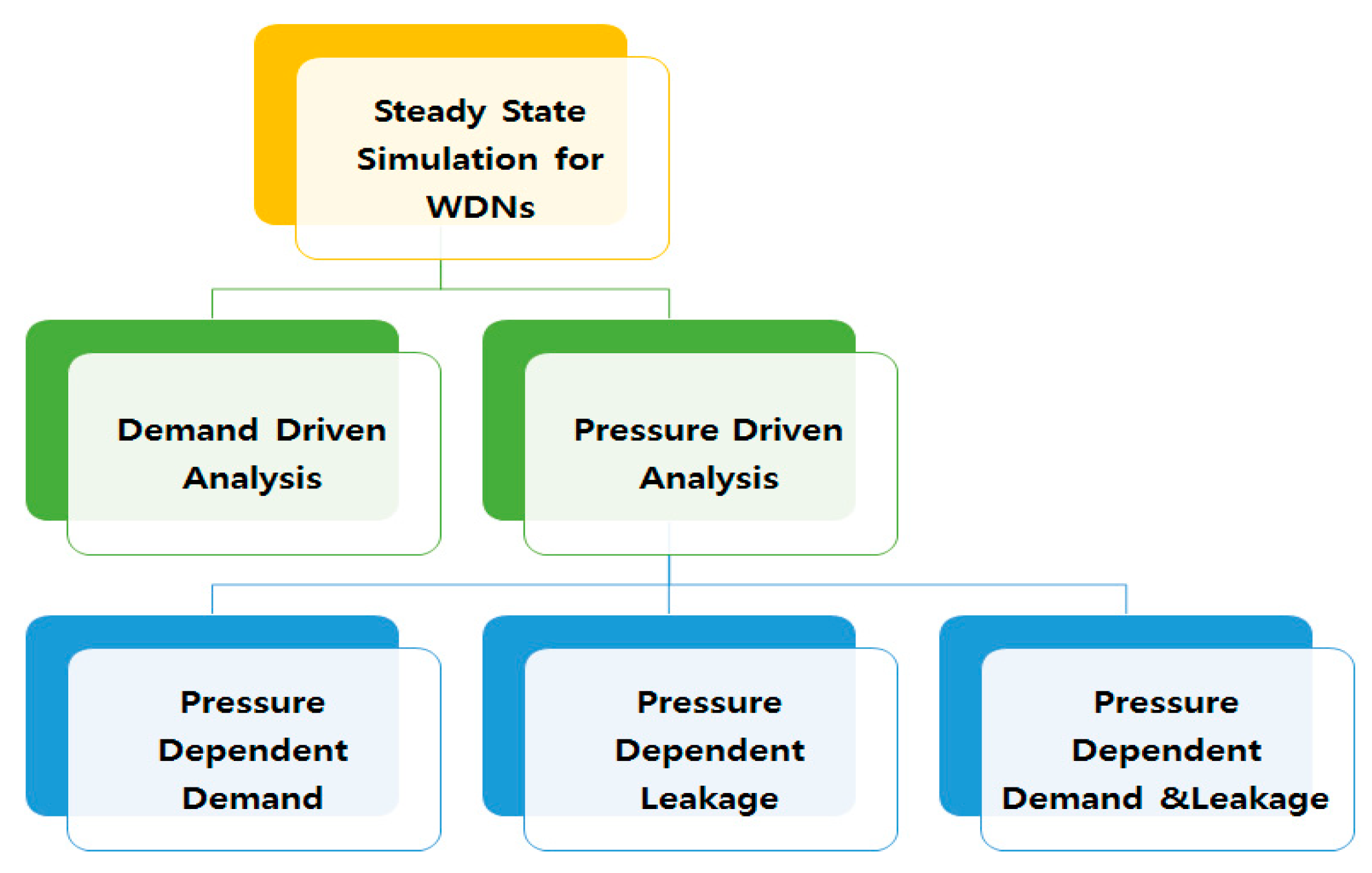
2.1. Pressure Dependent Demand & Leakage (PDDL) Simulation
- (DDA) A technique for calculating the pressure head of a point using continuity equations and cyclic equations under the assumption that demands by demand point are known values and can be supplied always(usage, leakage quantity and so forth, are entered as demands)
- (PDA) A technique to conduct numerical analyses considering the suppliable quantity for each demand node and the leakage quantity of the pipe as pressure dependent factors and as variables that must be determined through pipe network analysis
- (PDD) The available quantity for each node is determined by the head-outflow relationship (HOR) set based on the minimum head and the sufficient head and the head and the suppliable flow rate that are in a non-linear relationship are simultaneously calculated.
- (PDL) This is determined by the relational expression indicating that leakage quantities change according to the pressure head in the pipe (representative relational expression—FAVAD) and simultaneously calculates the pressure head and leakage quantities in the pipe using an expression expressed with a combination of leakage coefficients by pipe and the leakage index.
- (PDDL) A method of analysis considering both PDD and PDL analyses
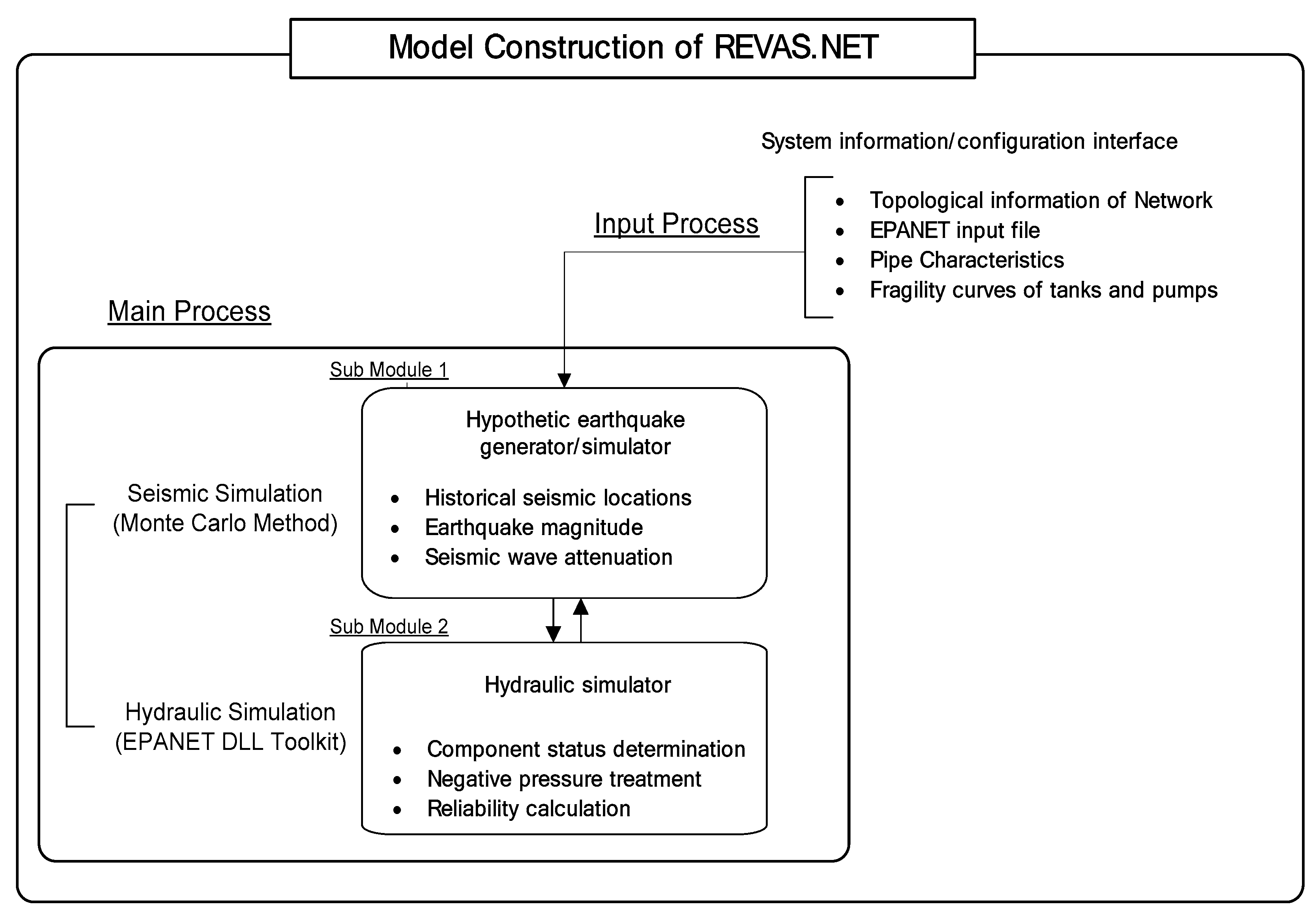
2.2. REVAS.NET
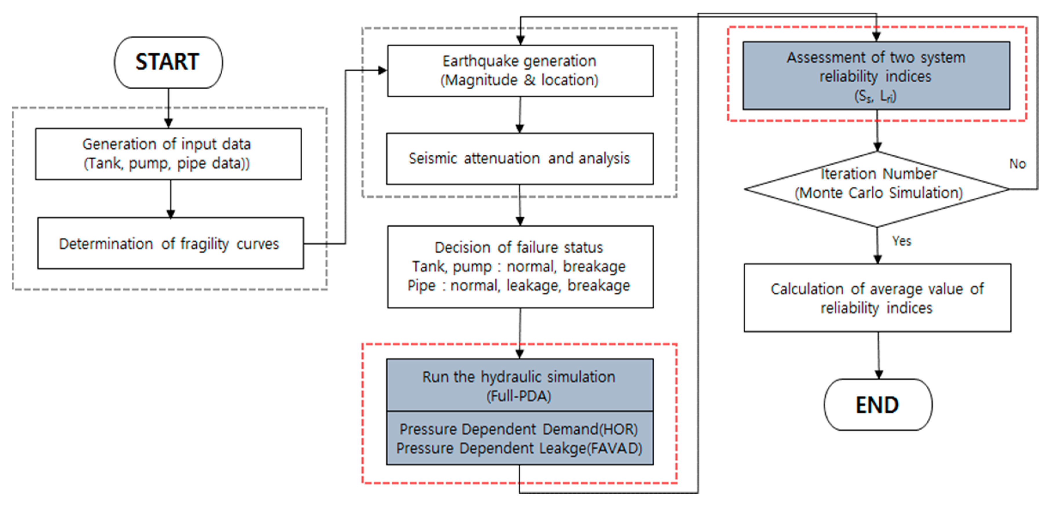
2.3. Proposed Method
2.4. Reliability Quantification Factors
2.4.1. System Serviceability ()
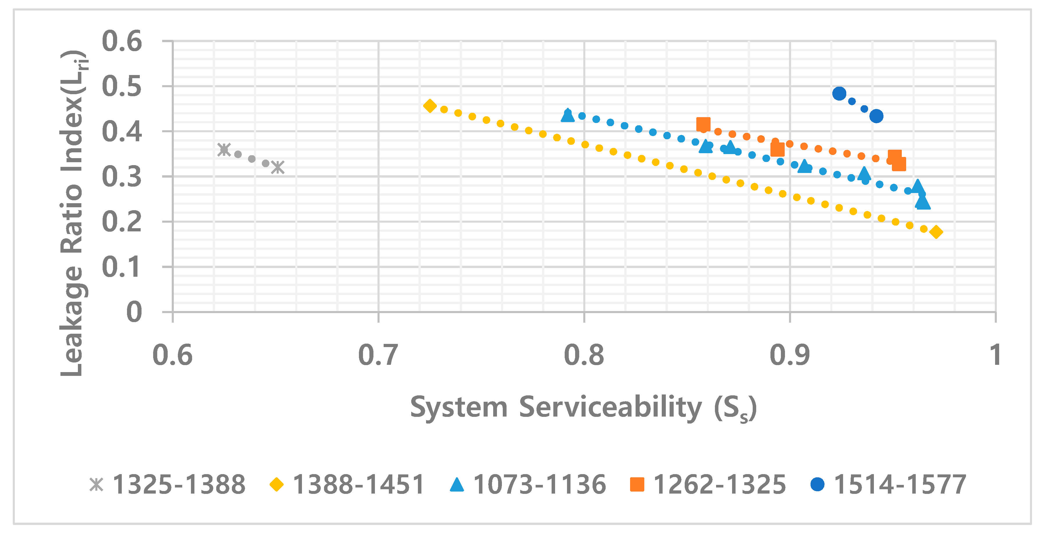
2.4.2. Leakage Ratio Index (Lri)
2.5. Model Configuration
3. Application and Results
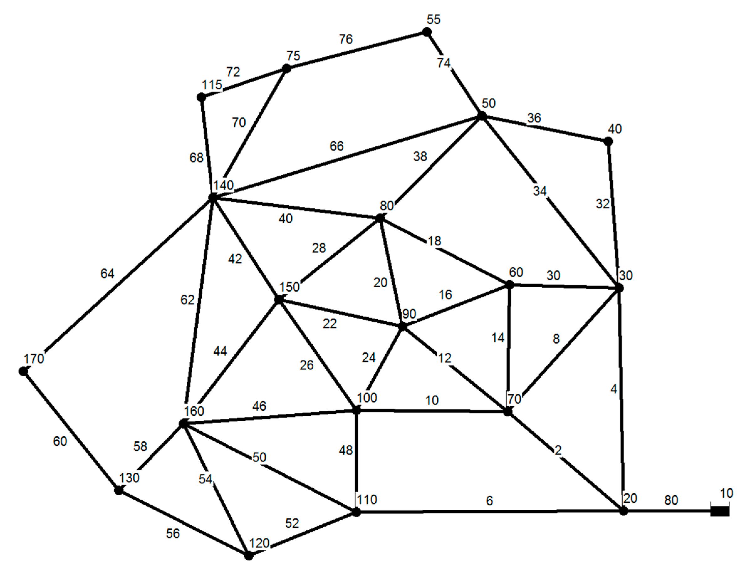
3.1. Applied Pipe Network
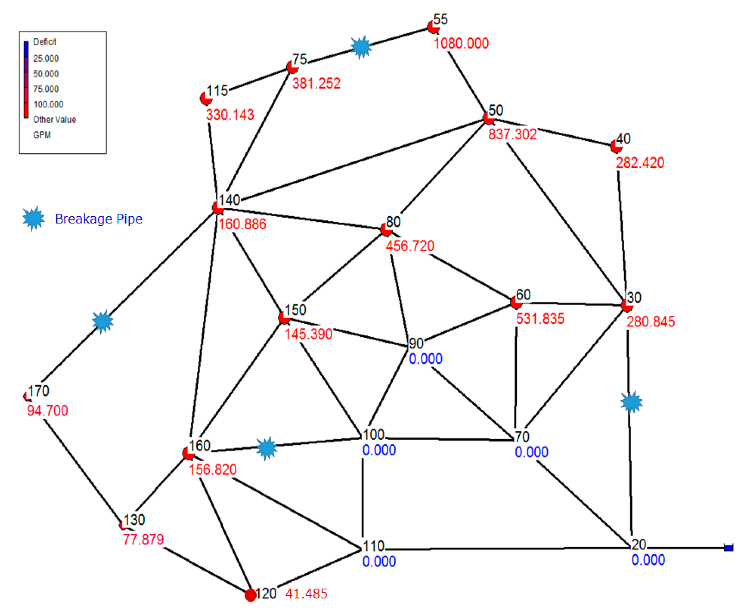
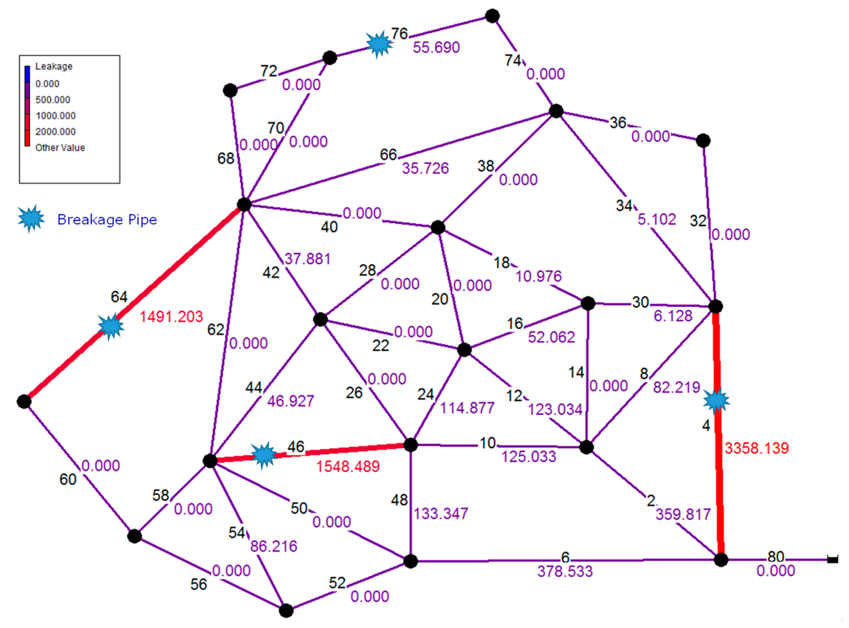
3.2. Earthquake Occurrence and Pipe Damage Scenario Setting
3.3. Application and Results
4. Conclusions
Author Contributions
Funding
Conflicts of Interest
References
- Whitman, R.V.; Hein, K.H. Damage Probability for a Water Distribution System. In Proceedings of the Current State of Knowledge of Lifeline Earthquake Engineering, New York, NY, USA, 30–31 August 1977; pp. 410–423. [Google Scholar]
- Hall, W.; Newmark, N. Seismic Design Criteria for Pipelines and Facilities. J. Tech. Councils ASCE 1978, 104, 91–107. [Google Scholar]
- Wang, Y. Seismic Performance Evaluation of Water Supply Systems. Ph.D. Thesis, Cornell University, Ithaca, NY, USA, January 2006. [Google Scholar]
- Shi, P. Seismic Response Modeling of Water Supply Systems. Ph.D. Thesis, Cornell University, Ithaca, NY, USA, January 2006. [Google Scholar]
- Shi, P.; O’Rourke, T.D.; Wang, Y. Simulation of earthquake water supply performance. In Proceedings of the 8th National Conference on Earthquake Engineering, Oakland, CA, USA, 18–22 April 1977; Paper No. 8NCEE-001295. EERI: Oakland, CA, USA. [Google Scholar]
- Wang, Y.; O’Rourke, T.D. Characterizations of seismic risk in Los Angeles water supply system. In Proceedings of the 5th China-Japan-US Symposium on Lifeline Earthquake Engineering, Haikou, China, 26–28 November 2007. [Google Scholar]
- Bonneau, A.L. Water Supply Performance during Earthquakes and Extreme Events. Ph.D. Thesis, Cornell University, Ithaca, NY, USA, 2008. [Google Scholar]
- Bonneau, A.L.; O’Rourke, T.D. Water Supply Performance during Earthquakes and Extreme Events; Technical Report MCEER-09-0003; University of Buffalo, State University of New York: Buffalo, NY, USA, 2009. [Google Scholar]
- Yoo, D.G. Seismic Reliability Assessment for Water Supply Networks. Ph.D. Dissertation, Korea University, Seoul, Korea, 2013. [Google Scholar]
- Hou, B.W.; Du, X.L. Comparative Study on Hydraulic Simulation of Earthquake-Damaged Water Distribution System. In Proceedings of the International Efforts in Lifeline Earthquake Engineering, Chengdu China, 2014; pp. 113–120. [Google Scholar]
- Yoo, D.G.; Jung, D.; Kang, D.; Kim, J.H.; Lansey, K. Seismic Hazard Assessment Model for Urban Water Supply Networks. J. Water Resour. Plan. Manag. ASCE 2016, 142. [Google Scholar] [CrossRef]
- Yoo, D.G.; Kang, D.; Kim, J.H. Optimal Design of Water Supply Networks for Enhancing Seismic Reliability. Reliab. Eng. Syst. Saf. 2016, 146, 79–88. [Google Scholar] [CrossRef]
- Rossman Lewis, A. EPANET 2: Users Manual; U.S. Environmental Protection Agency: Cincinnati, OH, USA, 2000.
- GIRAFFE. GIRAFFE User’s Manual; School of Civil and Environmental Engineering, Cornell University: Ithaca, NY, USA, 2008; Available online: https://www.cee.cornell.edu/cee (accessed on 14 February 2019).
- Ang, W.K.; Jowitt, P.W. Solution for Water Distribution Systems under Pressure-Deficient Conditions. J. Water Resour. Plan. Manag. 2006, 132, 175–182. [Google Scholar] [CrossRef]
- Giustolisi, O.; Savic, D.; Kapelan, Z. Pressure-Driven Demand and Leakage Simulation for Water Distribution Networks. J. Hydraul. Eng. 2008, 134, 626–635. [Google Scholar] [CrossRef]
- Baek, C.W. Development of HSPDA model for analysis of water distribution systems under abnormal operating conditions. Ph.D. Dissertation, Korea University, Seoul, Korea, 2007. [Google Scholar]
- Baek, C.W.; Jun, H.D.; Kim, J.H. Estimating the Reliability of Water Distribution Systems Using HSPDA Model and Distance Measure Method. J. Korea Water Resour. Assoc. 2010, 43, 769–780. [Google Scholar] [CrossRef]
- Baek, C.W.; Jun, H.D.; Kim, J.H. Estimation of the Reliability of Water Distribution Systems using HSPDA Model and ADF Index. J. Korea Water Resour. Assoc. 2010, 43, 201–210. [Google Scholar] [CrossRef]
- Giustolisi, O.; Kapelan, Z.; Savic, D.A. Extended Period Simulation Analysis Considering Valve Shutdowns. J. Water Resour. Plan. Manag. 2008, 134, 527–537. [Google Scholar] [CrossRef]
- Wu, Z.Y.; Wang, R.H.; Walski, T.M.; Yang, S.Y.; Bowdler, D.; Baggett, C.C. Extended Global—gradient Algorithm for Pressure-dependent Water Distribution Analysis. J. Water Resour. Plan. Manag. 2009, 135, 13–22. [Google Scholar] [CrossRef]
- Lee, H.M.; Yoo, D.G.; Kang, D.; Jun, H.; Kim, J.H. Uncertainty quantification of pressure-driven analysis for water distribution network modeling. Water Sci. Technol. Water Suppl. 2016, 16, 599–610. [Google Scholar] [CrossRef]
- May, J. Leakage, pressure and control. In Proceedings of the BICS International Conference on Leakage Control, London, UK, March 1994. [Google Scholar]
- Klise, K.A.; Bynum, M.; Moriarty, D.; Murray, R. A software framework for assessing the resilience of drinking water systems to disasters with an example earthquake case study. Environ. Model. Softw. 2017, 95, 420–431. [Google Scholar] [CrossRef] [PubMed]
- Yoo, D.G.; Shin, E.H. Recent Trends and Proper Applications of Hydraulic Analysis Technique of Water Distribution Networks. Mag. Korean Soc. Hazard Mitig. 2018, 18, 45–51. [Google Scholar]
- Puchovsky, M.T. Automatic sprinkler systems handbooks; National Fire Protection Association (NFPA): Quincy, MA, USA, 1999. [Google Scholar]
- Gupta, R.; Bhave, P.R. Comparison of methods for predicting deficient-network performance. J. Water Resour. Plan. Manag. 1996, 122, 214–217. [Google Scholar] [CrossRef]
- Tanyimboh, T.T.; Tabesh, M. Discussion comparison of methods for predicting deficient-network performance. J. Water Resour. Plan. Manag. 1997, 123, 369–370. [Google Scholar] [CrossRef]
- Mays, L. Water Supply Systems Security; McGraw-Hill Education: New York, NY, USA, 2004. [Google Scholar]
- Wagner, J.M.; Shamir, U.; Marks, D.H. Water distribution reliability: Simulation methods. J. Water Resour. Plan. Manag. 1988, 114, 276–294. [Google Scholar] [CrossRef]
- Lambert, A. What do we know about pressure: Leakage relationships in distribution systems? In Proceedings of the IWA Conference in Systems Approach to Leakage Control and Water Distribution System Management, International Water Association, Brno, Czech Republic, 16–18 May 2001. [Google Scholar]
- Lambert, A.; Fantozzi, M.; Shepherd, M. Pressure: Leak flow rates using FAVAD: An improved fast-track practitioner’s approach. In Proceedings of the Computing and Control for the Water Industry (CCWI 2017), Sheffield, UK, 5–7 September 2017. [Google Scholar]
- Gupta, R.; Bhave, P.R. Reliability analysis of water-distribution systems. J. Environ. Eng. 1994, 120, 447–461. [Google Scholar] [CrossRef]
- Cullinane, M.; Lansey, K.; Mays, L. Optimization-availability-based design of water-distribution networks. J. Hydraul. Eng. 1991, 118, 420–441. [Google Scholar] [CrossRef]
- Tabucchi, T.; Davidson, R.; Brink, S. Simulation of post-earthquake water supply system restoration. Civil Eng. Environ. Syst. 2010, 27, 263–279. [Google Scholar] [CrossRef]
- Lansey, K. Sustainable, robust, resilient, water distribution systems. In Proceedings of the 14th Water Distribution Systems Analysis Conference, Adelaide, Australia, 24–27 September 2012; pp. 1–18. [Google Scholar]
- Walski, T.; Brill, E.; Gessler, J., Jr.; Goulter, I.; Jeppson, R.; Lansey, K.; Lee, H.; Liebman, J.; Mays, L.; Morgan, D.; et al. Battle of the Network Models: Epilogue. J. Water Resour. Plan. Manag. 1987, 113, 191–203. [Google Scholar] [CrossRef]
- Jung, D.; Kang, D.; Kim, J.H.; Lansey, K. Robustness-based design of water distribution systems. J. Water Resour. Plan. Manag. 2014, 140, 04014033. [Google Scholar] [CrossRef]
- Yoo, D.G.; Jung, D.; Kang, D.; Kim, J.H. Seismic-reliability-based optimal layout of a water distribution network. Water 2016, 8, 50. [Google Scholar] [CrossRef]
- Lee, H.M.; Yoo, D.G.; Kim, J.H.; Kang, D. Hydraulic simulation techniques for water distribution networks to treat pressure deficient conditions. J. Water Resour. Plan. Manag. 2015, 142, 06015003. [Google Scholar] [CrossRef]


| Simulation Situation | Water Usage Relationship | Example |
|---|---|---|
| Normal situation | Supply = total usage(demand) | New planning and design of mid-long term WSNs |
| Supply = usage + leakage quantity | Analysis of the current pipe network considering general leakage quantity | |
| Abnormal situation | Supply = usage + leakage quantity | Analysis of the pipe network in situations where the effect of leakage quantity is dominant |
| Supply < usage | When the supply is insufficient due to drought, changes in demand, etc. | |
| Supply < usage + leakage quantity | When pipe breakage has occurred due to various causes |
| Purpose of Pipe Network Analysis | Description | Results of Demand DrivenAnalysis | Appropriate Method | Related Research |
|---|---|---|---|---|
| Emergency linkage between water supply areas | When a problem has occurred in the block, figure out the quantity of water that can supplied in an emergency and the areas whether the water can be supplied following the opening of emergency linkage pipelines | The sufficient head is satisfied | DDA | Secure local waterworks supply stability |
| Poor outflow (the sufficient head has not been reached) | PDD | |||
| Not suppliable (negative pressure occurred) | PDD | |||
| Hydraulic review following pipe doubling | Figure out the suppliable areas in cases where water is supplied through doubled pipes as problems occurred in large caliber pipes | The sufficient head is satisfied | DDA | Secure wide regional waterworks supply stability |
| Poor outflow (the sufficient head has not been reached) | PDD | |||
| Not suppliable (negative pressure occurred) | PDD | |||
| Supply shortage simulation | Hydraulic review in cases where the block inflow rate (supply) is smaller than the usage | Not suppliable areas/poor outflow areas appeared | PDDs | Local project in which restrictive water rationing is usual |
| Simulation of changes in leakage quantities between before and pipe network maintenance | Hydraulic analysis before and after pipe network maintenance considering leakage quantities, usage, etc. | Analysis of areas where water flow rates are high | DDA | Pipe network maintenance master plan |
| Cases where the ratio of the leakage quantity to the usage is high because the water flow rate is high | PDL | |||
| Analysis of pipe network breakage due to accidents or disasters | Analysis of pipe breakage due to accidents or cases where many pipes or facilities such as water distribution reservoirs have been broken | When the effect of single pipe breakage is small | DDA | Establish emergency response plans |
| When the effect of single pipe breakage is large | PDDL | |||
| When the effect of breakage of many pipes or water distribution reservoirs due to large scaled earthquakes is large | PDDL |
| Status of Pipe | REVAS.NET | Proposed Model |
|---|---|---|
| Leakage | The emitter coefficient is entered into the bottom node of the pipe where the leakage has occurred (single coefficient) | The C1 and C2 values of the FAVAD equation are entered into the pipe where the leakage has occurred (leakage coefficient/breakage coefficient) |
| Breakage | (1) During the simulation of hydraulic analysis, the pipe state is set to “closed” to block flows (2) The emitter coefficient is entered into the top node of the broken pipe | (1) During the simulation of hydraulic analysis, the pipe state is set to “closed” to block flows (2) The FAVAD coefficient is entered into the broken pipe |
| Hydraulic Simulation Technique | Quasi-PDA | Full-PDA |
| Scenario | Number of Pipe | ||
|---|---|---|---|
| Normal | Leak | Breakage | |
| S1 | 18 | 16 | 4 |
| S3 | 16 | 19 | 3 |
| S4 | 16 | 19 | 3 |
| S7 | 18 | 17 | 3 |
| S8 | 22 | 15 | 1 |
| S10 | 10 | 27 | 1 |
| S11 | 10 | 24 | 4 |
| S12 | 16 | 19 | 3 |
| S13 | 22 | 11 | 5 |
| S14 | 17 | 18 | 3 |
| S15 | 18 | 16 | 4 |
| S17 | 9 | 28 | 1 |
| S18 | 10 | 23 | 5 |
| S22 | 6 | 29 | 3 |
| S23 | 15 | 19 | 4 |
| S24 | 22 | 14 | 2 |
| S25 | 15 | 21 | 2 |
| S26 | 14 | 21 | 3 |
| S27 | 23 | 11 | 4 |
| S28 | 19 | 18 | 1 |
| Average | 15.80 | 19.25 | 2.95 |
| Scenario | Proposed Model | REVAS.NET | |||||
|---|---|---|---|---|---|---|---|
| Actual Water Supply (LPS) | Deficit (LPS) | Outflow (LPS) | Leakage (LPS) | Ss | Lri | Ss | |
| S1 | 806 | 306 | 1314 | 508 | 0.725 | 0.456 | 0.202 |
| S3 | 1010 | 103 | 1369 | 360 | 0.907 | 0.323 | 0.354 |
| S4 | 1048 | 65 | 1530 | 482 | 0.942 | 0.433 | 0.246 |
| S7 | 819 | 293 | 1246 | 427 | 0.736 | 0.384 | 0.199 |
| S8 | 724 | 389 | 1080 | 356 | 0.651 | 0.320 | 0.305 |
| S10 | 1074 | 39 | 1343 | 269 | 0.965 | 0.242 | 0.459 |
| S11 | 1028 | 84 | 1566 | 538 | 0.924 | 0.483 | 0.225 |
| S12 | 1060 | 53 | 1424 | 364 | 0.953 | 0.327 | 0.576 |
| S13 | 696 | 417 | 1095 | 399 | 0.625 | 0.359 | 0.348 |
| S14 | 956 | 157 | 1365 | 409 | 0.859 | 0.367 | 0.149 |
| S15 | 995 | 117 | 1395 | 400 | 0.894 | 0.359 | 0.383 |
| S17 | 1070 | 43 | 1380 | 310 | 0.962 | 0.279 | 0.490 |
| S18 | 954 | 158 | 1416 | 461 | 0.858 | 0.415 | 0.264 |
| S22 | 1062 | 51 | 1703 | 641 | 0.954 | 0.576 | 0.261 |
| S23 | 937 | 176 | 1457 | 520 | 0.842 | 0.467 | 0.356 |
| S24 | 1073 | 40 | 1346 | 273 | 0.964 | 0.246 | 0.416 |
| S25 | 1059 | 54 | 1441 | 382 | 0.951 | 0.343 | 0.457 |
| S26 | 1042 | 71 | 1383 | 342 | 0.936 | 0.307 | 0.370 |
| S27 | 881 | 232 | 1366 | 485 | 0.792 | 0.436 | 0.300 |
| S28 | 1081 | 32 | 1277 | 197 | 0.971 | 0.177 | 0.582 |
| Average | 969 | 144 | 1375 | 406 | 0.871 | 0.365 | 0.347 |
| Number of Leaked Pipe | Proposed Model | REVAS.NET | |
|---|---|---|---|
| Ss | Lri | Ss | |
| 11 | 0.708 | 0.397 | 0.324 |
| 14 | 0.964 | 0.246 | 0.416 |
| 15 | 0.651 | 0.320 | 0.305 |
| 16 | 0.085 | 0.049 | 0.090 |
| 17 | 0.736 | 0.384 | 0.199 |
| 18 | 0.915 | 0.272 | 0.365 |
| 19 | 0.934 | 0.361 | 0.392 |
| 21 | 0.944 | 0.325 | 0.414 |
| 23 | 0.858 | 0.415 | 0.264 |
| 24 | 0.924 | 0.483 | 0.225 |
| 27 | 0.965 | 0.242 | 0.459 |
| 28 | 0.962 | 0.279 | 0.490 |
| 29 | 0.954 | 0.576 | 0.261 |
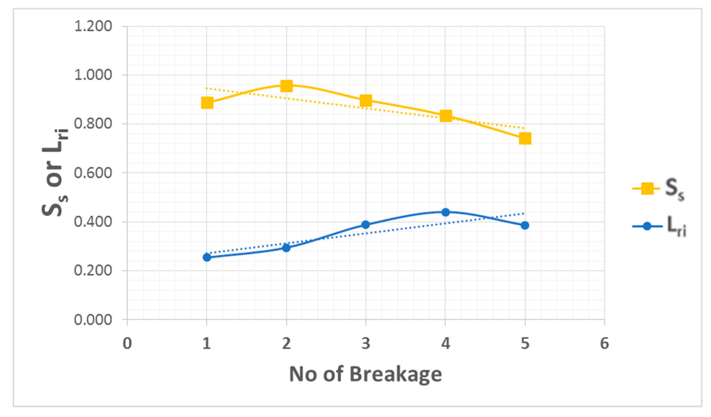
| Number of Break Pipe | Proposed Model | REVAS.NET | |
|---|---|---|---|
| Ss | Lri | Ss | |
| 1 | 0.887 | 0.254 | 0.459 |
| 2 | 0.958 | 0.294 | 0.437 |
| 3 | 0.898 | 0.388 | 0.308 |
| 4 | 0.835 | 0.440 | 0.293 |
| 5 | 0.741 | 0.387 | 0.306 |
© 2019 by the authors. Licensee MDPI, Basel, Switzerland. This article is an open access article distributed under the terms and conditions of the Creative Commons Attribution (CC BY) license (http://creativecommons.org/licenses/by/4.0/).
Share and Cite
Yoo, D.G.; Lee, J.H.; Lee, B.Y. Comparative Study of Hydraulic Simulation Techniques for Water Supply Networks under Earthquake Hazard. Water 2019, 11, 333. https://doi.org/10.3390/w11020333
Yoo DG, Lee JH, Lee BY. Comparative Study of Hydraulic Simulation Techniques for Water Supply Networks under Earthquake Hazard. Water. 2019; 11(2):333. https://doi.org/10.3390/w11020333
Chicago/Turabian StyleYoo, Do Guen, Joo Ha Lee, and Bo Yeon Lee. 2019. "Comparative Study of Hydraulic Simulation Techniques for Water Supply Networks under Earthquake Hazard" Water 11, no. 2: 333. https://doi.org/10.3390/w11020333
APA StyleYoo, D. G., Lee, J. H., & Lee, B. Y. (2019). Comparative Study of Hydraulic Simulation Techniques for Water Supply Networks under Earthquake Hazard. Water, 11(2), 333. https://doi.org/10.3390/w11020333