Hydrological Model Supported by a Step-Wise Calibration against Sub-Flows and Validation of Extreme Flow Events


Abstract
1. Introduction
2. Materials and Methods
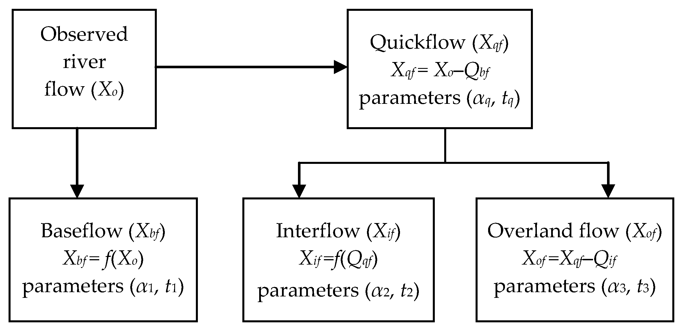
2.1. Separation of Sub-Flows
- (a)
- select a time scale t1 which denotes the baseflow filtering constant such that w = 0.5 × (1 + t1) and w = 0.5 × t1 in the cases when t1 is odd and even, respectively,
- (b)
- if Xo comprises a subset xo from the pth to the uth value of Xo, obtain the filter term b using:where hj is the size of the sub-sample in the jth time slice (i.e., xo from the pth to the uth data value), α1 denotes the baseflow coefficient, and the terms p and u can be varied for j = 1, 2, ..., n as follows:It is vital to note that the application of Equations (1) and (2) is done in a step-wise way. For instance, if t1 = 10, it means w = 5. Now, we have to vary j from 1 to n, and let us assume that n = 100. Each time a new j is being considered, the terms p and u of Equation (1) are determined based on the three conditions given in Equation (2). Using t1 = 10, w = 5, and n = 100, below is an illustration of how the terms p and u can be determined for every new value of j which is varied by setting j = 1, 2, ..., 100.
- (i)
- If j = 1, it means j < w and thus, using the first conditional part of Equation (2), p = 1, and u = 10 + 1 – 5 – 1 = 5. This means that for j = 1, the summation of the flow xo according to Equation (1) is done from the 1st to the 5th value.
- (ii)
- If j = 15, it means j > w and thus, using the second conditional component of Equation (2), p = 15 – 5 + 1 = 11, and u = 15 + 5 = 20. This means that for j = 15, the summation of the flow xo based on Equation (1) is done from the 11th to the 20th value.
- (iii)
- If j = 96, it means j > (n − w) and j ≤ n; therefore, using the third conditional part of Equation (2), p = 96 – 5 + 1 = 92, and u = 100. This means that for j = 96, the summation of the flow xo according to Equation (1) is done from the 92nd to the 100th value.
- (c)
- for j = 1, 2, ..., n, at the time step j, if b(j) < xo(j), xbf (j) = b(j), otherwise, xbf (j) = xo(j), and the quick flow component (Xqf) of Xo can be given by xqf (j) = xo(j) − xbf (j).
- (a)
- select the time scale t2 which denotes the interflow filtering constant and let w = 0.5 × (1 + t2) and w = 0.5 × t2 in the cases when t2 is odd and even, respectively,
- (b)
- compute the interflow component c using:where α2 denotes the interflow coefficient, h(j) is the sub-sample size in the jth time slice (i.e., Xqf from the pth to the uth data point), and for j = 1, 2, ..., n, the terms p and u can be varied as in Equation (2). The application of Equation (3) is in a similar way as described for Equation (1).
- (c)
- for j = 1, 2, ..., n, if c(j) < xqf (j), xif (j) = c(j), otherwise, xif (j) = xqf (j), and the overland flow component (Xof) of Xo at the time step j can be given by xof (j) = xqf (j) − xif (j).
2.2. Rainfall-Runoff Modeling
2.2.1. HMSV Structure Identification
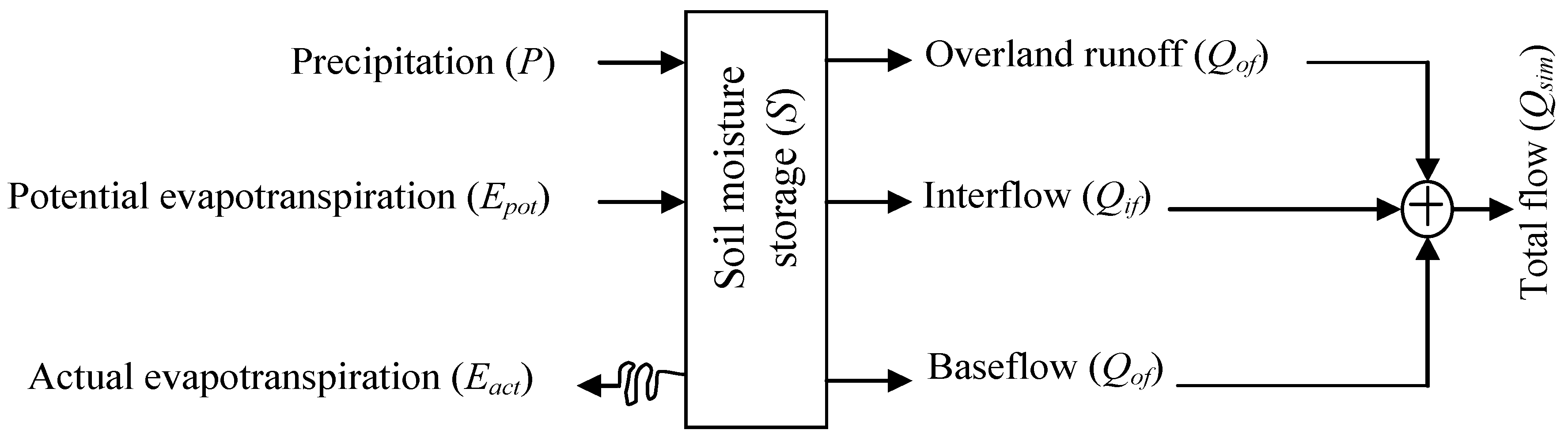
Soil Moisture Storage
Evapotranspiration
Runoff
- (1)
- To compute Qbf, select baseflow recession constant ta. Apply Equation (1) to soil moisture (S) instead of xo while replacing t1 with ta in Equations (1) and (2) to obtain instead of b.
- (2)
- To compute Qif, chose interflow recession constant tb. Apply Equation (1) to S instead of xo while replacing t1 with tb in Equations (1) and (2) to obtain in the place of b.
- (3)
- For Qof, chose constants tu and tv. By applying Equation (1) to S, replace t1 with tu in Equations (1) and (2) to obtain instead of b. Finally to the series N of Equation (7), apply Equation (1) while replacing t1 with tv in Equations (1) and (2) to obtain in the place of b.
Initial Conditions
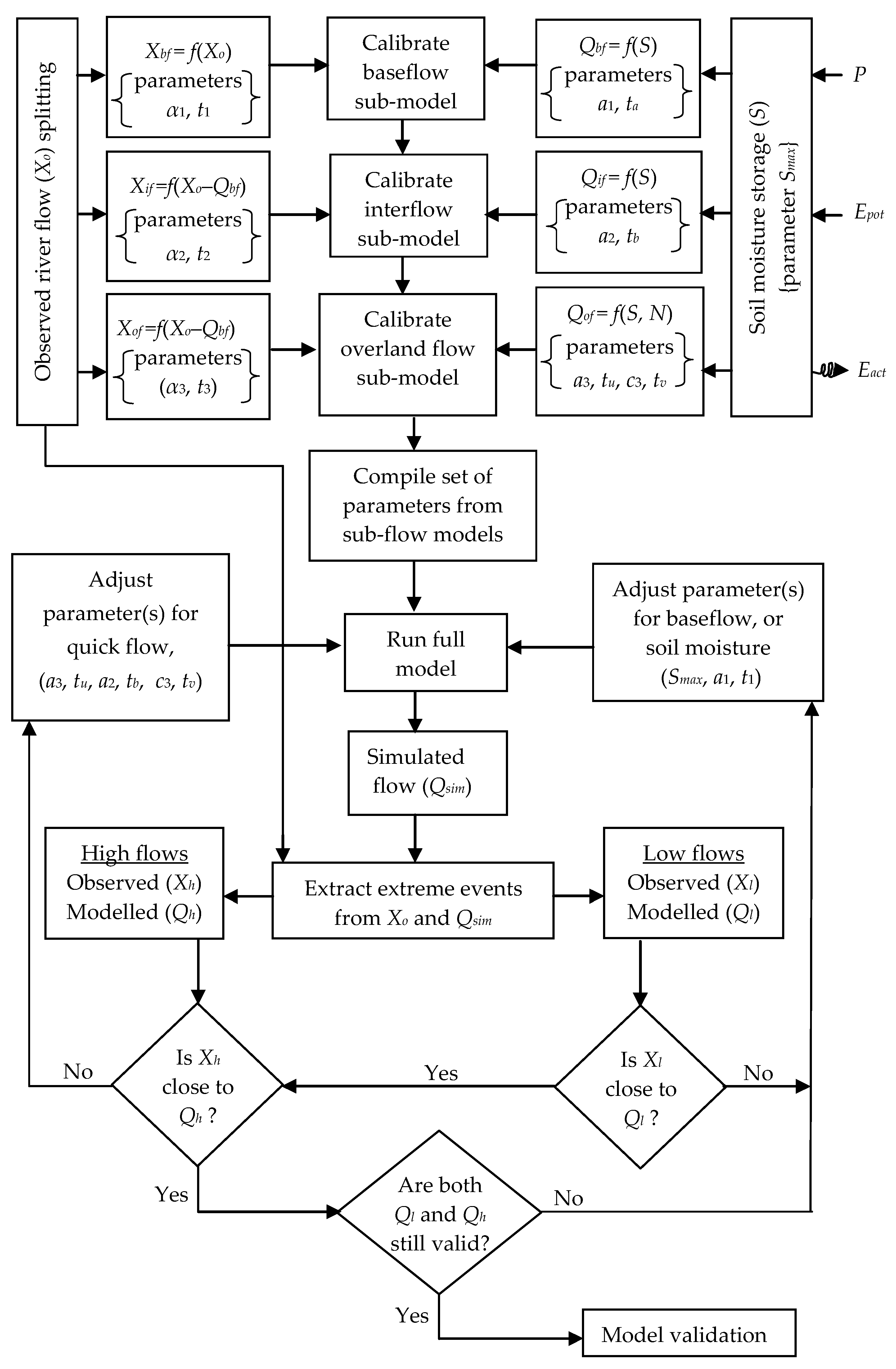
2.2.2. HMSV Calibration Framework
- (1)
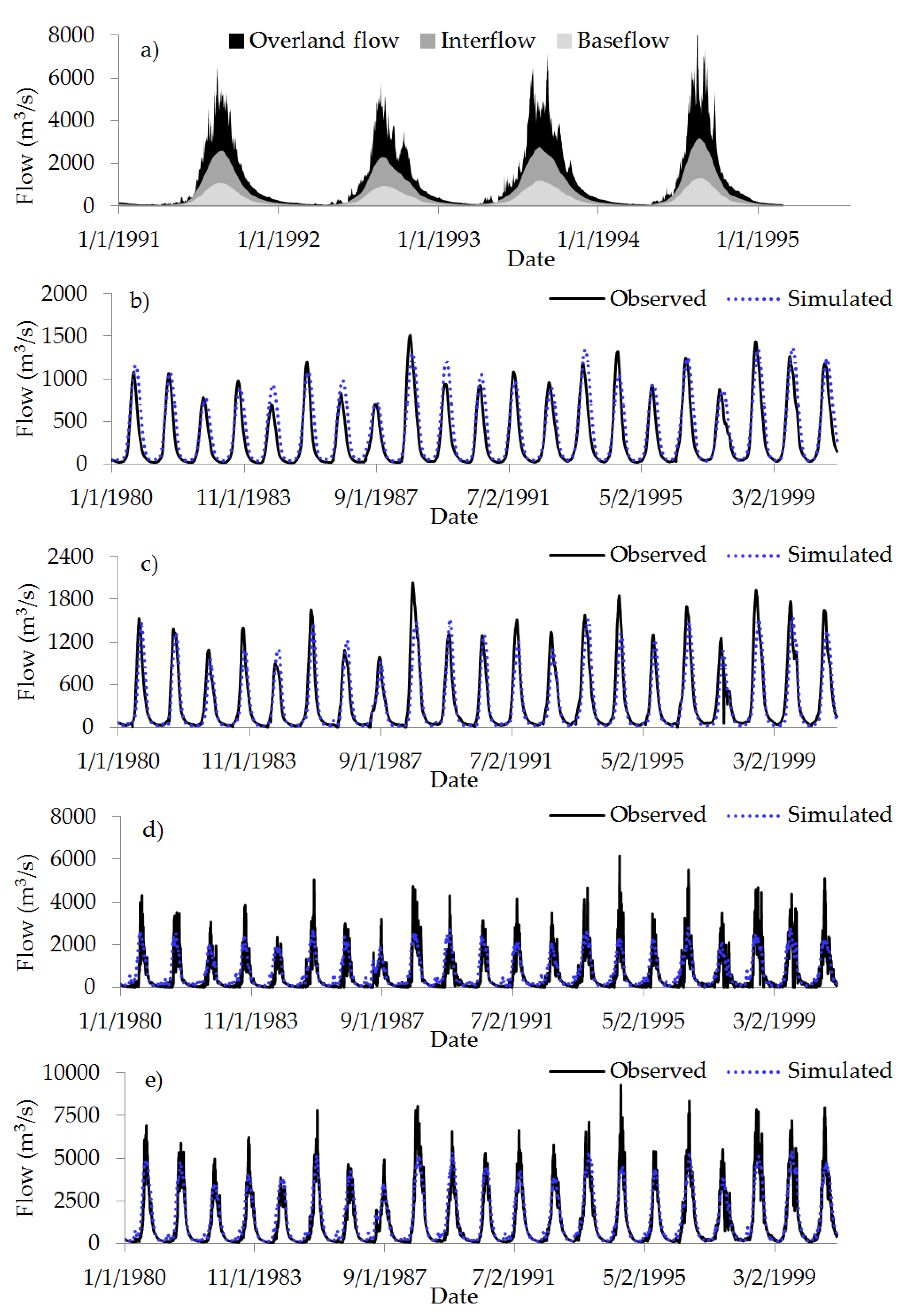
- the observed flow (Xo) is separated into various sub-flows including baseflow (Xbf), interflow (Xif), and overland flow (Xof),
- (2)
- using the baseflow sub-model, the modeled baseflow (Qbf) is calibrated against Xbf,
- (3)
- using the interflow sub-model, the modeled interflow (Qif) is calibrated against Xif,
- (4)
- using the overland sub-model, the modeled overland flow (Qof) is calibrated against Xof,
- (5)
- the parameters from the various sub-flow models are combined and used to run the full model from which total simulated flow (Qsim) is obtained.
- (i)
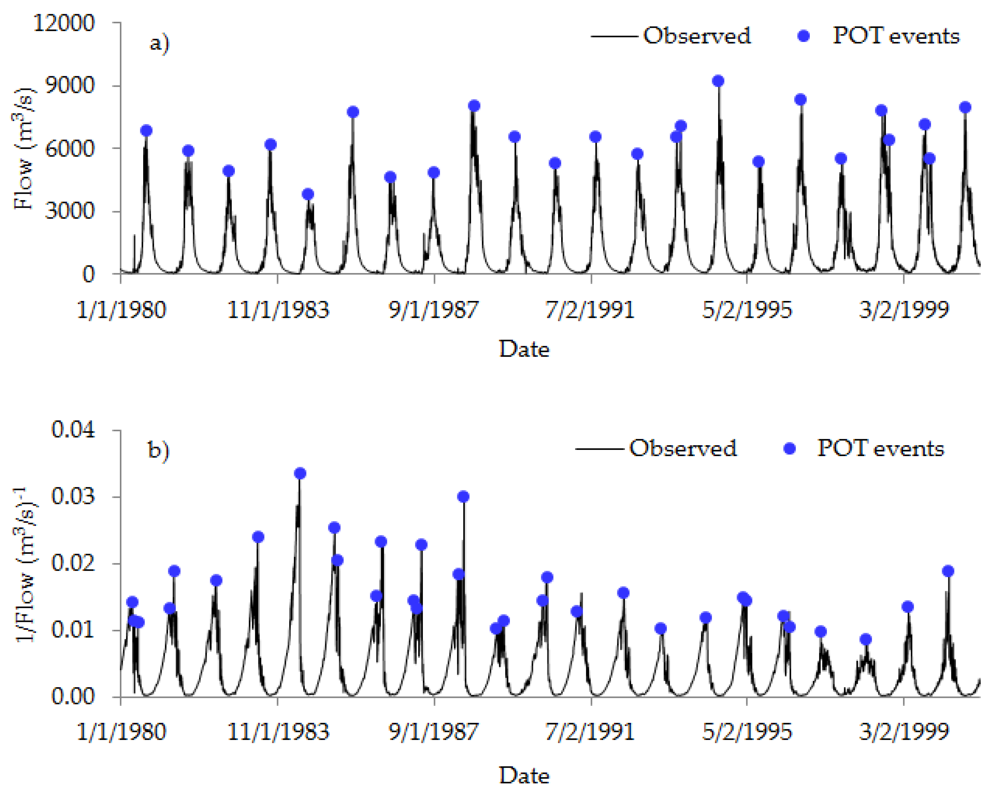
- Hydrological extremes are extracted from both observed river flow (Xo) and simulated flow (Xsim). Here, the Peak Over Threshold (POT) approach can be adopted for extraction of the hydrological extremes (see Appendix A for details). It is important to note that the POT events from both Xo and Xsim should also be extracted using the same set of parameters stipulated to define the independency criteria. If the data for calibration is long enough (say 30 years or more), annual maxima and minima series could also be used for the checking the validity of the hydrological extremes.
- (ii)
- If the observed (Xl) and modeled (Ql) low flow quantiles are not comparable, parameter(s) which control baseflow generation can be adjusted to obtain new simulated flow. If Xl and Ql are comparable, focus is thereafter turned to high flows according to step (iii).
- (iii)
- To minimize the mismatch between the observed (Xh) and modeled (Qh) high flow quantiles, parameter(s) which control soil moisture and quick flow (interflow and overland flow) runoff generation can be adjusted, and when the full model is run, new simulated flow series is obtained.
- (iv)
- It is possible that Step (iii) can lead to some increase in the mismatch between the observed (Xl) and modeled (Ql) low flow quantiles based on Step (ii). Therefore, at this point, again, it is important to check on the validity of both high flows and low flows and some parameters may also be changed if need be.
- (v)
- The final simulated series is the model-based flow which reasonably reproduces both high and low flow quantiles.
2.3. Case Study
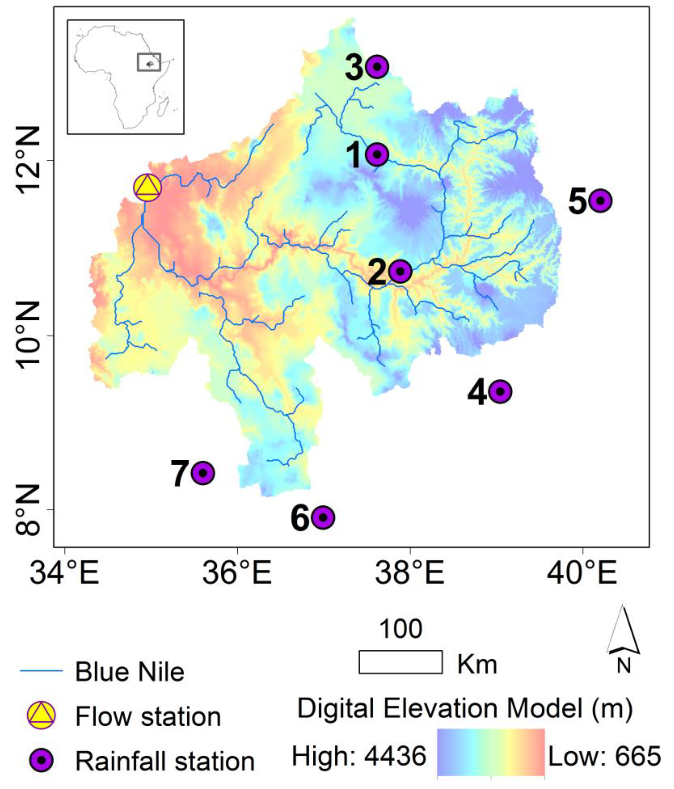
2.3.1. Data and Study Area
2.3.2. Rainfall-Runoff Modeling
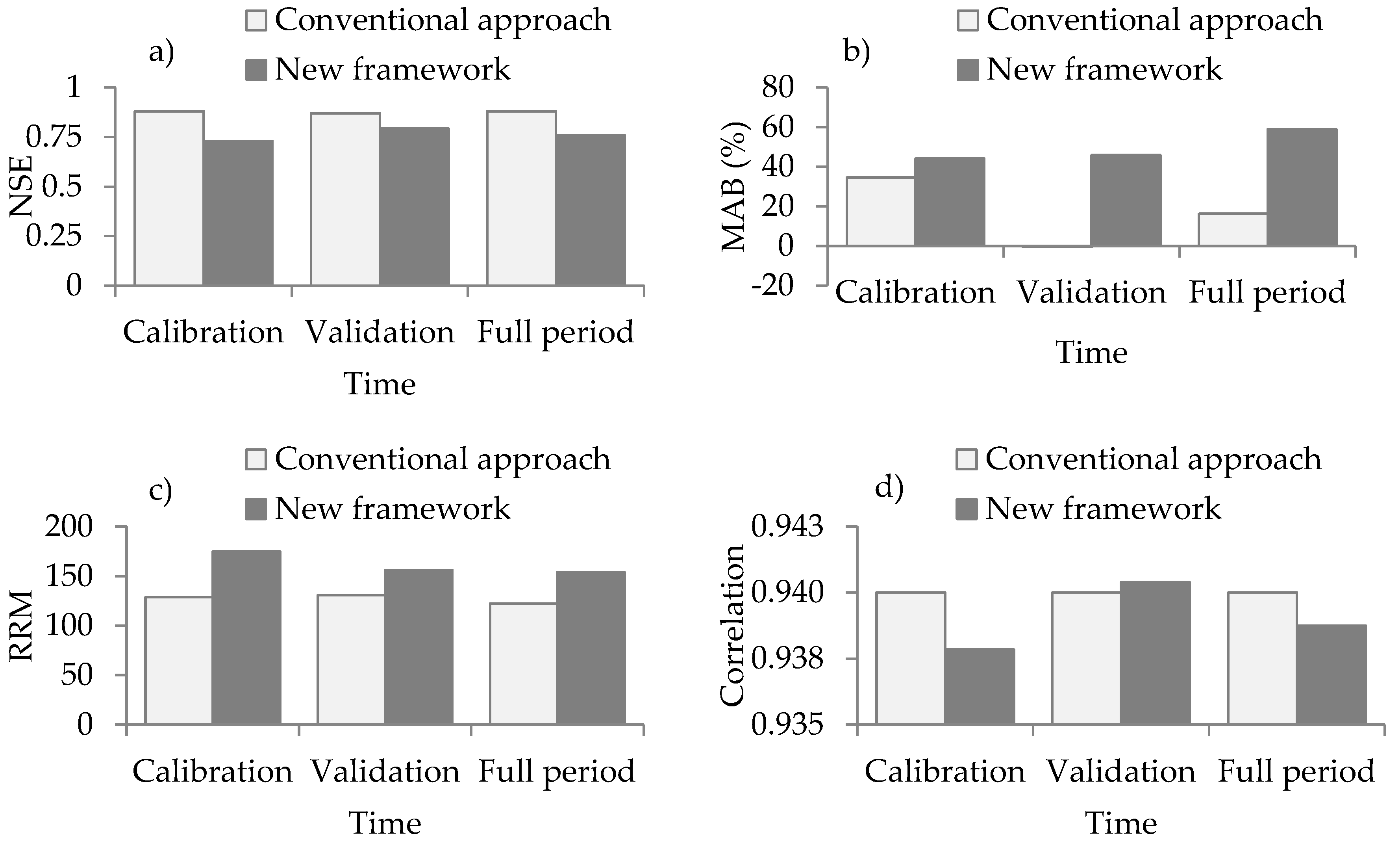
2.3.3. Comparison of Conventional Approach and New Framework for Calibration
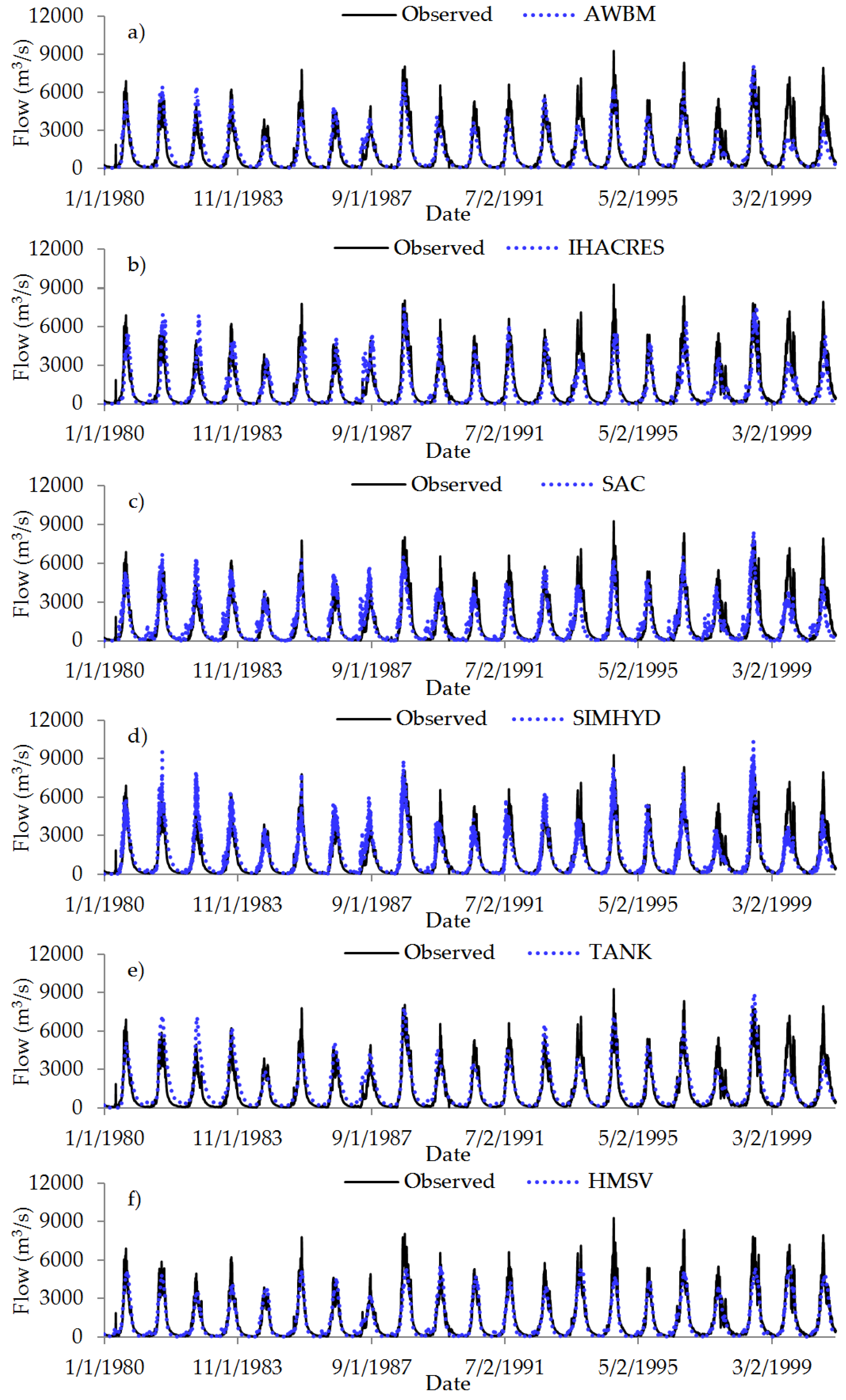
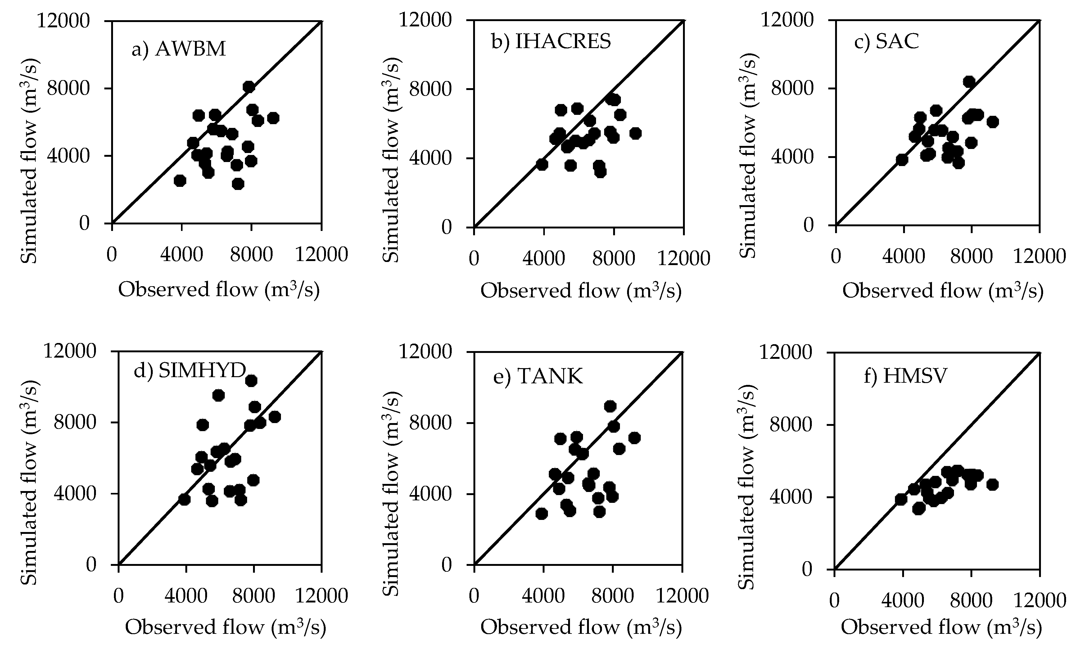
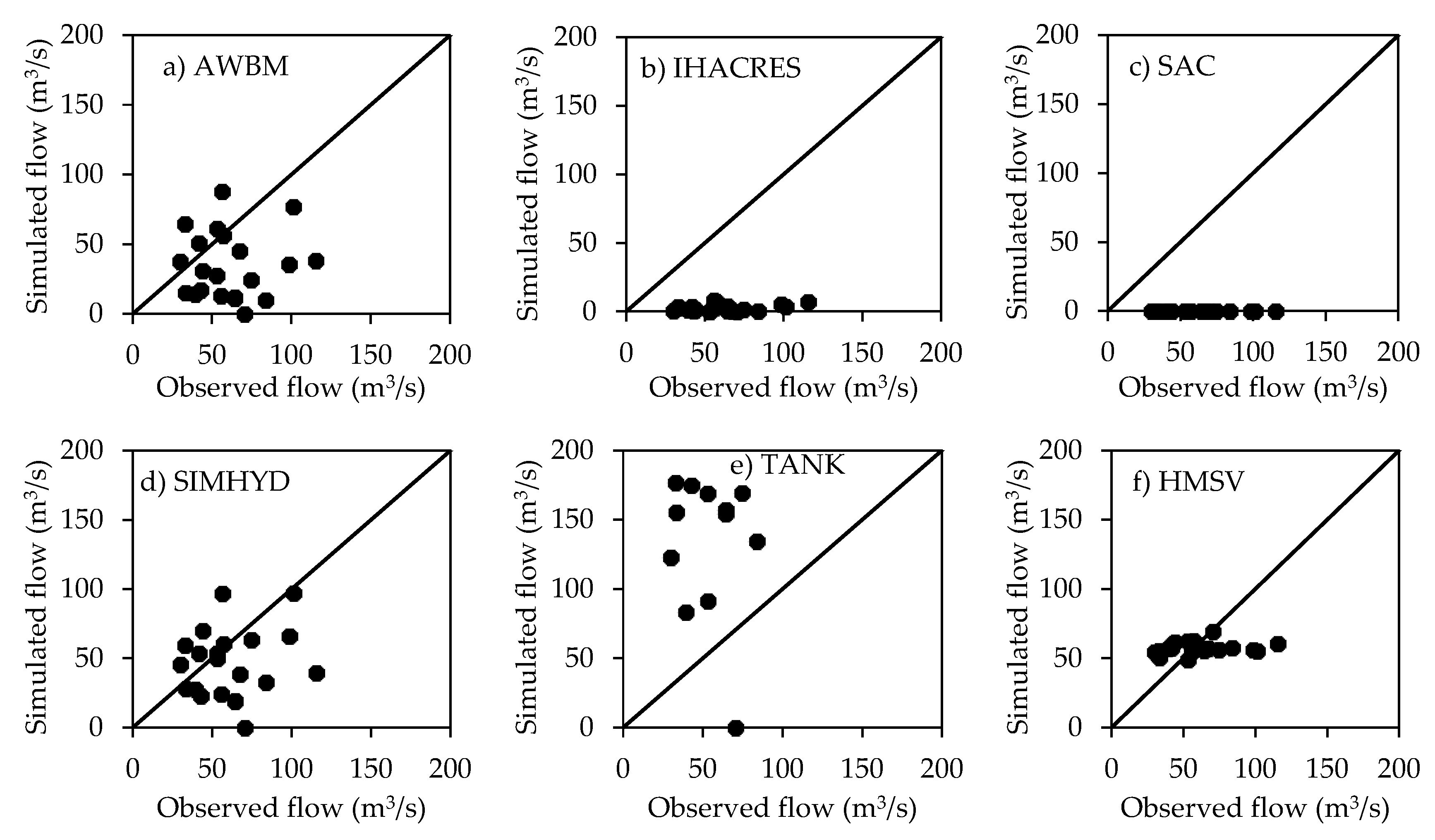
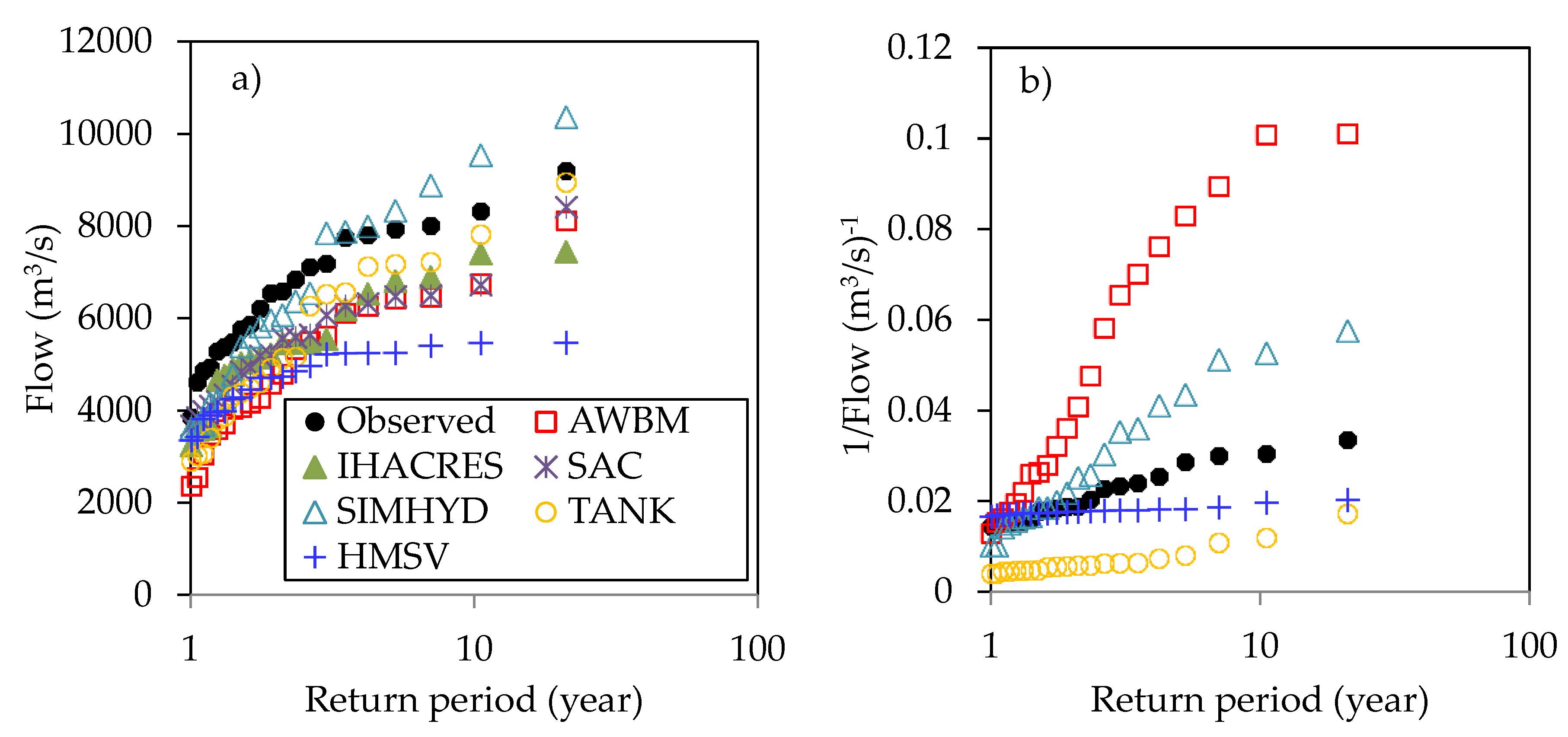
2.3.4. Comparison of HMSV and Conventional Models
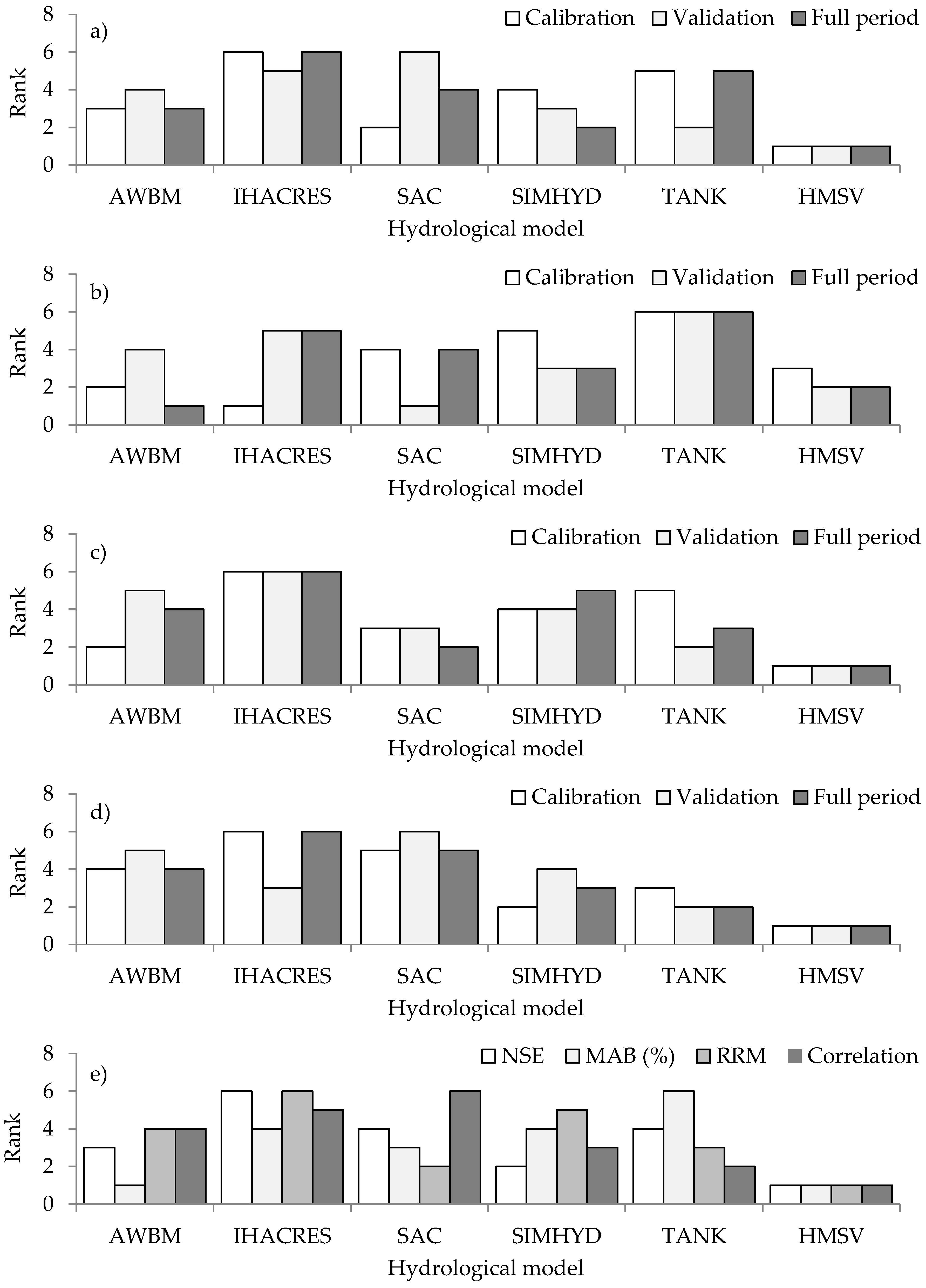
- (i)
- models were ranked from 1 to 6 based on the NSE values. The ranking was done such that ranks 1 and 6 were for the best and worst models, respectively. This procedure was done separately for calibration and validation periods as well as considering the full data period.
- (ii)
- just like in (i), the models were ranked based on MAB. The model with the lowest (highest) MAB was given rank 1 (6) denoting the best (worst) model. Again, this procedure was separately done for calibration and validation periods as well as the full data period.
- (iii)
- step (ii) was repeated using the RRM instead of MAB, and
- (iv)
- step (i) was repeated using the correlation instead of NSE,
- (v)
- the sum of ranks from calibration and validation periods as well as the full data period was obtained for NSE, MAB, RRM, and correlation, of steps (i) to (iv), respectively, and
- (vi)
- Finally, the best (worst) model was taken as that with the smallest (largest) sum of ranks.
3. Results and Discussion
3.1. Discharge Splitting and Modeling of Sub-Flows
3.2. Comparison of HMSV and Conventional Models
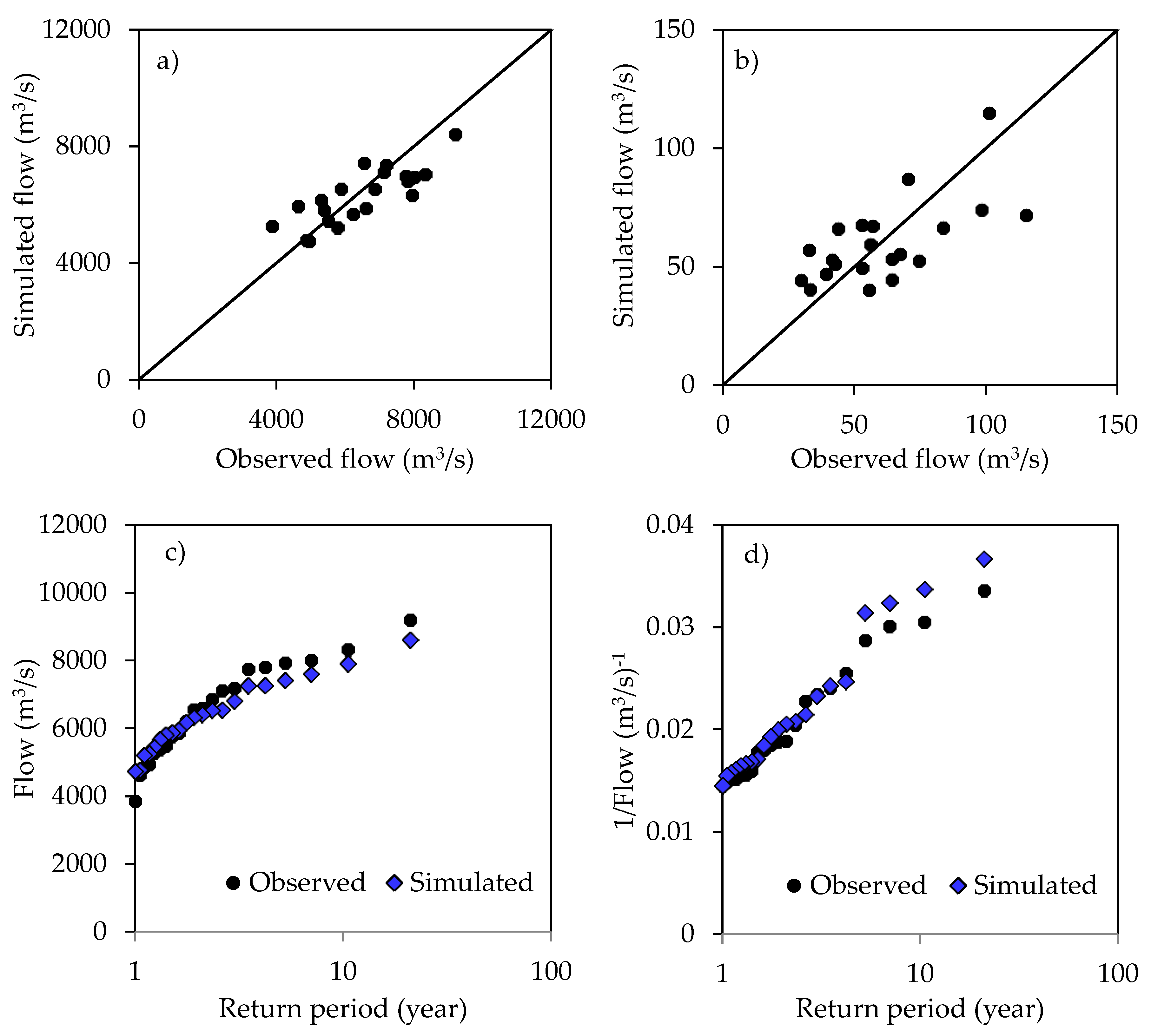
3.3. New Framework versus the Conventional Approach
4. Conclusions
Funding
Acknowledgments
Conflicts of Interest
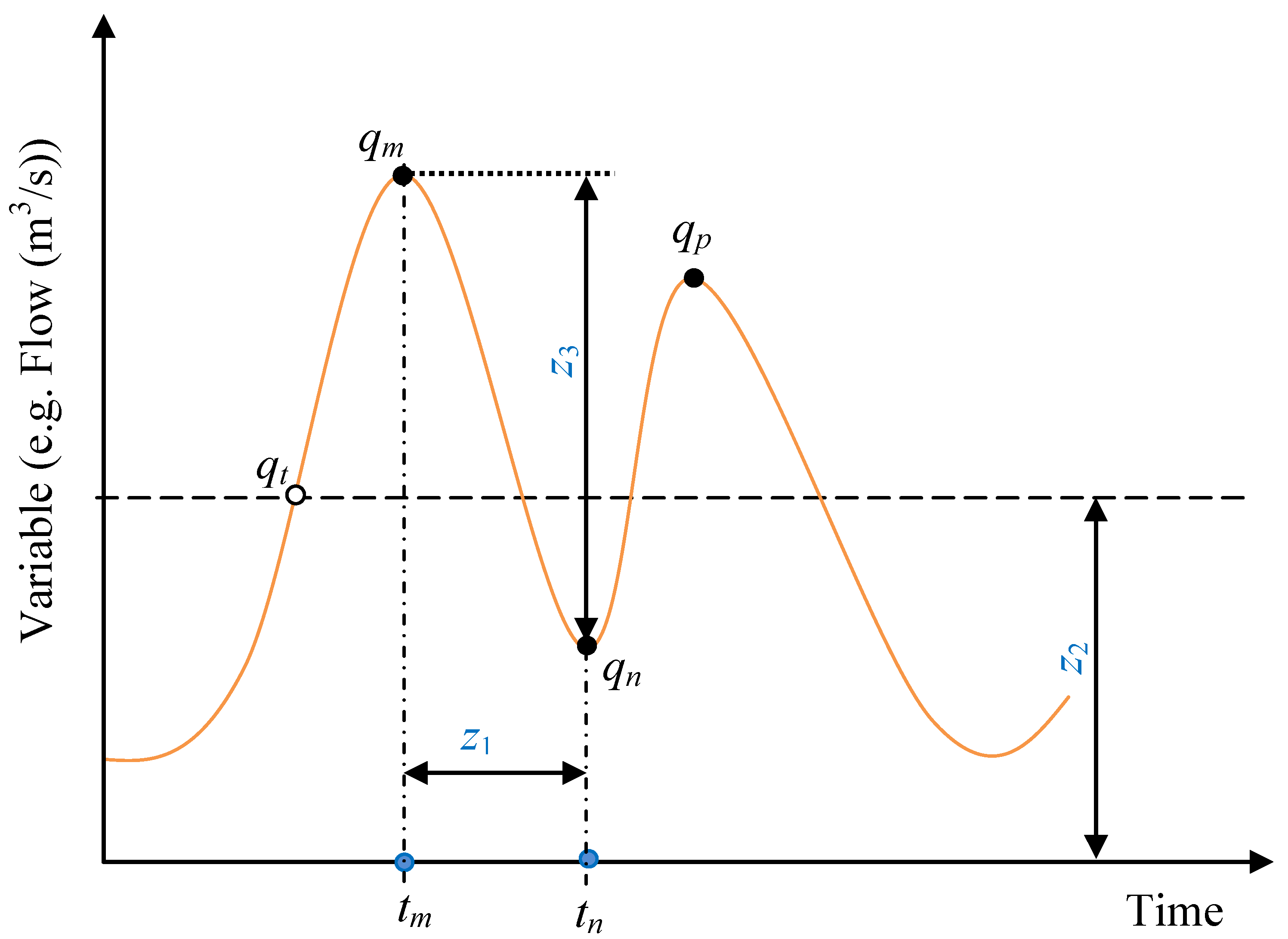
Appendix A Further Information on the Extraction of Hydrological Extremes
- (i)
- z1 or (tn – tm) is not less than the stipulated inter-event time τ,
- (ii)
- z3 or (qm – qn) divided by qm and multiplied by 100 is greater than the independency ratio γ stipulated in percentage,
- (iii)
- the event qm is greater than the threshold qt or z2. For a more stringent threshold than using qm > qt, we can consider qn < qt < qm.


Appendix B List of Optimal Model Parameters after Calibration

| SNo. | Parameter | Unit | Value |
|---|---|---|---|
| SACRAMENTO | |||
| 1 | Additional fraction of pervious area (Adimp) | (-) | 0.0025 |
| 2 | Lower Zone Free Water Primary Maximum (Lzfpm) | (mm) | 49.1030 |
| 3 | Lower Zone Free Water Supplemental Maximum (Lzfsm) | (m) | 49.5920 |
| 4 | Ratio of water in LZFPM (Lzpk) | (mm) | 0.0079 |
| 5 | Ratio of water in LZFSM (Lzsk) | (mm) | 0.0503 |
| 6 | Lower Zone Tension Water Maximum (Lztwm) | (mm) | 224.410 |
| 7 | Impervious fraction of the basin (Pctim) | (-) | 0.0201 |
| 8 | Minimum proportion of percolation (Pfree) | (-) | 0.9965 |
| 9 | Exponential percolation rate (Rexp) | (-) | 0.0329 |
| 10 | Fraction of water unavailable for transpiration (Rserv) | (-) | 0.3000 |
| 11 | Catchment portion that lose water by evaporation (Sarva) | (-) | 0.0099 |
| 12 | Fraction of base flow which is groundwater flow (Side) | (-) | 0.0000 |
| 13 | Flow volume through porous material (Ssout) | m3/s/km2 | 0.0010 |
| 14 | Upper Zone Free Water Maximum (Uzfwm) | 1/day | 61.736 |
| 15 | Ratio of water in UZFWM (Uzk) | 1/day | 0.0178 |
| 16 | Upper Zone Tension Water Maximum (Uztwm) | 1/day | 0.8152 |
| 17 | Factor applied to PBASE (Zperc) | (-) | 79.6920 |
| IHACRES | |||
| 1 | Delay | (day) | 29.0000 |
| 2 | Recession rate 1 (α(s)) | (1/day) | −0.9350 |
| 3 | Peak response 1 (β(s)) | (-) | 0.0650 |
| 4 | Time constant 1 (τ(s)) | (day) | 14.8720 |
| 5 | Volume proportion 1 (v(s)) | (°C) | 1.0000 |
| 6 | Mass balance term (c) | (-) | 0.0139 |
| 7 | Drying rate at reference temperature (tw) | (°C/day) | 2.0000 |
| 8 | Temperature dependence of drying rate (f) | (-) | 0.0000 |
| 9 | Reference temperature (tref) | (°C) | 20.0000 |
| 10 | Moisture threshold for producing flow (l) | (mm) | 0.0000 |
| 11 | Power on soil moisture (p) | (-) | 1.0000 |
| AWBM | |||
| 1 | Fraction of catchment area for the first store (A1) | (-) | 0.1340 |
| 2 | Fraction of catchment area for the second store (A2) | (-) | 0.4330 |
| 3 | Base flow index (BFI) | (-) | 0.8334 |
| 4 | Storage capacity of first store (C1) | (mm) | 1.8645 |
| 5 | Storage capacity of first store (C2) | (mm) | 0.6314 |
| 6 | Storage capacity of first store (C3) | (mm) | 2.4215 |
| 7 | Base flow recession constant (Kbase) | (day) | 0.9822 |
| 8 | Surface flow recession constant (Ksurf) | (day) | 0.9978 |
| SNo. | Parameter | Unit | Value |
|---|---|---|---|
| TANK | |||
| 1 | Depth below the top outlet of the first tank (H11) | (mm) | 34.035 |
| 2 | Overland runoff from the top outlet of first tank (a11) | (m3/s) | 0.0098 |
| 3 | Overland runoff from the lower outlet of first tank (a12) | (m3/s) | 0.14331 |
| 4 | Intermediate runoff (a21) | (m3/s) | 0.0110 |
| 5 | Sub-base runoff (a31) | (m3/s) | 0.0458 |
| 6 | Base flow (a41) | (m3/s) | 0.0200 |
| 7 | Alpha | (-) | 0.9999 |
| 8 | Outflow from the bottom of the first tank (b1) | (m3/s) | 0.1335 |
| 9 | Outflow from the bottom of the second tank (b2) | (m3/s) | 0.9980 |
| 10 | Outflow from the bottom of the third tank (b3) | (m3/s) | 0.9921 |
| 11 | Water depth in the first tank (C1) | (mm) | 21.6395 |
| 12 | Water depth in the first tank (C2) | (mm) | 11.2244 |
| 13 | Water depth in the first tank (C3) | (mm) | 41.7943 |
| 14 | Water depth in the first tank (C4) | (mm) | 5.4077 |
| 15 | Depth below the lower outlet of the first tank (H12) | (mm) | 75.9990 |
| 16 | Depth below the outlet of the second tank (H21) | (mm) | 6.0428 |
| 17 | Depth below the outlet of the third tank (H31) | (mm) | 63.6577 |
| 18 | Depth below the outlet of the fourth tank (H41) | (mm) | 94.7014 |
| SIMHYD | |||
| 1 | Baseflow coefficient | (-) | 0.02 |
| 2 | Impervious threshold | (-) | 0.0412 |
| 3 | Infiltration Coefficient | (-) | 148.156 |
| 4 | Infiltration shape | (-) | 0.7072 |
| 5 | Interflow coefficient | (-) | 0.1531 |
| 6 | Pervious Fraction | (-) | 0.9921 |
| 7 | Rainfall interception store capacity | (mm) | 1.9000 |
| 8 | Recharge coefficient | (-) | 1.0000 |
| 9 | Soil moisture store capacity | (mm) | 181.0200 |
References
- Boughton, W. The Australian water balance model. Environ. Model. Softw. 2004, 19, 943–956. [Google Scholar] [CrossRef]
- Jakeman, A.J.; Littlewood, I.G.; Whitehead, P.G. Computation of the instantaneous unit hydrograph and identifiable component flows with application to two small upland catchments. J. Hydrol. 1990, 117, 275–300. [Google Scholar] [CrossRef]
- Burnash, R.J.C. The NWS River forecast system-catchment modeling. In Computer Models of Watershed Hydrology; Singh, V.P., Ed.; Water Resources Publications: Littleton, CO, USA, 1995; pp. 311–366. [Google Scholar]
- Porter, J.W.; McMahon, T.A. A model for the simulation of streamflow data from climatic records. J. Hydrol. 1971, 13, 297–324. [Google Scholar] [CrossRef]
- Sugawara, M. Tank model. In Computer Models of Watershed Hydrology; Singh, V.P., Ed.; Water Resources Publications: Littleton, CO, USA, 1995; pp. 165–214. [Google Scholar]
- Danish Hydraulic Institute (DHI). Reference manual. In MIKE11—A Modeling System for Rivers and Channels; DHI—Water & Environment: Hørsholm, Denmark, 2007; pp. 278–325. [Google Scholar]
- Nielsen, S.A.; Hansen, E. Numerical simulation of the rainfall-runoff process on a daily basis. Hydrol. Res. 1973, 4, 171–190. [Google Scholar] [CrossRef]
- Markstrom, S.L.; Regan, R.S.; Hay, L.E.; Viger, R.J.; Webb, R.M.; Payn, R.A.; LaFontaine, J.H. PRMS-IV, the Precipitation-Runoff Modeling System, Version 4. In U.S. Geological Survey Techniques and Methods; U.S. Geological Survey: Reston, VA, USA, 2015; Volume 6, p. 158. [Google Scholar]
- Moore, R.J. The PDM rainfall–runoff model. Hydrol. Earth Syst. Sci. 2007, 11, 483–499. [Google Scholar] [CrossRef]
- Staudinger, M.; Stahl, K.; Seibert, J.; Clark, M.P.; Tallaksen, L.M. Comparison of hydrological model structures based on recession and low flow simulations. Hydrol. Earth Syst. Sci. 2011, 15, 3447–3459. [Google Scholar] [CrossRef]
- Onyutha, C. Influence of hydrological model selection on simulation of moderate and extreme flow events: A case study of the Blue Nile basin. Adv. Meteorol. 2016, 2016, 7148326. [Google Scholar] [CrossRef]
- Thiessen, A.H. Precipitation averages for large areas. Mon. Weather Rev. 1911, 39, 1082–1084. [Google Scholar] [CrossRef]
- Duan, Q.Y.; Gupta, V.K.; Sorooshian, S. Shuffled complex evolution approach for effective and efficient global minimization. J. Optim. Theory Appl. 1993, 76, 501–521. [Google Scholar] [CrossRef]
- Croke, B.F.W.; Andrews, F.; Spate, J.; Cuddy, S.M. IHACRES User Guide, 2nd ed.; Technical Report 2005/19; iCAM, School of Resources, Environment and Society, The Australian National University: Canberra, Australia, 2005. [Google Scholar]
- Beven, K.J.; Binley, A.M. The future role of distributed models: Model calibration and predictive uncertainty. Hydrol. Process. 1992, 6, 279–298. [Google Scholar] [CrossRef]
- Nash, J.E.; Sutcliffe, J.V. River flow forecasting through conceptual models part I—A discussion of principles. J. Hydrol. 1970, 10, 282–290. [Google Scholar] [CrossRef]
- Onyutha, C. Statistical modelling of FDC and return periods to characterise QDF and design threshold of hydrological extremes. J. Urban Environ. Eng. 2012, 6, 132–148. [Google Scholar] [CrossRef]
- Onyutha, C. On rigorous drought assessment using daily time scale: Non-stationary frequency analyses, revisited concepts, and a new method to yield non-parametric indices. Hydrology 2017, 4, 48. [Google Scholar] [CrossRef]
- Labat, D.; Ababou, R.; Mangin, A. Rainfall–runoff relations for karstic springs. Part I: Convolution and spectral analyses. J. Hydrol. 2000, 238, 123–148. [Google Scholar] [CrossRef]
- Pickands, J. Statistical inference using extreme order statistics. Ann. Stat. 1975, 3, 119–131. [Google Scholar]


| SNo. | Parameter Description | Parameter Values |
|---|---|---|
| Baseflow sub-model | ||
| 1 | Initial soil moisture storage (S0, mm) | 19.29 |
| 2 | Maximum limit of soil moisture storage deficit (Smax, mm) | 101.79 |
| 3 | Baseflow parameter (a1) | 6.25 |
| 4 | Baseflow recession constant (ta, day) | 104 |
| Interflow sub-model | ||
| 5 | Interflow parameter (a2) | 6.3 |
| 6 | Interflow recession constant (tb, day) | 20 |
| Overland flow sub-model | ||
| 7 | Overland flow parameter 1 (a3) | 6.7 |
| 8 | Overland flow recession constant 1 (tu, day) | 5 |
| 9 | Overland flow parameter 2 (c3) | 2 |
| 10 | Overland flow recession constant 2 (tv, day) | 18 |
| SNo. | Model | Nash-Sutcliffe Efficiency (NSE) | ||
|---|---|---|---|---|
| Calibration | Validation | Full Time Series | ||
| 1 | Baseflow sub-model | 0.84 | 0.87 | 0.86 |
| 2 | Interflow sub-model | 0.89 | 0.89 | 0.89 |
| 3 | Overland flow sub-model | 0.66 | 0.69 | 0.67 |
| 4 | Full Model | 0.88 | 0.87 | 0.88 |
| SNo. | Model | Calibration | Validation | Full Period |
|---|---|---|---|---|
| Nash-Sutcliffe Efficiency (NSE) | ||||
| 1 | AWBM | 0.81 | 0.75 | 0.76 |
| 2 | IHACRES | 0.66 | 0.72 | 0.69 |
| 3 | SAC | 0.81 | 0.70 | 0.75 |
| 4 | SIMHYD | 0.80 | 0.76 | 0.78 |
| 5 | TANK | 0.70 | 0.78 | 0.75 |
| 6 | HMSV | 0.88 | 0.87 | 0.88 |
| Model Average Bias (MAB, %) | ||||
| 1 | AWBM | 32.76 | −9.26 | 10.75 |
| 2 | IHACRES | −13.11 | −42.03 | −28.26 |
| 3 | SAC | 44.05 | 0.49 | 21.23 |
| 4 | SIMHYD | 45.02 | −6.73 | 17.92 |
| 5 | TANK | 124.61 | 52.62 | 86.90 |
| 6 | HMSV | 34.63 | −0.55 | 16.21 |
| Ratio of Root mean squared error to the Maximum event (RRM) | ||||
| 1 | AWBM | 143.63 | 242.03 | 195.27 |
| 2 | IHACRES | 284.83 | 260.56 | 254.65 |
| 3 | SAC | 148.18 | 232.52 | 190.38 |
| 4 | SIMHYD | 173.81 | 233.57 | 198.70 |
| 5 | TANK | 215.53 | 194.79 | 191.42 |
| 6 | HMSV | 128.54 | 130.79 | 122.17 |
| Correlation | ||||
| 1 | AWBM | 0.91 | 0.88 | 0.88 |
| 2 | IHACRES | 0.84 | 0.88 | 0.85 |
| 3 | SAC | 0.90 | 0.86 | 0.87 |
| 4 | SIMHYD | 0.92 | 0.88 | 0.89 |
| 5 | TANK | 0.91 | 0.89 | 0.89 |
| 6 | HMSV | 0.94 | 0.94 | 0.94 |
© 2019 by the author. Licensee MDPI, Basel, Switzerland. This article is an open access article distributed under the terms and conditions of the Creative Commons Attribution (CC BY) license (http://creativecommons.org/licenses/by/4.0/).
Share and Cite
Onyutha, C. Hydrological Model Supported by a Step-Wise Calibration against Sub-Flows and Validation of Extreme Flow Events. Water 2019, 11, 244. https://doi.org/10.3390/w11020244
Onyutha C. Hydrological Model Supported by a Step-Wise Calibration against Sub-Flows and Validation of Extreme Flow Events. Water. 2019; 11(2):244. https://doi.org/10.3390/w11020244
Chicago/Turabian StyleOnyutha, Charles. 2019. "Hydrological Model Supported by a Step-Wise Calibration against Sub-Flows and Validation of Extreme Flow Events" Water 11, no. 2: 244. https://doi.org/10.3390/w11020244
APA StyleOnyutha, C. (2019). Hydrological Model Supported by a Step-Wise Calibration against Sub-Flows and Validation of Extreme Flow Events. Water, 11(2), 244. https://doi.org/10.3390/w11020244