Article

Flood Hazard Mapping Using the Flood and Flash-Flood Potential Index in the Buzău River Catchment, Romania

by
Mihnea Cristian Popa
1,2,
Daniel Peptenatu
1,
Cristian Constantin Drăghici
1 and
Daniel Constantin Diaconu
1,3,*
1
Centre for Integrated Analysis and Territorial Management, University of Bucharest, 010041 Bucharest, Romania
2
“Simion Mehedinți—Nature and Sustainable Development” Doctoral School, University of Bucharest, 010041 Bucharest, Romania
3
Department of Meteorology and Hydrology, Faculty of Geography, University of Bucharest, 010041 Bucharest, Romania
*
Author to whom correspondence should be addressed.
Water 2019, 11(10), 2116; https://doi.org/10.3390/w11102116
Submission received: 1 September 2019 / Revised: 6 October 2019 / Accepted: 9 October 2019 / Published: 12 October 2019
(This article belongs to the Section Hydrology)

Abstract

:
The importance of identifying the areas vulnerable for both floods and flash-floods is an important component of risk management. The assessment of vulnerable areas is a major challenge in the scientific world. The aim of this study is to provide a methodology-oriented study of how to identify the areas vulnerable to floods and flash-floods in the Buzău river catchment by computing two indices: the Flash-Flood Potential Index (FFPI) for the mountainous and the Sub-Carpathian areas, and the Flood Potential Index (FPI) for the low-altitude areas, using the frequency ratio (FR), a bivariate statistical model, the Multilayer Perceptron Neural Networks (MLP), and the ensemble model MLP–FR. A database containing historical flood locations (168 flood locations) and the areas with torrentiality (172 locations with torrentiality) was created and used to train and test the models. The resulting models were computed using GIS techniques, thus resulting the flood and flash-flood vulnerability maps. The results show that the MLP–FR hybrid model had the most performance. The use of the two indices represents a preliminary step in creating flood vulnerability maps, which could represent an important tool for local authorities and a support for flood risk management policies.

1. Introduction

Floods represent natural risk phenomena which vary in intensity, causing significant economic and human losses, and are the result of the interaction between several different anthropogenic and natural variables which are specific to an area and have different influences on the generation of these events. In the context of the global climate change caused by ever-increasing anthropic activities, the intensity and frequency of these events has increased in the past years and is continuing to intensify [1,2].
The Intergovernmental Panel on Clime Change (IPCC) recommends measures to be adopted and actions to be taken in the context of the current climatic impact on the environment [3].
European rivers are specifically analyzed in accordance with the European Flood Directive 2007/60 and the Directive 2008/94/EC of the European Parliament and of the Council, published in the Official Journal of the European Union, whilst statistical, hydraulic and GIS techniques are used for hazard and flood mapping [4,5,6]
Adaptation and mitigation have generally been treated as two separate issues, both in public politics and in practice, in which mitigation is seen as the attenuation of the cause, and studies of adaption look into dealing with the consequences of climate change [7]. Studies on the impact of climate change on flood risk are mostly conducted at the river basin or regional scale [8,9].
The integration of strategies for the goals of mitigation and adaptation also includes the technology and information available for decision-makers [10].
Flood hazard management procedures consist of control measures and command, including spatial planning and engineered flood defense systems, financial aid issued by national governments in order to facilitate cooperative approaches between local communities and the authorities for a safe development, and support for local flood planning [11].
In general, two types of flood analysis approaches can be distinguished—deterministic modelling and parametric approaches—which aim to use the available information in order to build an image of an area prone to this natural hazard [12]. If the information required to run the model is not available, the used method may have significant anomalies. In this context, it becomes important to assess vulnerability to flooding by using the parametric approach.
The parametric approach aims to estimate the value of the vulnerability of a system by using databases which are free of charge and aims to design a methodology allowing the evaluation of vulnerability to this natural hazard.
Remote sensing and GIS technologies, together with the latest modelling techniques, can contribute to our ability to predict and manage floods [13,14,15]. Various methods are commonly used to map flood sensitivity. Recent methods such as multicriteria evaluation [16], decision tree analysis (DT) [17], fuzzy theory [18,19], weight of samples (WoE) [20], artificial neural networks (ANN) [21,22,23], frequency ratio (FR) [24] and logistic regression (LR) approaches [25] have been widely used by many researchers.
The present study proposes the use of three models to detect areas prone to floods and flash floods: the frequency ratio (FR), a bivariate statistical method; the Multilayer Perceptron Neural Networks (MLP), a machine learning solution; and the hybrid integration of the FR and the MLP models. The FR method has been used in previous studies, due to its easy applicability [26,27,28,29,30]. The MLP represents a supervised machine learning solution which uses the backpropagation algorithm and is a commonly used method in landslide and flood hazard assessment studies. The results of the abovementioned analyses were translated into a GIS environment, thus resulting in flood and flash-flood hazard maps. These methods are widely used in research in studies which aim to provide landslide or flood mapping [24,31,32,33,34]. The performance validation of the proposed models has been done using receiver operating characteristic (ROC) curves. The processing of data through the machine learning techniques requires considerable computing resources; therefore, high-performance computing systems are required [27].

2. Study Area and Data

2.1. General Characteristics of the Study Area

The present research was conducted in the Buzău river catchment—one of the most affected regions by floods and flash-floods in Romania—and was done by integrating bivariate statistical methods, machine learning techniques and GIS (Figure 1). According to the map with areas subject to a significant risk of flooding developed by the National Administration “Romanian Waters”, at a national scale, the Buzău river is one of the rivers with the highest flood risk. Romania uses a flood and flash-flood forecasting system based on the information obtained from several sources, such as radars (1, 3, 6 h) with a resolution of 1 km2 and data from weather stations (160 stations) and from the 1000 hydrometric stations placed on its major rivers. According to the National Administration of “Romanian Waters” and the National Meteorological Administration, the South East European Flash Flood Guidance System (SEEFFG), European Flood Awareness System (EFAS), and the Romanian Flash Flood Guidance System (ROFFG) are used to forecast flood and flash-floods for 8851 small river catchments. Previous researchers, who have used these indices to determine the areas prone to this type of natural risk phenomena, have shown the importance of knowing how to implement these indices to help local authorities to manage their interventions and minimize economic and human losses [35,36,37,38,39,40,41,42].
The Buzău river catchment is located in the south-eastern part of Romania at the cross between the historical regions of Muntenia and Moldova and is a left tributary of the Siret river with a total surface of 5264 km2. The catchment overlaps five counties—Brașov, Covasna, Prahova, Buzău and Brăila—and 116 territorial-administrative units. The Buzău river springs from the Ciucaș Mountains, located in the Curvature Carpathians, a southern group of the Eastern Carpathians, and has a total length of 302 km. The river has 32 left tributaries and 24 right tributaries (Table 1). The Buzău river drops 1242 m in elevation from its source, located at 1250 m from its mouth, where it confluences with the Siret river in the village of Voinești (Brăila county) at an altitude of 8 m. The Buzău river catchment has a circularity ratio of 0.24—a value which indicates that is has an elongated shape [43].

2.2. Inventory of the Historical Flood Locations and Areas Affected by Torrentiality

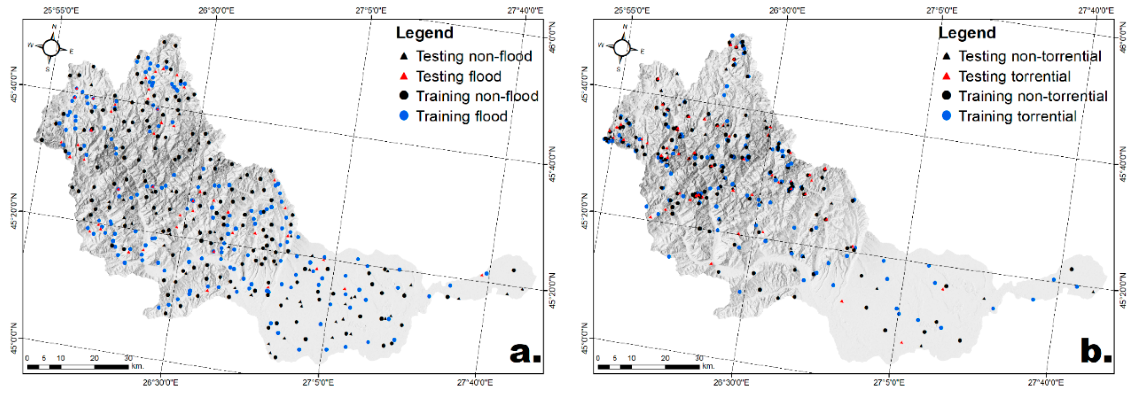
In order to compute the proposed models, we created a database which contains the historical flood locations from 1970–2012 and the locations of the areas affected by torrentiality. The areas affected by torrentiality were identified based on satellite imagery and from the RUSLE (Revised Universal Soil Loss Equation) model, which contains the areas where soil is affected by water erosion [44]. The database contains the locations of 168 historical floods (Figure 2a) which were obtained from the National Administration “Romanian Waters” and 172 locations affected by torrentiality (Figure 2b). According to previous studies which use Machine Learning techniques [45,46,47,48,49,50], the training and testing data were split in a 70% ratio for the training samples and 30% for the testing samples. This step is important as the proposed models are trained on the training samples while the testing samples are used as a final evaluation/confirmation of the model created based on the training samples.

2.3. Flood and Flash-Flood Conditioning Variables

The selection of the flood and flash-flood conditioning variables represents a key step in running the proposed models. The present study proposes the use of 14 flood conditioning variables, used to compute the Flood Potential Index (FPI), and 13 flash-flood conditioning variables, used to compute the Flash-Flood Potential Index (FFPI). The 14 variables used for the FPI are as follows: slope, elevation, hydrological soil groups (HSG), slope aspect, elevation above channel (EaC), distance from rivers (DfR), saturated hydraulic conductivity (SHC), land-use, drainage density (DD), plan curvature (PLC), Topographic Position Index (TPI), Topographic Wetness Index (TWI), multi-annual precipitations (MaP) and the Convergence Index (CI). The 13 variables used for the FFPI are as follows: slope, profile curvature (PC), HSG, slope aspect, slope length and steepness factor (L-S factor), Curve number (CN), CI, land-use, soil erodibility by water (SEW), DD, TPI, TWI, and MaP.
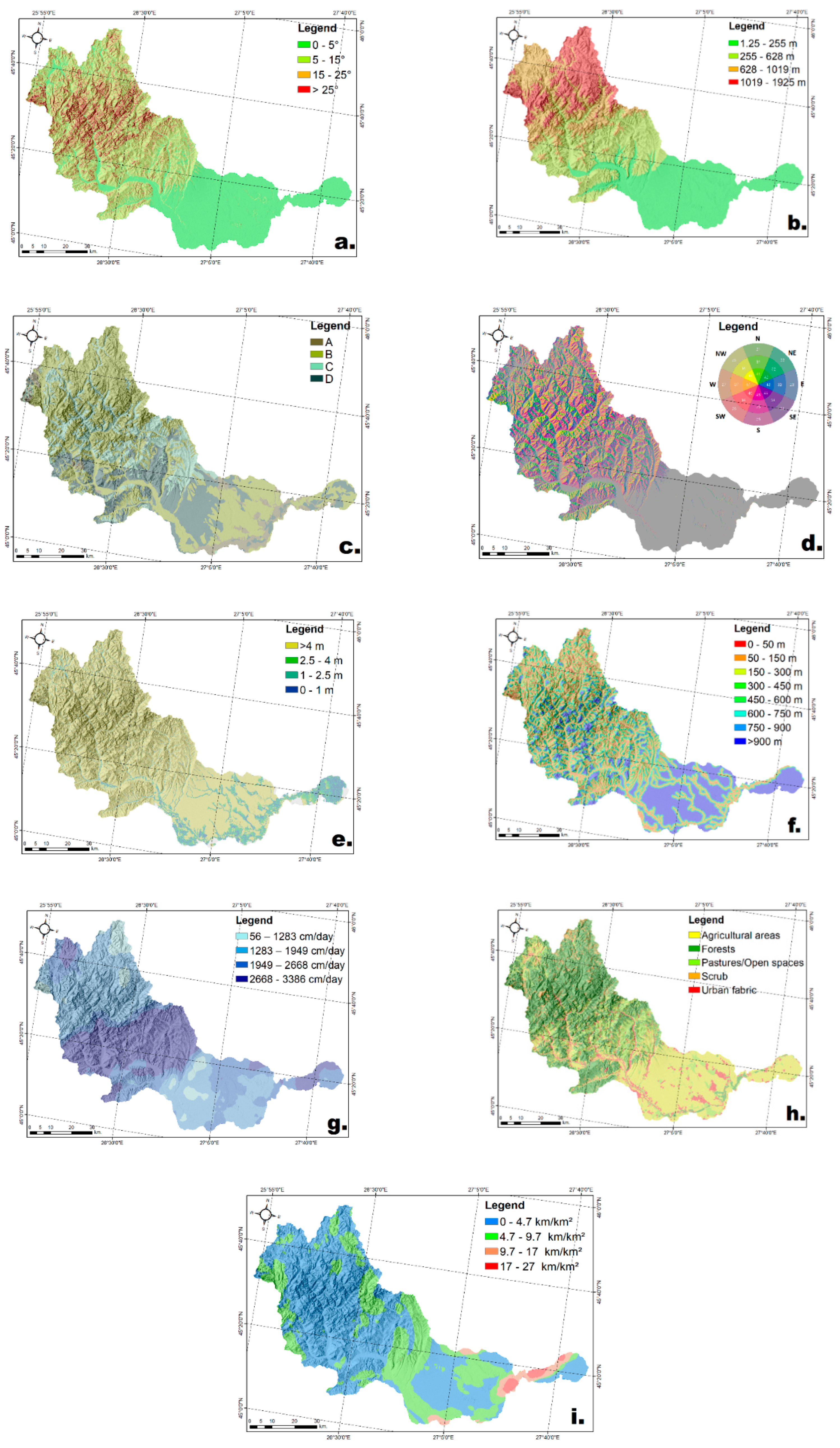
Most of the flood and flash-flood conditioning variables were derived from the Digital Elevation Model (DEM) which was extracted from the EU-DEM (European Digital Elevation Model) dataset with a global resolution of 25 m, which is available from the European Environment Agency (EEA). Therefore, the following variables were extracted from the DEM or from other outputs derived from it: slope, elevation, slope aspect, elevation above channel, distance from rivers, plan curvature, TPI, TWI, Convergence Index, profile curvature and L-S factor. The slope (Figure 3a) represents a very important flood or flash-flood conditioning variable, which is widely used in similar research, as its values influence the runoff process on steep slopes and the water accumulation process in areas with low slopes [40,41]. For both the FPI and FFPI, the slope was classified into five classes, as shown in Table 2 and Table 3. Most of the flood locations overlap the areas with slopes between 0 and 5°, representing 73.2% of the total flood pixels, while most of the areas affected by torrentiality overlap the slopes between 25–55°, representing 44.7% of the total torrential pixels.
The elevation (Figure 3b) was used for the analysis of the FPI, and was classified into five elevation classes, ranging from 1.29–1925 m. Most of the flood locations are in the elevation class between 1.29–55 m, representing 39.2% of the flood pixels. The hydrological soil groups (Figure 3c) were used in both indices, representing a very important flood conditioning variable with an impact on the water infiltration process.
The HSGs were created based on the curve number and the soil properties of the areas in which they overlap and were classified into four groups according to the National Engineering Handbook [51]. The four groups are as follows: A, B, C and D. The most predominant hydrological soil group was group C, covering 58.9% of the study area, followed by group B, with 19% coverage. The four groups have different hydraulic conductivity properties, and based on these, one can say that group A has a high infiltration rate and a low runoff whilst group D has a low infiltration rate and a high runoff potential. Group A soils have a hydraulic conductivity of over 40 μm/s and have the lowest runoff potential of the four groups. Also, when thoroughly wet, they have a high infiltration rate. Group B soils have a hydraulic conductivity between 10–40 μm/s when thoroughly wet and have a low runoff potential. Group C soils have a slow water infiltration rate with hydraulic conductivity values between 1–10 μm/s and have a moderately high runoff potential. Group D soils have the highest runoff potential and a low water infiltration rate when thoroughly wet, with a hydraulic conductivity of below 1 μm/s.
The slope aspect (Figure 3d) was classified into five slope orientation classes, with most of the catchment being covered by flat areas, representing 34.7%. Most of the flood locations are located on the flat areas, representing 52.9% of the flood pixels, whereas the areas affected by torrentiality are located on slopes with a northwest and easterly orientation, representing 29% of the torrential pixels. The importance of this variable is given by the fact that the slope orientation has a great influence on the humidity of the soil.
The elevation above channel variable (Figure 3e) was used to analyze the FPI, representing a suitable variable in the generation of floods, as the lower values are more subject to flooding than the areas with high values, and it was classified into four elevation classes. The distance from rivers (Figure 3f), as with the elevation above channel, was used in the analysis of the FPI, and was classified into eight distance classes from 0 to over 900 m. Over 46.4% of the flood locations overlap the distance class between 0 and 50 m, whilst the class ranging from 50 to 150 m overlaps 31.5% of the flood pixels.
The saturated hydraulic conductivity (Figure 3g) was derived from the dataset of the soil hydraulic properties of Europe, which is available to download from the European Soil Data Centre (ESDAC) and represents a variable which shows the amount of water that would infiltrate vertically through a saturated soil unit [52,53,54]. This factor is widely used in soil and water researches. The SHC was classified into four classes, ranging from 56–3386 cm/day. Most of the flood locations overlap the class between 2668–3386 cm/day, representing 40.4% of the flood pixels, while the class between 1283–1949 cm/day overlaps 30.9% of the flood pixels.
The land use (Figure 3h) represents a variable used to compute both indices which was derived from the CORINE Land Cover 2018 dataset and classified into five land-use classes. The forest land-use class covers most of the study area, representing 40.7% of the catchment’s surface, followed by the lands used for agricultural purposes, which cover 33.3% of the area. Over 25.5% of the flood pixels overlap the areas occupied by agricultural lands, while the areas most affected by the torrentiality phenomena overlap the forest areas where the slopes are the steepest, comprising 45.9% of the study area, followed by the areas covered by scrub, at 22.6%.
The land use and the deforested areas were corelated in order to get a better representation of our study area. The deforested areas were extracted from the Global Forest Change dataset, which is available from the Department of Geographical Sciences of the University of Maryland. The dataset offers us the forest changes from 2000 to 2018 and is available in a raster format. The forest change data are encoded with 0 for areas with no forest change and 1 for areas with forest change [55,56]. The deforested areas have been assigned the value of “open spaces with little or no vegetation”. The forest changes have been validated and partially corrected using Sentinel-2 satellite imagery, which is available from the European Space Agency (ESA). Around 14.9% of the torrential pixels overlap the areas covered by pastures, natural grasslands and open spaces with little or no vegetation.
The drainage density (Figure 3i) shows the drainage degree of the river network and represents a factor with a direct impact on the generation of floods [57,58]; it was classified into four classes from 0 to 27 km/km2. Around 55.9% of the flood pixels are in the class between 0–4.7 km/km2, whilst 42.2% of the flood pixels overlap the class between 4.7–9.7 km/km2. Over 98.8% of the torrential pixels overlap the class between 0 and 9.7 km/km2.
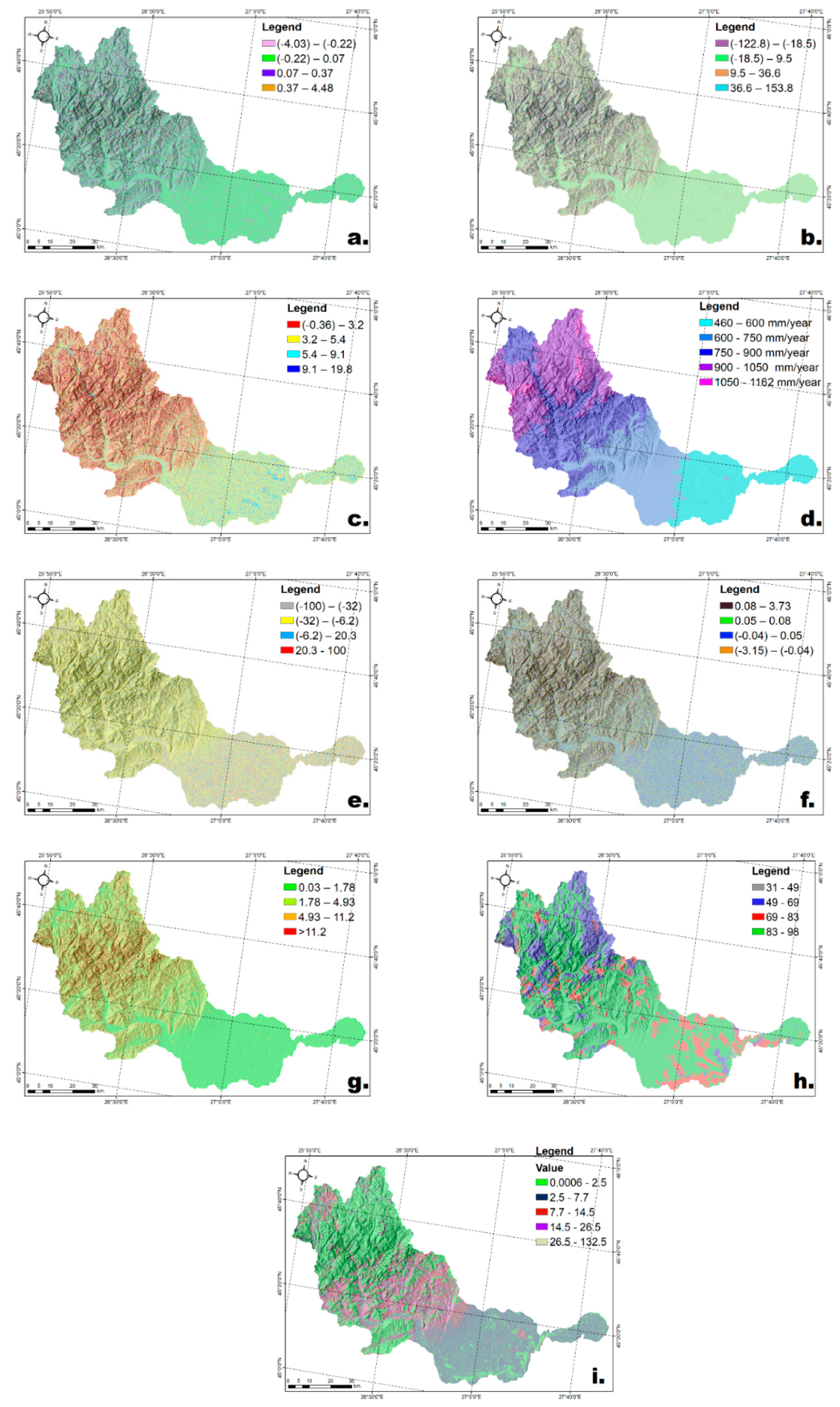
The plan curvature (Figure 4a) represents a flood conditioning variable used to compute the FPI, as shown by the areas with a divergent or a convergent flow. The variable was classified into four classes, ranging from (−4.03)–4.48. Over 71.4 of the flood pixels overlap the class between (−0.22)–0.07. The areas with values close to 0 indicate that the surface is linear, while the areas with negative values indicate that the surface is concave (convergent) and the positive values are convex (divergent) [59].
The Topographic Position Index (Figure 4b) indicates the altitude difference between the neighboring and focused cells in a DEM. The TPI was classified into four classes from (−122.8)–153.8. Positive values indicate that the altitude difference is higher than the one of the neighboring cells, whilst negative values indicate that the focused cell has a lower elevation than the neighboring cells, represented in general by valleys [60].
The Topographic Wetness Index (Figure 4c) was used in the computation of both indices. It represents a morphometric factor which indicates the moisture of the soil and shows the tendency of water distribution on soil [61]. The TWI depends on the topography of the area. This flood conditioning variable was classified into four classes ranging from (−0.36)–19.8. Over 44% of the flood pixels overlap the class between 3.2–5.4, whereas the areas affected by torrentiality are mostly present in the class between (−0.36)–3.2 and represent 69.7% of the study area.
The precipitation (Figure 4d) represents a flood and flash-flood conditioning variable which is widely used in flood research. The multi-annual precipitation was derived from the Global Climate dataset and classified into five classes ranging from 460–1162 mm/year. The MaP was used in the computation of both indices. The class 600–750 mm/year overlaps most of the flood pixels, at around 35.1%, followed by the class 750–900 mm/year, comprising 33.3% of the flood locations. Most of the torrential pixels—42.4%—overlap the class 900–1050 mm/year. The Convergence Index (Figure 4e) was derived from the DEM and was used for both the FPI and FFPI. This flood conditioning variable was classified in four classes ranging from (−100)–100. The negative values show that the structure of the surface is divergent and the values close to 0 indicate that the surface is planar, while the values close to 100 show that the surface is convergent.
The convergent areas are usually represented by channels, while the areas close to (−100) are represented by peaks or ridges. Around 83.9% of the flood pixels overlap the areas with values between (−32)–20.4, whilst 84.8% of the torrential pixels overlap the class between (−32)–(−6.2). The profile curvature (Figure 4f) was generated from the DEM and indicates the direction of the maximum slope of an area. The negative values indicate the fact that the surface is upwardly convex, the values close to 0 show that the surface is linear, and the areas with positive values are upwardly concave. The PC was classified into four curvature classes ranging from (−0.04) to 0.08.
The areas affected by torrentiality have an almost equal distribution in all classes, but the class between (−3.15)–(−0.04) overlaps 29% of the torrential pixels, making it the class with the highest percentage of torrential areas. The L-S factor (Figure 4g) or the slope length and steepness factor was extracted from the soil threat dataset from ESDAC [62]. The L-S factor resulted from the combination of the length of the slope and the slope angle. This flash-flood conditioning variable shows the effects of the slope steepness and is used to determine the areas prone to soil erosion. This factor was classified into four classes ranging between 0.03 and > 11.2. Most of the torrential pixels—around 58.1%—overlap the class between 4.93–11.2.
The curve number (CN; Figure 4h) represents a variable widely used in flash-flood research as it indicates the areas with high runoff values. The CN was classified into five classes and was used in the computation of the FFPI. The areas overlapping most of the torrential pixels cover 37.7% and range from 49–69, followed by the class 69–83 with 10.4% of the areas affected by torrentiality.
The soil erodibility by water factor (SEW) (Figure 4i) indicates areas where soil is prone to erosion caused by water. This factor used as inputs the topography of the area, soil types, rainfall, and land-use [44]. The SEW was classified into six erosion classes ranging from 0.0006–132.5 tons per ha/year and was derived from the RUSLE model. Over 63.7 of the torrential pixels overlap the class 0.0006–2.5 tons per ha/year, while the class 2.5–7.7 tons per ha/year overlaps 12.7% of the areas affected by torrentiality.

3. Flood and Flash-Flood Modelling Methods

3.1. Training and Testing the Models

A very important step in the present study is represented by the training of the models and testing them based on the locations in which flood or torrential phenomena are either present or not. These locations are called flood/torrential and non-flood/non-torrential areas. As mentioned before, the training and testing samples are split in a 70–30% ratio. The flood and torrential areas take the value of 1, whilst the non-flood and non-torrential areas are encoded with the value of 0. The training and testing samples also hold the values of the factors which overlap the locations with 1 and 0 and were extracted using the Extract Multi Values to Points tool in ArcGIS. The analysis of the samples was carried out in Microsoft Excel and in Weka 3.9 (open-source Machine Learning software). The resulting values were computed using ArcGIS, thus resulting in the hazard maps.

3.2. Frequency Ratio Model (FR)

The frequency ratio (FR) model represents a bivariate statistical method which is widely used in research for landslide and flood prediction mapping [24,29,31,32,47,63]. The present paper proposes the use of the FR model to map the areas prone to floods and flash-floods in the Buzău river catchment. The frequency ratio is a probabilistic model. It is simple, easy to understand and apply, and it aims to determine the ratio of the area in which the occurrence of a phenomenon is present in the study area and also the probability ratio of an occurrence to a non-occurrence for given attributes [64]. The FR method is based on the association of the flood and flash-flood conditioning variables and the locations of the historical floods or areas affected by torrentiality. The ratio is determined based on the analysis of the relation between the used factors and the flood and torrential locations and is shown in Table 2 and Table 3, alongside the prediction ratio (PR). High PR values show that the factor holds a high influence on the generation of floods or on the surface runoff. The PR was determined based on the spatial association of each variable within the training dataset for both indices and was calculated using Equation (1) [65]:
P R = ( S A m a x S A m i n ) ( S A m a x S A m i n )   m i n
where PR represents the prediction ratio of each variable and SA represents the maximum and the minimum spatial association between the variables and the flood or torrential locations. After determining the PR values of each factor, the FPI–FR and FFPI–FR models were computed in ArcGIS. The resulting weights for each index were compared and validated through a pairwise comparison matrix. Each raster of the flood conditioning variables was reclassified based on the relative frequency values (RF). The RF values were determined as follows:
R F = R + R t o t
where RF is the relative frequency, R+ is the ratio (+) or the positive ratio, and Rtot represents the sum of each positive ratio of a certain factor.
The FR model for the FPI and FFPI was determined using Equation (3) [29,63]:
F R = j = 1 n W i j
where FR represents the frequency ratio model applied for the FPI or FFPI, n is the number of flood conditioning variables, and Wij represents the weight of the class i of the parameter j.

3.3. Multilayer Perceptron Neural Networks (MLP)

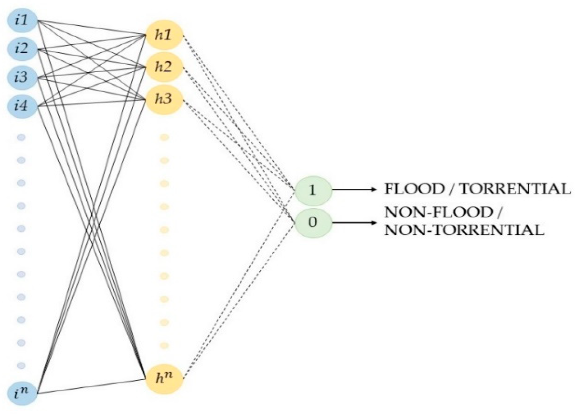
The Multilayer Perceptron is an artificial neural network (ANN) used in function approximation and pattern recognition and is made up of three components (Figure 5) [66]. Artificial neural networks represent a simple way to mimic the neural system of the human brain, in which, through various samples—in this case, the training samples—one can recognize data which were previously unseen, and make decisions and solve problems regarding the spatial relationship/association between input variables and the presence or absence of a certain phenomenon [34,67,68]. An MLP is based on the backpropagation algorithm—a supervised learning technique [66,69]. The neurons, represented by the variables/factors used in the analysis, are known as “input layers” and are connected to the “hidden layers” through a neural connection which holds the weights of the hidden layers. The connection of the input and output layers with each neuron of the hidden and output layers is represented by (4) [70]:
a j = i = 1 V ω i j ( 1 ) x i + ω 0 ( 1 ) ,   j = 1 ,   ,   N h
where Nh represents the neurons in the hidden layer, ωij(1) represents the weight of the connection between the neuron xi and the input layer and the neuron of the second layer, ωo(0) is the bias variable which prevents the parameter aj from becoming the value zero.
The hidden layers are also connected to the output layers through a neural connection which holds the output weights [33,71,72,73,74,75]. Initially, the weights of the connections hold random values until they intersect another connection—a phase in which they are multiplied by the associated weights and that intersection [34]. The interconnected neurons show the complex relationship between the input layers and the output layers—in this case, the flood/torrential or non-flood/non-torrential areas—and are also encoded with the values of 1 and 0 [34,72]. In order to avoid the overfitting of the neural network, the selection of the number of hidden neurons represents an important step as it controls the accuracy level of the network, proportionate to the noise level [76,77]. The number of neurons is determined based on Equation (5):
N h = 2 × V + 1
where Nh represents the number of hidden neurons and V represents the number of flood or flash-flood conditioning variables. Thus, the FPI–MLP model has 29 hidden neurons, whilst the FFPI–MLP has 27 hidden neurons. Based on the weight of each connection, the output layers generate an output decision with the values of 1 and 0. The output decisions are determined as follows:
O d = j = 1 V ω j ( 2 ) h j +   ω 0 ( 2 )
where Od is the output decision, ωj and ω0 represent the connection weights, and h is the hidden layer.

4. Results

4.1. Flood and Flash-Flood Hazard Mapping Using the Frequency Ratio (FR) Model

The first steps in computing the FR model for both the FPI and FFPI was to determine the positive ratio (Ratio +) and the prediction ratio (PR). These tasks were carried out in Microsoft Excel. After obtaining the values, the next step consisted of reclassifying each flood or flash-flood conditioning variable based on the Ratio + values, computing them using the raster calculator in ArcGIS, and multiplying them with the PR values. Hence, the resulting FPI–FR and FFPI–FR hazard maps are as shown in Figure 6 and Figure 7.
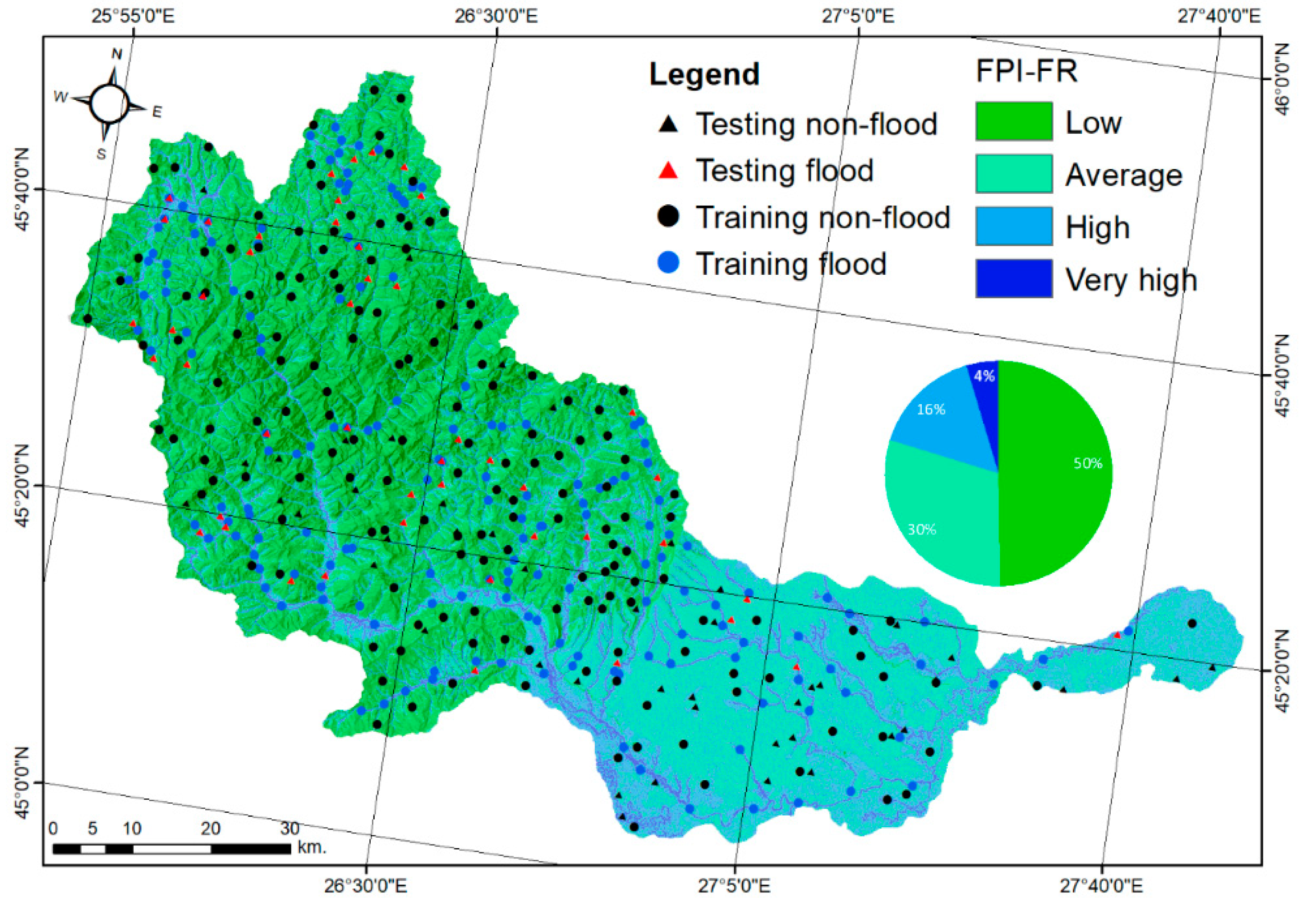
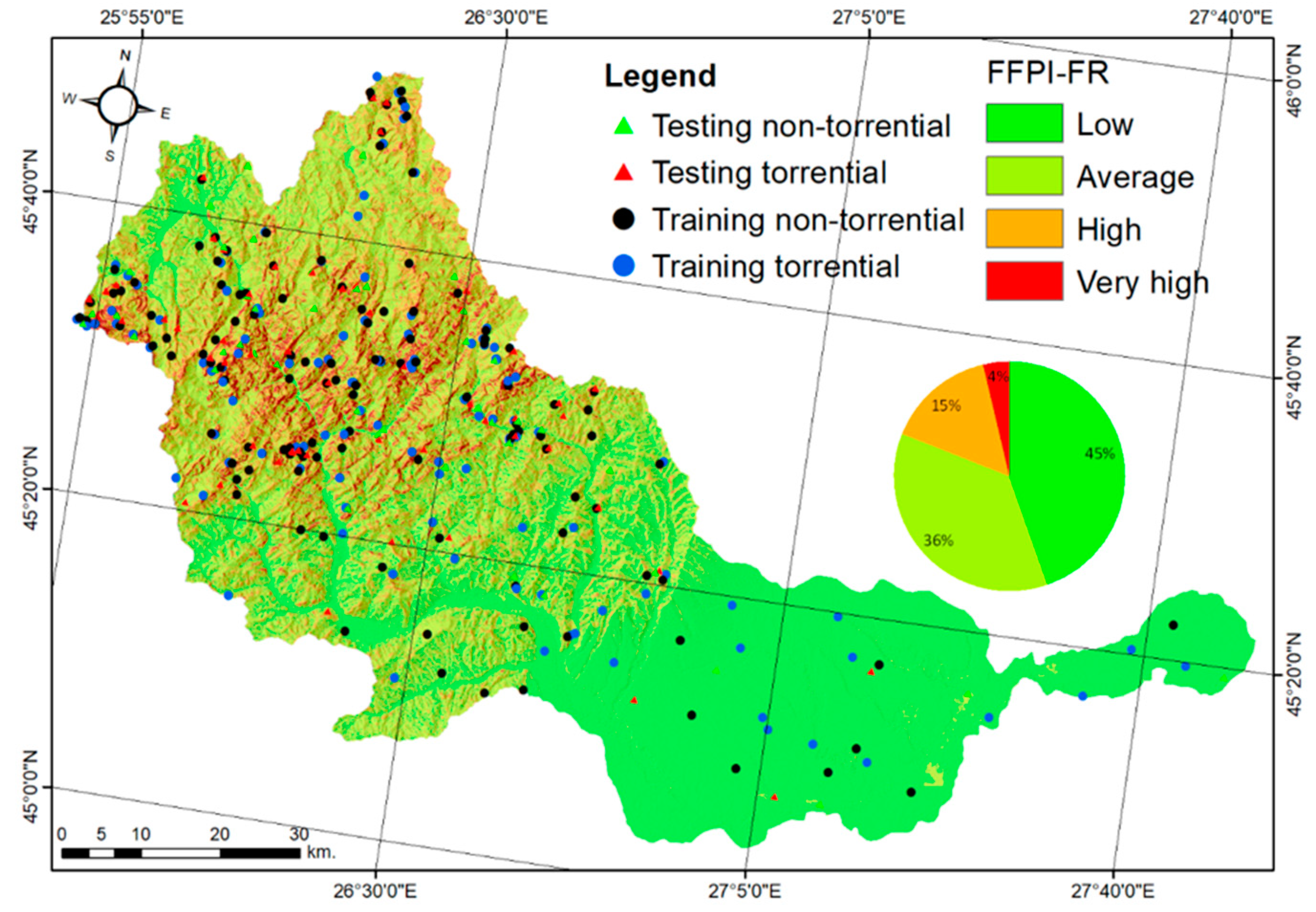
The FPI–FR and FFPI–FR models were classified into four hazard classes by using the Natural Breaks classification method in ArcGIS, as follows: low, average, high and very high. The resulting hazard map for the FPI–FR model shows that the low hazard class covers 50% of the catchment’s surface, the average class covers 30%, the high hazard class covers 16% of the area, and the very high hazard class covers 4%. The high and very high hazard classes are present in the lower catchment, where the slopes and altitudes are low, which is favorable for floods. The FFPI–FR model shows that 45% of the study area overlaps the low hazard class, 36% is in the average hazard class, 15% is in the high-hazard class, and the remaining 4% is characterized by areas with a very high hazard for flash-floods. The high and very high hazard classes are characteristic to areas with steep slopes in the upper basin, which are covered by pastures or areas with little or no vegetation.

4.2. Flood and Flash-Flood Hazard Mapping Using the Multilayer Percepton Neural Networks Model

The computation of the MLP model consisted in training the neural network with the flood locations for the FPI and with the torrential areas for the FFPI. This task was performed in Weka. The MLP model for each index was trained using 1000 maximum training epochs and 30 validation thresholds. The MLP model proposes the use of 30 validation thresholds in order to allow the algorithm to check for a decrease in error. If the model does not show a decrease in error, the training stops. Each model used a multi-start approach, which consists of running multiple models in parallel. The MLP model, used in the present study, uses a gradient descent optimization algorithm and a sigmoid activation function. The backpropagation algorithm uses the gradient descent to look for the minimum function each in weight space [78]. The sigmoid activation function used for the backpropagation algorithm is defined as follows, where c is an arbitrarily selected constant and 1/c is its reciprocal which is known as the temperature parameter [78]:
s c ( x ) =   1 1 + e c x  
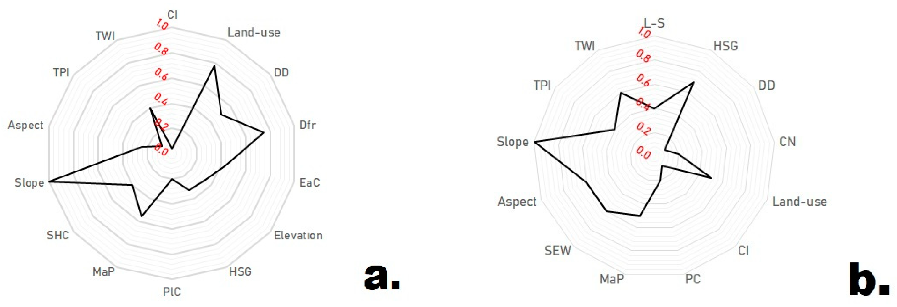
The resulting weights of each variable (Figure 8) were used to compute both indexes (Figure 9 and Figure 10). The variable importance for the Multilayer Perceptron was determined using the sensitivity analysis, which generates/computes the importance of the factors used in the neural network. The sensitivity analysis is generated automatically by the software after each run. The indices were computed in the same manner as for the FR model. The overall classification accuracy for the FPI–MLP is 90.91%, whilst for the FFPI–MLP, it is 86.03%. The percentage of correct observations per predicted values (0: non-flood/non-torrential areas; 1: flood/torrential) for the FPI–MLP are 86.41% for the non-flood areas and 90.52% for the flood areas, whilst for the FFPI–MLP, the percentages are 82.35% for the non-torrential areas and 89.72% for the torrential areas.
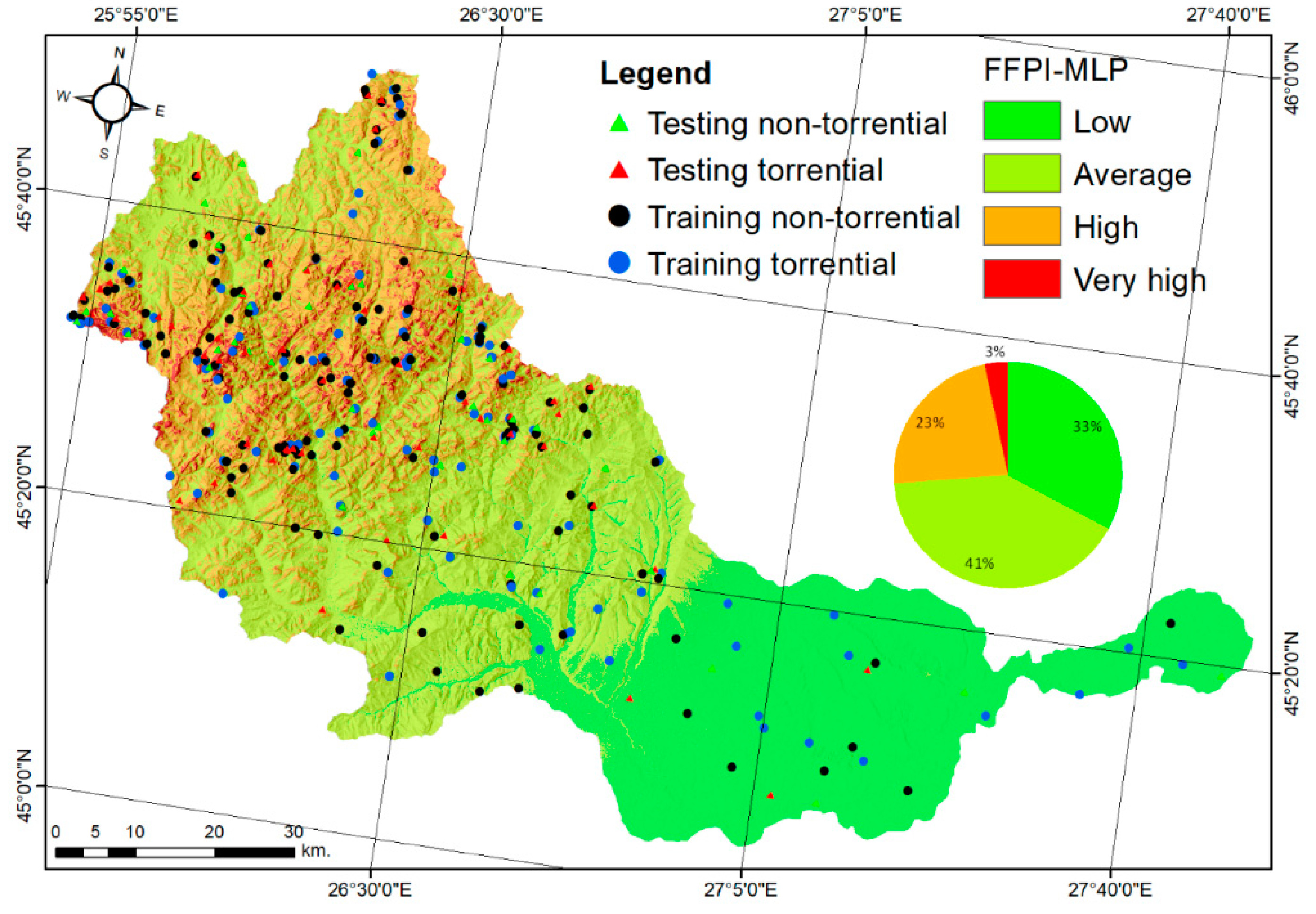
As for the FR model, the FPI and FFPI MLP model was classified into four hazard classes by using the Natural Breaks classification method. The FPI–MLP model shows that 37% of the study area is characterized by areas with a low hazard of floods, 41% by areas with an average-hazard, 15% by areas with a high hazard, and 7% was in the very high hazard class. As in the case of the FR model, the areas with average, high and very high hazard classes are located in the lower catchment. The slope, land use and distance from rivers were the variables with the highest importance values in the computation of the FPI–MLP model. The FFPI–MLP model shows that 41% of the study area is under the average flash-flood hazard class, which is predominant in the upper and middle part of the catchment. The low hazard class occupies 33% of the area, the high hazard occupies 23%, and the very high hazard class occupies 3% of the study area. The slope, multi-annual precipitation and the land use were the variables with the highest importance in the computation of the FFPI–MLP model.

4.3. Flood and Flash-Flood Mapping Using the Hybrid Integration between the Frequency Ratio and the Multilayer Perceptron Neural Networks

The hybrid integration between the frequency ratio and the Multilayer Perceptron consisted of integrating the FR positive ratio values with the variable importance resulting from the MLP model and computing them in ArcGIS. After the FR of each flood or flash-flood conditioning variable was computed and normalized, each factor was reclassified based on the Ratio + values. The values were normalized using Equation (8):
n v = ( v m i n ( r ) ) × ( m a x ( l ) m i n ( l ) ) m a x ( r ) m i n ( r ) + m i n ( l )
where nv is the standardized value, v represents the used variable, r is the limit of the range value, and l is the limit of the standardization range.
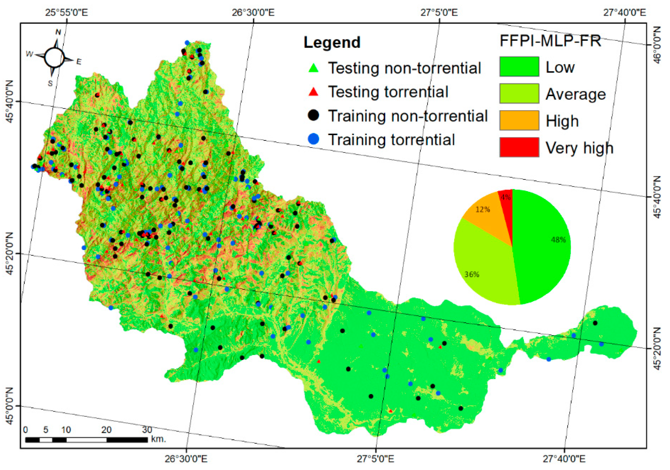
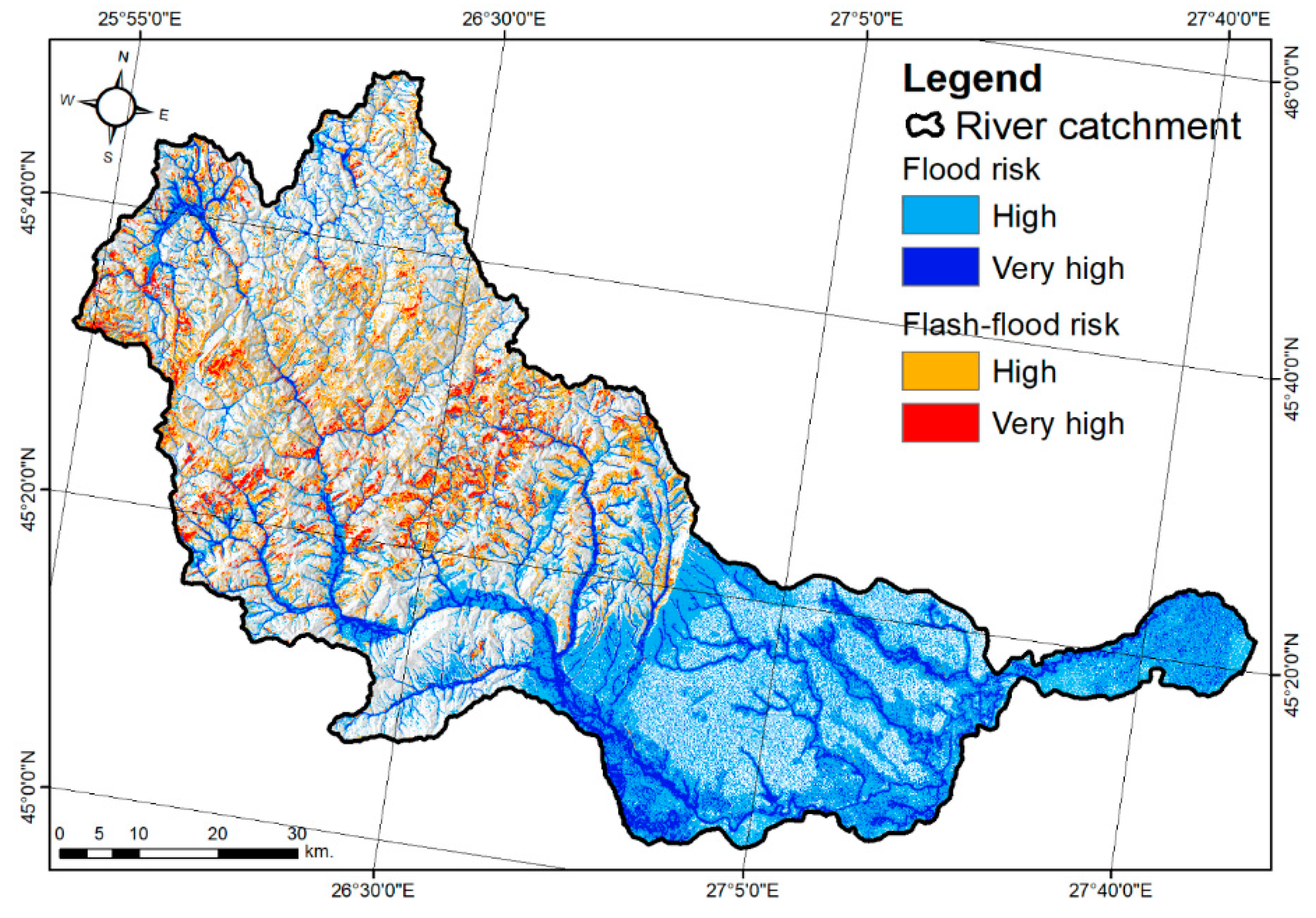
The role of hybrid models is to develop more accurate methods and reduce the potential disadvantages of the more traditional methods. The resulting hazard maps are shown in Figure 8 and Figure 9. The MLP–FR hybrid model was classified, as with the previous models, into four hazard classes by using the Natural Breaks method. The results indicate that for the FPI–MLP–FR model (Figure 11), 38% of the area are experience a low hazard of floods, while 37% have an average risk. The high and very high hazard classes represent 19% and 6% of the study area, respectively, and are located predominantly in the lower catchment in the proximity of the main water courses. The FFPI–MLP–FR (Figure 12) model shows that 55% of the catchment, especially in the lower catchment, is represented by areas with a low risk of flash floods. The average hazard class covers 36% of the study area, the high hazard class represents 12%, and the very high hazard class covers 4%. The very high values are mostly located in the middle part of the catchment. For both indices, the hybrid integration of both models proved to be the best-performing model. The flood and flash-flood hazard map (Figure 13) shows the areas which overlap the high and highest values of both indices.

4.4. Flood and Flash-Flood Model Performance Evaluation with ROC Curves

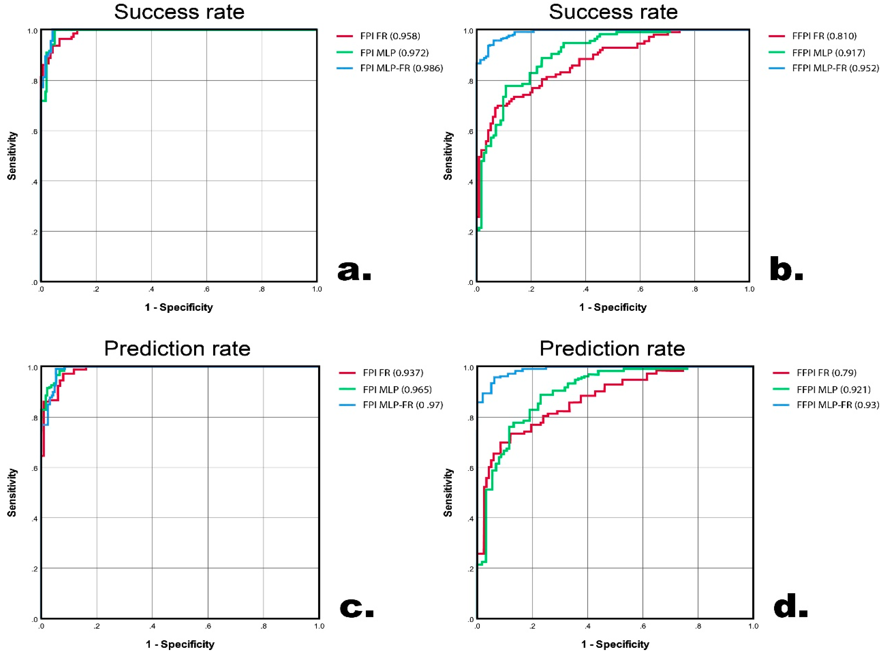
The performance evaluation of a model using the ROC (receiver operating characteristic) curve is a widely used method in research. The ROC curve represents a 2D plot which indicates the performance of a classifying system as the value of the discrimination cut-off is changed with respect to the predictor variable. The AUC (area under the curve) model represents a way to evaluate the testing ability in order to discriminate the true values. The ROC and AUC curves are made up from the sensitivity and specificity axes [79]. The success rate (Figure 14a,b) shows that the MLP–FR hybrid model was the best-performing model for both indices, with a value of 0.986 for the FPI and 0.952 for the FFPI, whilst the prediction rate (Figure 14c,d) shows the same trend. For both indices, the frequency ratio model proved to be the worst-performing model in terms of the success and prediction rate.

5. Discussion

Previous studies [80,81,82] have analyzed and presented flood forecasts at a resolution of 100 m; however, in order to determine and validate the areas prone to this natural hazard, it is crucial to have data at a high resolution [47]. Similar approaches have been tested using satellite imagery at different spatial resolutions [83], alongside various image processing techniques. Such approaches show great potential in areas where ground observations are rare or lacking. We consider that using a 25 m resolution does not affect the relevance of the obtained results.
The present study has shown that it is possible to obtain the areas prone to floods and flash-floods through Machine Learning techniques and statistical methods. Obtaining both indices through the spatial correlation of flood and flash-flood conditioning variables represents a useful tool for local authorities to assess the zones prone to these types of natural hazards. The methodology uses open-source technologies and data, which is relevant for researchers as the data-obtaining process represents an important obstacle in the development of relevant methodologies and studies in the analysis of various natural hazards. The present study proposes the computation of both indices which were highlighted in numerous studies aiming at determining the areas prone to these natural hazards. The outputs of the analysis make this study relevant, as other studies [32,35,36,38,40,47,72] propose the computation of only one index for creating hazard maps. The optimal split of the training and testing set used in the present paper was determined through successive testing using different split ratios—80–20 and 90–10. The 70–30 split ratio used in this study can only be generalized for similar datasets [84]. Thus, the developed models constitute a support in assisting decisions taken regarding the management and the expansion of public policies which aim at mitigating natural risks.
The obtained results show the need to complete similar approaches [47,72,85] with new variables, which will increase the relevance of the advanced modelling techniques.
The study shows the importance of developing methodologies for assessing areas vulnerable to floods and flash-floods as climatic events tend to intensify and the everchanging land use makes it imperative to develop new methodologies with new approaches and, more importantly, to obtain outputs.

6. Conclusions

The methodology developed in this study has been applied on the Buzău river catchment, known in Romania as one of the most affected catchments by these types of natural hazards. The methods used can be applied at a national level or on different river catchments, considering the increase in intensity of the climatic events and anthropic activities which nevertheless have a direct impact on the generation of floods and flash-floods. The flood hazard assessment by correlating the parameters of various factors which hold a direct impact on the generation of floods and flash-floods, with forest changes, historical flood locations and areas affected by torrentiality, represents a vital tool in the management of river catchments and for local authorities in order to implement public policies to prevent these types of natural hazards and avoid any human or economic losses [86,87,88].
A distributed hydrological model has the advantage of performing spatially refined simulations of hydrological components over a large area; thus, increasing the accuracy of data gives us the possibility to run the models on a large scale, with low costs and maximum benefits.

Author Contributions

Conceptualization, M.C.P.; Data curation, D.C.D.; Formal analysis, D.C.D.; Methodology, M.C.P. and D.C.D.; Project administration, C.C.D. and D.C.D.; Resources, C.C.D.; Software, M.C.P.; Supervision, D.P. and D.C.D.; Validation, D.C.D.; Writing—Original draft, M.C.P.; Writing—Review & editing, M.C.P., D.P. and D.C.D. These authors contributed equally to this work.

Funding

This research received no external funding.

Acknowledgments

This work was carried out with the logistical support of the project U.B– “Flood Analysis in Romania” grant number 1422/2019. We thank the anonymous reviewers for their suggestions, comments and careful reading of the manuscript.

Conflicts of Interest

The authors declare no conflict of interest.

References

  1. Assessment and Adaptation to Climate Change-Related Flood Risks: Oxford Research Encyclopedia of Natural Hazard Science—OI. Available online: https://oxfordindex.oup.com/view/10.1093/acrefore/9780199389407.013.278?lang=en,//oxfordindex.oup.com:443/view/10.1093/acrefore/9780199389407.013.278 (accessed on 19 August 2019).
  2. Didovets, I.; Krysanova, V.; Bürger, G.; Snizhko, S.; Balabukh, V.; Bronstert, A. Climate change impact on regional floods in the Carpathian region. J. Hydrol. Reg. Stud. 2019, 22, 100590. [Google Scholar] [CrossRef]
  3. Barriers and Guidelines for Public Policies on Climate Change Adaptation: A Missed Opportunity of Scientific Knowledge-Brokerage—Clar—2013—Natural Resources Forum—Wiley Online Library. Available online: https://onlinelibrary.wiley.com/doi/abs/10.1111/1477-8947.12013 (accessed on 31 August 2019).
  4. Barredo, J.I.; de Roo, A.; Lavalle, C. Flood risk mapping at European scale. Water Sci. Technol. 2007, 56, 11–17. [Google Scholar] [CrossRef] [PubMed]
  5. Paprotny, D.; Morales-Nápoles, O.; Jonkman, S.N. Efficient pan-European river flood hazard modelling through a combination of statistical and physical models. Nat. Hazards Earth Syst. Sci. 2017, 17, 1267–1283. [Google Scholar] [CrossRef] [Green Version]
  6. Massazza, G.; Tamagnone, P.; Wilcox, C.; Belcore, E.; Pezzoli, A.; Vischel, T.; Panthou, G.; Housseini Ibrahim, M.; Tiepolo, M.; Tarchiani, V.; et al. Flood Hazard Scenarios of the Sirba River (Niger): Evaluation of the Hazard Thresholds and Flooding Areas. Water 2019, 11, 1018. [Google Scholar] [CrossRef]
  7. Hennessey, R.; Pittman, J.; Morand, A.; Douglas, A. Co-benefits of integrating climate change adaptation and mitigation in the Canadian energy sector. Energy Policy 2017, 111, 214–221. [Google Scholar] [CrossRef]
  8. Dobler, C.; Bürger, G.; Stötter, J. Assessment of climate change impacts on flood hazard potential in the Alpine Lech watershed. J. Hydrol. 2012, 460, 29–39. [Google Scholar] [CrossRef]
  9. Zeleňáková, M.; Purcz, P.; Blišťan, P.; Vranayová, Z.; Hlavatá, H.; Diaconu, D.C.; Portela, M.M. Trends in Precipitation and Temperatures in Eastern Slovakia (1962–2014). Water 2018, 10, 727. [Google Scholar] [CrossRef]
  10. Yohe, G.W. Mitigative Capacity–the Mirror Image of Adaptive Capacity on the Emissions Side. Clim. Chang. 2001, 49, 247–262. [Google Scholar] [CrossRef]
  11. Filatova, T. Market-based instruments for flood risk management: A review of theory, practice and perspectives for climate adaptation policy. Environ. Sci. Policy 2013, 37, 227–242. [Google Scholar] [CrossRef]
  12. Balica, S.F.; Popescu, I.; Wright, N.G.; Beevers, L. Parametric and physically based modelling techniques for flood risk and vulnerability assessment: A comparison. Environ. Model. Softw. 2013, 41, 84–92. [Google Scholar] [CrossRef]
  13. Pradhan, B. Flood susceptible mapping and risk area delineation using logistic regression, GIS and remote sensing. J. Spat. Hydrol. 2009, 9, 1–18. [Google Scholar]
  14. Giustarini, L.; Chini, M.; Hostache, R.; Pappenberger, F.; Matgen, P. Flood Hazard Mapping Combining Hydrodynamic Modeling and Multi Annual Remote Sensing data. Remote Sens. 2015, 7, 14200–14226. [Google Scholar] [CrossRef] [Green Version]
  15. Gigović, L.; Pamučar, D.; Bajić, Z.; Drobnjak, S. Application of GIS-Interval Rough AHP Methodology for Flood Hazard Mapping in Urban Areas. Water 2017, 9, 360. [Google Scholar] [CrossRef]
  16. Balogun, A.-L.; Matori, A.-N.; Hamid-Mosaku, A.I. A fuzzy multi-criteria decision support system for evaluating subsea oil pipeline routing criteria in East Malaysia. Environ. Earth Sci. 2015, 74, 4875–4884. [Google Scholar] [CrossRef]
  17. Tehrany, M.S.; Pradhan, B.; Jebur, M.N. Spatial prediction of flood susceptible areas using rule based decision tree (DT) and a novel ensemble bivariate and multivariate statistical models in GIS. J. Hydrol. 2013, 504, 69–79. [Google Scholar] [CrossRef]
  18. Mukerji Aditya; Chatterjee Chandranath; Raghuwanshi Narendra Singh Flood Forecasting Using ANN, Neuro-Fuzzy, and Neuro-GA Models. J. Hydrol. Eng. 2009, 14, 647–652. [CrossRef]
  19. Pulvirenti, L.; Pierdicca, N.; Chini, M.; Guerriero, L. An algorithm for operational flood mapping from Synthetic Aperture Radar (SAR) data using fuzzy logic. Nat. Hazards Earth Syst. Sci. 2011, 11, 529–540. [Google Scholar] [CrossRef] [Green Version]
  20. Tehrany, M.S.; Pradhan, B.; Jebur, M.N. Flood susceptibility mapping using a novel ensemble weights-of-evidence and support vector machine models in GIS. J. Hydrol. 2014, 512, 332–343. [Google Scholar] [CrossRef]
  21. Campolo, M.; Soldati, A.; Andreussi, P. Artificial neural network approach to flood forecasting in the River Arno. Hydrol. Sci. J. 2003, 48, 381–398. [Google Scholar] [CrossRef]
  22. An Artificial Neural Network Model for Flood Simulation Using GIS: Johor River Basin, Malaysia | Springer Link. Available online: https://link.springer.com/article/10.1007/s12665-011-1504-z (accessed on 21 September 2019).
  23. Tiwari, M.K.; Chatterjee, C. Uncertainty assessment and ensemble flood forecasting using bootstrap based artificial neural networks (BANNs). J. Hydrol. 2010, 382, 20–33. [Google Scholar] [CrossRef]
  24. Rahmati, O.; Pourghasemi, H.R.; Zeinivand, H. Flood susceptibility mapping using frequency ratio and weights-of-evidence models in the Golastan Province, Iran. Geocarto Int. 2016, 31, 42–70. [Google Scholar] [CrossRef]
  25. Nandi, A.; Mandal, A.; Wilson, M.; Smith, D. Flood hazard mapping in Jamaica using principal component analysis and logistic regression. Environ. Earth Sci. 2016, 75, 465. [Google Scholar] [CrossRef]
  26. Lee, M.J.; Kang, J.; Jeon, S. Application of frequency ratio model and validation for predictive flooded area susceptibility mapping using GIS. In 2012 IEEE International Geoscience and Remote Sensing Symposium; IEEE: Munich, Germany, 2012; pp. 895–898. [Google Scholar]
  27. Evaluating the Application of the Statistical Index Method in Flood Susceptibility Mapping and Its Comparison with Frequency Ratio and Logistic Regression Methods: Geomatics, Natural Hazards and Risk. Available online: https://www.tandfonline.com/doi/full/10.1080/19475705.2018.1506509 (accessed on 31 August 2019).
  28. Cao, C.; Chen, J.; Zhang, W.; Xu, P.; Zheng, L.; Zhu, C. Geospatial Analysis of Mass-Wasting Susceptibility of Four Small Catchments in Mountainous Area of Miyun County, Beijing. Int. J. Environ. Res. Public Health 2019, 16, 2801. [Google Scholar] [CrossRef] [PubMed]
  29. Nohani, E.; Moharrami, M.; Sharafi, S.; Khosravi, K.; Pradhan, B.; Pham, B.T.; Lee, S.; Melesse, A. Landslide Susceptibility Mapping Using Different GIS-Based Bivariate Models. Water 2019, 11, 1402. [Google Scholar] [CrossRef]
  30. Zhang, T.; Han, L.; Chen, W.; Shahabi, H. Hybrid Integration Approach of Entropy with Logistic Regression and Support Vector Machine for Landslide Susceptibility Modeling. Entropy 2018, 20, 884. [Google Scholar] [CrossRef]
  31. Khan, H.; Shafique, M.; Khan, M.A.; Bacha, M.A.; Shah, S.U.; Calligaris, C. Landslide susceptibility assessment using Frequency Ratio, a case study of northern Pakistan. Egypt. J. Remote Sens. Space Sci. 2019, 22, 11–24. [Google Scholar] [CrossRef]
  32. Kumar Samanta, R.; Bhunia, G.; Shit, P.; Pourghasemi, H.R. Flood susceptibility mapping using geospatial frequency ratio technique: A case study of Subarnarekha River Basin, India. Model. Earth Syst. Environ. 2018, 4, 395–408. [Google Scholar] [CrossRef]
  33. Pham, B.T.; Tien Bui, D.; Prakash, I.; Dholakia, M.B. Hybrid integration of Multilayer Perceptron Neural Networks and machine learning ensembles for landslide susceptibility assessment at Himalayan area (India) using GIS. Catena 2017, 149, 52–63. [Google Scholar] [CrossRef]
  34. Gómez, H.; Kavzoglu, T. Assessment of shallow landslide susceptibility using artificial neural networks in Jabonosa River Basin, Venezuela. Eng. Geol. 2005, 78, 11–27. [Google Scholar] [CrossRef]
  35. Costache, R. Flash-flood Potential Index mapping using weights of evidence, decision Trees models and their novel hybrid integration. Stoch. Environ. Res. Risk Assess. 2019, 33, 1375–1402. [Google Scholar] [CrossRef]
  36. Wu, J.; Liu, H.; Wei, G.; Song, T.; Zhang, C.; Zhou, H. Flash Flood Forecasting Using Support Vector Regression Model in a Small Mountainous Catchment. Water 2019, 11, 1327. [Google Scholar] [CrossRef]
  37. Huang, W.; Cao, Z.; Huang, M.; Duan, W.; Ni, Y.; Yang, W. A New Flash Flood Warning Scheme Based on Hydrodynamic Modelling. Water 2019, 11, 1221. [Google Scholar] [CrossRef]
  38. Psomiadis, E.; Soulis, K.X.; Zoka, M.; Dercas, N. Synergistic Approach of Remote Sensing and GIS Techniques for Flash-Flood Monitoring and Damage Assessment in Thessaly Plain Area, Greece. Water 2019, 11, 448. [Google Scholar] [CrossRef]
  39. Dottori, F.; Martina, M.L.V.; Figueiredo, R. A methodology for flood susceptibility and vulnerability analysis in complex flood scenarios. J. Flood Risk Manag. 2018, 11, S632–S645. [Google Scholar] [CrossRef]
  40. Zaharia, L.; Costache, R.; Prăvălie, R.; Ioana-Toroimac, G. Mapping flood and flooding potential indices: A methodological approach to identifying areas susceptible to flood and flooding risk. Case study: The Prahova catchment (Romania). Front. Earth Sci. 2017, 11, 229–247. [Google Scholar] [CrossRef]
  41. Dou, J.; Yunus, A.P.; Tien Bui, D.; Sahana, M.; Chen, C.W.; Zhu, Z.; Wang, W.; Thai Pham, B. Evaluating GIS-Based Multiple Statistical Models and Data Mining for Earthquake and Rainfall-Induced Landslide Susceptibility Using the LiDAR DEM. Remote Sens. 2019, 11, 638. [Google Scholar] [CrossRef]
  42. Vojtek, M.; Vojteková, J. Flood Susceptibility Mapping on a National Scale in Slovakia Using the Analytical Hierarchy Process. Water 2019, 11, 364. [Google Scholar] [CrossRef]
  43. Miller, V.C. A quantitative geomorphic study of drainage basin characteristics in the Clinch Mountain area, Virginia and Tennessee. J. Geology 1953, 389–402. [Google Scholar]
  44. Panagos, P.; Borrelli, P.; Poesen, J.; Ballabio, C.; Lugato, E.; Meusburger, K.; Montanarella, L.; Alewell, C. The new assessment of soil loss by water erosion in Europe. Environ. Sci. Policy 2015, 54, 438–447. [Google Scholar] [CrossRef]
  45. Batista, G.; Prati, R.; Monard, M.C. A study of the behavior of several methods for balancing machine learning training data. ACM SIGKDD Explor. Newsl. 2004, 6, 20–29. [Google Scholar] [CrossRef]
  46. Shirzadi, A.; Shahabi, H.; Chapi, K.; Tien Bui, D.; Pham, B.; Shahedi, K.; Ahmad, B.B. A comparative study between popular statistical and machine learning methods for simulating volume of landslides. Catena 2017, 157, 213–226. [Google Scholar] [CrossRef]
  47. Cao, C.; Xu, P.; Wang, Y.; Chen, J.; Zheng, L.; Niu, C. Flash Flood Hazard Susceptibility Mapping Using Frequency Ratio and Statistical Index Methods in Coalmine Subsidence Areas. Sustainability 2016, 8, 948. [Google Scholar] [CrossRef]
  48. Li, X.; Yan, D.; Wang, K.; Weng, B.; Qin, T.; Liu, S. Flood Risk Assessment of Global Watersheds Based on Multiple Machine Learning Models. Water 2019, 11, 1654. [Google Scholar] [CrossRef]
  49. Mardani, M.; Mardani, H.; De Simone, L.; Varas, S.; Kita, N.; Saito, T. Integration of Machine Learning and Open Access Geospatial Data for Land Cover Mapping. Remote Sens. 2019, 11, 1907. [Google Scholar] [CrossRef]
  50. He, Q.; Xu, Z.; Li, S.; Li, R.; Zhang, S.; Wang, N.; Pham, B.T.; Chen, W. Novel Entropy and Rotation Forest-Based Credal Decision Tree Classifier for Landslide Susceptibility Modeling. Entropy 2019, 21, 106. [Google Scholar] [CrossRef]
  51. National Engineering Handbook Hydrology Chapters | NRCS. Available online: https://www.nrcs.usda.gov/wps/portal/nrcs/detailfull/national/water/manage/hydrology/?cid=STELPRDB1043063 (accessed on 8 August 2019).
  52. Jones, R.J.A.; Hiederer, R.; Rusco, E.; Montanarella, L. Estimating organic carbon in the soils of Europe for policy support. Eur. J. Soil Sci. 2005, 56, 655–671. [Google Scholar] [CrossRef] [Green Version]
  53. Tóth, B.; Weynants, M.; Nemes, A.; Makó, A.; Bilas, G.; Tóth, G. New generation of hydraulic pedotransfer functions for Europe. Eur. J. Soil Sci. 2015, 66, 226–238. [Google Scholar] [CrossRef]
  54. Mohsenipour, M.; Shahid, S. Estimation of Saturated Hydraulic Conductivity: A Review; Advances in Engineering Research; Nova Science Publishers Inc.: New York, NY, USA, 2016; Volume 15, Chapter 5; p. 181. [Google Scholar]
  55. Hansen, M.C.; Potapov, P.V.; Moore, R.; Hancher, M.; Turubanova, S.A.; Tyukavina, A.; Thau, D.; Stehman, S.V.; Goetz, S.J.; Loveland, T.R.; et al. High-Resolution Global Maps of 21st-Century Forest Cover Change. Science 2013, 342, 850–853. [Google Scholar] [CrossRef] [Green Version]
  56. Diaconu, D.C.; Andronache, I.; Pintilii, R.D.; Brețcan, P.; Simion, A.G.; Drăghici, C.C.; Gruia, K.A.; Grecu, A.; Marin, M.; Peptenatu, D. Using Fractal Fragmentation and Compaction Index in Analysis of the Deforestation Process in Bucegi Mountains Group, Romania. Carpathian J. Earth Environ. Sci. 2019, 14, 431–438. [Google Scholar]
  57. Pallard, B.; Castellarin, A.; Montanari, A. A look at the links between drainage density and flood statistics. Hydrol. Earth Syst. Sci. 2009, 13, 1019–1029. [Google Scholar] [CrossRef] [Green Version]
  58. Diaconu, D.C.; Andronache, I.; Ahammer, H.; Ciobotaru, A.M.; Zeleňáková, M.; Dinescu, R.; Pozdnyakov, A.V.; Alekseevna Chupikova, S. Fractal drainage model—A new approach to determinate the complexity of watershed. Acta Montan. Slovaca 2017, 22, 12–21. [Google Scholar]
  59. Wakeley, J.; Lichvar, R.; Noble, C.; Berkowitz, J. Regional Supplement to the Corps of Engineers Wetland Delineation Manual: Alaska Region (Version 2.0); US Army Corps of Engineers, U.S Army Engineer Research and Development Center: Vicksburg, MI, USA, 2011.
  60. De Reu, J.; Bourgeois, J.; Bats, M.; Zwertvaegher, A.; Gelorini, V.; De Smedt, P.; Chu, W.; Antrop, M.; De Maeyer, P.; Finke, P.; et al. Application of the topographic position index to heterogeneous landscapes. Geomorphology 2013, 186, 39–49. [Google Scholar] [CrossRef]
  61. Raduła, M.W.; Szymura, T.H.; Szymura, M. Topographic wetness index explains soil moisture better than bioindication with Ellenberg’s indicator values. Ecol. Indic. 2018, 85, 172–179. [Google Scholar] [CrossRef]
  62. Panagos, P.; Borrelli, P.; Meusburger, K. A New European Slope Length and Steepness Factor (LS-Factor) for Modeling Soil Erosion by Water. Geosciences 2015, 5, 117–126. [Google Scholar] [CrossRef] [Green Version]
  63. Yalcin, A.; Reis, S.; Aydinoglu, A.C.; Yomralioglu, T. A GIS-based comparative study of frequency ratio, analytical hierarchy process, bivariate statistics and logistics regression methods for landslide susceptibility mapping in Trabzon, NE Turkey. Catena 2011, 85, 274–287. [Google Scholar] [CrossRef]
  64. Bonham-Carter, G.F. Geographic Information Systems for Geoscientists: Modelling with GIS; Elsevier: Pergamon, Turkey, 1994; ISBN 978-1-4831-4494-8. [Google Scholar]
  65. Althuwaynee, O.F.; Pradhan, B.; Park, H.J.; Lee, J.H. A novel ensemble bivariate statistical evidential belief function with knowledge-based analytical hierarchy process and multivariate statistical logistic regression for landslide susceptibility mapping. Catena 2014, 114, 21–36. [Google Scholar] [CrossRef]
  66. Peponi, A.; Morgado, P.; Trindade, J. Combining Artificial Neural Networks and GIS Fundamentals for Coastal Erosion Prediction Modeling. Sustainability 2019, 11, 975. [Google Scholar] [CrossRef]
  67. Shiruru, K. An Introduction to Artificial Neural Network. Int. J. Adv. Res. Innov. Ideas Educ. 2016, 1, 27–30. [Google Scholar]
  68. Taravat, A.; Rajaei, M.; Emadodin, I.; Hasheminejad, H.; Mousavian, R.; Biniyaz, E. A Spaceborne Multisensory, Multitemporal Approach to Monitor Water Level and Storage Variations of Lakes. Water 2016, 8, 478. [Google Scholar] [CrossRef]
  69. Sánchez-Reolid, R.; García, A.S.; Vicente-Querol, M.A.; Fernández-Aguilar, L.; López, M.T.; Fernández-Caballero, A.; González, P. Artificial Neural Networks to Assess Emotional States from Brain-Computer Interface. Electronics 2018, 7, 384. [Google Scholar] [CrossRef]
  70. Wu, Q.; Lee, C.M. A Modified Leakage Localization Method Using Multilayer Perceptron Neural Networks in a Pressurized Gas Pipe. Appl. Sci. 2019, 9, 1954. [Google Scholar] [CrossRef]
  71. Deep Learning Multilayer Perceptron (MLP) for Flood Prediction Model Using Wireless Sensor Network Based Hydrology Time Series Data Mining—IEEE Conference Publication. Available online: https://ieeexplore.ieee.org/document/8319150 (accessed on 15 August 2019).
  72. Costache, R.; Tien Bui, D. Spatial prediction of flood potential using new ensembles of bivariate statistics and artificial intelligence: A case study at the Putna river catchment of Romania. Sci. Total Environ. 2019, 691, 1098–1118. [Google Scholar] [CrossRef] [PubMed]
  73. Castro, W.; Oblitas, J.; Santa-Cruz, R.; Avila-George, H. Multilayer perceptron architecture optimization using parallel computing techniques. PLoS ONE 2017, 12, e0189369. [Google Scholar] [CrossRef]
  74. Naganna, S.R.; Deka, P.C.; Ghorbani, M.A.; Biazar, S.M.; Al-Ansari, N.; Yaseen, Z.M. Dew Point Temperature Estimation: Application of Artificial Intelligence Model Integrated with Nature-Inspired Optimization Algorithms. Water 2019, 11, 742. [Google Scholar] [CrossRef]
  75. Allawi, M.F.; Binti Othman, F.; Afan, H.A.; Ahmed, A.N.; Hossain, M.S.; Fai, C.M.; El-Shafie, A. Reservoir Evaporation Prediction Modeling Based on Artificial Intelligence Methods. Water 2019, 11, 1226. [Google Scholar] [CrossRef]
  76. Improving Generalization of Artificial Neural Networks in Rainfall–Runoff Modelling/Amélioration de la Généralisation de Réseaux de Neurones Artificiels Pour la Modélisation Pluie-Débit: Hydrological Sciences Journal. Available online: https://www.tandfonline.com/doi/abs/10.1623/hysj.50.3.439.65025 (accessed on 18 September 2019).
  77. Gnana Sheela, K.; Deepa, S.N. Neural network based hybrid computing model for wind speed prediction. Neurocomputing 2013, 122, 425–429. [Google Scholar] [CrossRef]
  78. Rojas, R. Neural Networks: A Systematic Introduction; Springer: Berlin, Germany, 1996; ISBN 978-3-540-60505-8. [Google Scholar]
  79. Yang, S.; Berdine, G. The receiver operating characteristic (ROC) curve. Southwest Respir. Crit. Care Chron. 2017, 5, 34–36. [Google Scholar] [CrossRef]
  80. Advances in Pan-European Flood Hazard Mapping—Alfieri—2014—Hydrological Processes—Wiley Online Library. Available online: https://onlinelibrary.wiley.com/doi/abs/10.1002/hyp.9947 (accessed on 21 September 2019).
  81. Feyen, L.; Dankers, R.; Bódis, K.; Salamon, P.; Barredo, J. Fluvial flood risk in Europe in present and future climates. Clim. Chang. 2012, 112, 47–62. [Google Scholar] [CrossRef]
  82. Veijalainen, N. Estimation of Climate Change Impacts on Hydrology and Floods in Finland; Aalto University: Helsinki, Finland, 2012; ISBN 978-952-60-4614-3. [Google Scholar]
  83. Westerhoff, R.S.; Kleuskens, M.P.H.; Winsemius, H.C.; Huizinga, H.J.; Brakenridge, G.R.; Bishop, C. Automated global water mapping based on wide-swath orbital synthetic-aperture radar. Hydrol. Earth Syst. Sci. 2013, 17, 651–663. [Google Scholar] [CrossRef] [Green Version]
  84. Dobbin, K.K.; Simon, R.M. Optimally splitting cases for training and testing high dimensional classifiers. BMC Med. Genom. 2011, 4, 31. [Google Scholar] [CrossRef]
  85. Costache, R.; Zaharia, L. Flash-flood potential assessment and mapping by integrating the weights-of-evidence and frequency ratio statistical methods in GIS environment—Case study: Bâsca Chiojdului River catchment (Romania). J. Earth Syst. Sci. 2017, 126, 59. [Google Scholar] [CrossRef]
  86. Martins, B.; Nunes, A.; Lourenço, L.; Velez-Castro, F. Flash Flood Risk Perception by the Population of Mindelo, S. Vicente (Cape Verde). Water 2019, 11, 1895. [Google Scholar] [CrossRef]
  87. Silva, P.R.B.; Makara, C.N.; Munaro, A.; Schnitzler, D.; Diaconu, D.C.; Sandu, I.; Poleto, C. Risks associated of the waters from hydric systems Urban’s: The case of the rio Barigui, south of Brazil. Rev. Chim. 2017, 68, 1834–1842. [Google Scholar]
  88. Zeleňáková, M.; Gaňová, L.; Purcz, P.; Horský, M.; Satrapa, L.; Blišťan, P.; Diaconu, D.C. Mitigation of the Adverse Consequences of Floods for Human Life, Infrastructure, and the Environment. Nat. Hazards Rev. 2017, 18, 05017002. [Google Scholar] [CrossRef]
Figure 1. Location map.
Water 11 02116 g001
Figure 2. Location of flood and torrential areas (a) Flood/non-flood locations; (b) Torrential/non-torrential locations).
Water 11 02116 g002
Figure 3. (a) Slope, (b) elevation, (c) hydrological soil group (HSG), (d) slope aspect, (e) elevation above channel, (f) distance from rivers, (g) saturated hydraulic conductivity, (h) land use, (i) drainage density.
Water 11 02116 g003
Figure 4. (a) Plan curvature, (b) Topographic Position Index (TPI), (c) Topographic Wetness Index (TWI), (d) multi-annual precipitation, (e) Convergence Index, (f) profile curvature, (g) L-S factor, (h) curve number, (i) soil erodibility by water.
Water 11 02116 g004
Figure 5. Multilayer perceptron neural network diagram.
Water 11 02116 g005
Figure 6. Flood Potential Index (FPI)–frequency ratio (FR) spatial distribution.
Water 11 02116 g006
Figure 7. Flash-Flood Potential Index (FFPI)–FR spatial distribution.
Water 11 02116 g007
Figure 8. Variable importance for the FPI (a) and FFPI (b) in the Multilayer Perceptron Neural Network (MLP) model.
Water 11 02116 g008
Figure 9. FFPI–MLP spatial distribution.
Water 11 02116 g009
Figure 10. FFPI–MLP spatial distribution.
Water 11 02116 g010
Figure 11. FPI–MLP–FR spatial distribution.
Water 11 02116 g011
Figure 12. FFPI–MLP–FR spatial distribution.
Water 11 02116 g012
Figure 13. Flood and flash-flood hazard map.
Water 11 02116 g013
Figure 14. Reciever operating characteristic (ROC) curve and area under the curve (AUC) for the FPI (a,c) and FFPI (b,d) models.
Water 11 02116 g014
Table 1. General characteristics of the Buzău river catchment and its main sub-catchments.
RiverArea (km2)Length (km)Altitude (m)Slope Mean (°)Circularity Ratio
MinMeanMax
Buzău52643028516125040.24
Bâsca Roziliei7837639511101510150.28
Slănic425731205801240150.20
Bâsca Chiojdului340922396681340260.46
Câlnău2085785336700110.29
Sărățel18732141444900240.65
Table 2. Frequency and prediction ratio and the distribution of the flood locations and classes of each flood conditioning variable. EaC: elevation above channel; DfR: distance from rivers; SHC: saturated hydraulic conductivity; DD: drainage density; MaP: multi-annual precipitation.
Flood VariableVariable ClassesNo. of Flood Points% of Flood PointsClass Area% of Class AreaRatio (+)Prediction Ratio (PR)
Slope25–5510.59%201,8733.39%0.175.84
15–25158.92%1,093,63818.39%0.48
5–152917.26%2,282,99438.40%0.44
0–5012373.21%2,366,73639.80%1.83
Elevation1019–19252514.88%989,28316.63%0.891.08
628–10192615.47%1,235,41420.77%0.74
255–6285130.35%1,567,08826.35%1.51
1.2–2556639.28%2,153,45636.22%1.08
HSGA3017.85%1,289,14121.68%0.821
B3219.04%1,071,38318.02%1.05
C9958.92%3,242,96954.54%1.08
D74.16%341,7485.74%0.72
Slope aspectNorth, northeast158.92%832,63514%0.632.15
Northwest, east1810.71%698,42616.28%1.05
Flat8952.97%2,065,77734.74%1.52
West, southeast1911.30%1,103,67418.56%0.60
South, southwest2716.07%974,72916.39%0.98
EaC> 47544.64%4,967,94183.56%0.533.82
2.5–41810.17%268,3714.51%2.37
1–2.52615.47%306,4065.15%3
0–14929.16%402,5206.77%4.30
DfR0–507446.42%526,8078.86%5.236.26
50–1505331.54%870,45716.64%2.15
150–3003017.85%1,094,31518.40%0.97
300–45074.16%816,60213.73%0.30
450–60042.38%632,70310.64%0.22
600–750--426,5497.17%-
750–900--312,7045.25%-
>900--1,265,10421.27%-
SHC56–128384.76%352,0865.92%0.801.41
1283–19495230.95%2,377,77739.99%0.77
1949–26684023.80%1,376,67923.15%1.02
2668–33866840.47%1,838,69930.92%1.30
Land useBroad-leaved forest, coniferous forest, mixed forest3923.21%2,421,99040.73%0.563.94
Scrub and/or herbaceous vegetation148.33%281,1004.72%1.76
Agricultural areas, moors and heathland, arable land 4325.59%1,983,85633.36%0.76
Pastures, natural grassland, open spaces with little or no vegetation3420.23%889,83014.96%1.35
Built-up areas3822.61%368,4656.19%3.64
DD0–4.79455.95%3,831,52164.44%0.882.86
4.7–9.77142.26%1,888,41131.76%1.33
9.7–1721.19%155,0262.60%0.45
17–2710.59%70,2831.18%0.50
PLC(−4.03)–(−0.22)74.16%319,1965.36%0.774.16
(−0.22)–0.0712071.42%3,776,54963.52%1.12
0.07–0.374124.40%1,614,63327.15%0.89
0.37–4.48--234,8633.95%-
TPI(−122.8)–(−18.5)7343.45%968,84016.26%2.665.87
(−18.5)–9.58248.80%3,607,79560.68%0.80
9.5–36.674.16%963,88916.21%0.25
36.6–153.863.57%404,7176.80%0.52
TWI(−0.36)–3.22514.88%2,226,33737.44%0.395.59
3.2–5.47444.04%2,652,03744.60%0.98
5.4–9.14526.78%882,42314.84%1.80
9.1–19.82414.28%184,4443.10%4.60
MaP460–6001810.71%1,166,21319.61%0.542.25
600–7505935.11%1,523,30725.62%1.37
750–9005633.33%1,627,72527.37%1.21
900–10503319.64%1,460,01924.55%0.79
1050–116221.19%167,9772.82%0.42
CI(−100)–(−32)74.16%452,7567.61%0.543.93
(−32)–(−6.2)10663.09%4,231,27771.17%0.88
(−6.2)–20.33520.83%981,65616.51%1.26
20.3–1002011.90%279,5524.70%2.53
Table 3. Frequency and prediction ratio and the distribution of the flood locations and classes of each flash-flood conditioning variable. PC: plan curvature; CN: curve number; CI: Convergence Index; SEW: soil erodibility by water.
Flood VariableVariable ClassesNo. of Torrential Points% of Torrential PointsClass Area% of Class AreaRatio (+)Prediction Ratio (PR)
Slope0–51911.04%2,366,73639.80%0.275.10
5–152514.53%2,282,99438.40%0.37
15–255117.26%1,093,63718.39%1.61
25–557773.21%201,8733.39%13.18
PC0.08–3.733922.67%970,99116.33%1.381
0.05–0.084425.58%1,803,19030.32%0.84
(−0.04)–0.053922.67%1,939,67632.62%0.69
(–3.15)–(–0.04)5029.06%1,231,38420.71%1.40
HSGA148.13%1,289,14121.68%0.371.79
B4928.48%1,071,38318.02%1.58
C9856.97%3,242,96954.54%1.04
D116.39%341,7485.74%1.12
Slope aspectNorth, northeast3319.18%832,63514%1.361.56
Northwest, east5029.06%698,42616.28%1.78
Flat179.88%2,065,77734.74%0.28
West, southeast4727.32%1,103,67418.56%1.47
South, southwest2715.69%974,72916.39%0.95
L-S0.03–1.782112.20%2,668,19144.87%0.274.19
1.78–4.933721.51%2,150,82336.17%0.59
4.93–11.210058.13%1,076,94518.14%3.20
>11.2148.13%49,2820.82%9.81
CN31–4931.74%29,8920.50%3.462.34
49–696537.79%1,033,83417.38%2.17
69–831810.46%797,02013.40%0.78
83–988650%4,084,49568.70%0.72
CI(–100)–(–32)84.65%452,7567.61%0.611.85
(–32)–(–6.2)14684.88%4,231,27771.17%1.19
(–6.2)–20.3158.72%981,65616.51%0.52
20.3–10031.74%279,5524.70%0.37
Land useBroad-leaved forest, coniferous forest, mixed forest7945.93%2,421,99040.73%1.123.39
Scrub and/or herbaceous vegetation3922.67%281,1004.72%4.49
Agricultural areas, moors and heathland, arable land 2413.95%1,983,85633.36%0.41
Pastures, natural grassland, open spaces with little or no vegetation2313.37%889,83014.96%0.89
Built-up areas74.06%368,4656.19%0.65
SEW0.0006–2.510963.37%2,771,62346.61%1.354.23
2.5–7.72212.79%2,004,06633.70%0.37
7.7–14.5116.37%763,90312.84%0.49
14.5–26.5137.55%341,9285.75%1.31
26.5–132.5179.88%63,7211.07%9.22
DD0–4.711667.44%3,831,52164.44%1.041.83
4.7–9.75431.39%1,888,41131.76%0.98
9.7–1710.58%155,0262.60%0.22
17–2710.58%70,2831.18%0.49
TPI(–122.8)–(–18.5)2011.62%968,84016.26%0.712.93
(–18.5)–9.58147.09%3,607,79560.68%0.77
9.5–36.62816.27%963,88916.21%1
36.6–153.84325%404,7176.80%3.67
TWI(–0.36)–3.212069.76%2,226,33737.44%1.863.32
3.2–5.43721.51%2,652,03744.60%0.48
5.4–9.1148.13%882,42314.84%0.54
9.1–19.810.58%184,4443.10%0.18
MaP460–600105.81%1,166,21319.61%0.292.96
600–7501911.04%1,523,30725.62%0.43
750–9005129.65%1,627,72527.37%1.08
900–10507342.44%1,460,01924.55%1.72
1050–11621911.04%167,9772.82%3.90