Automatic Web Procedure for Calculating Flood Flow Frequency


Abstract
1. Introduction
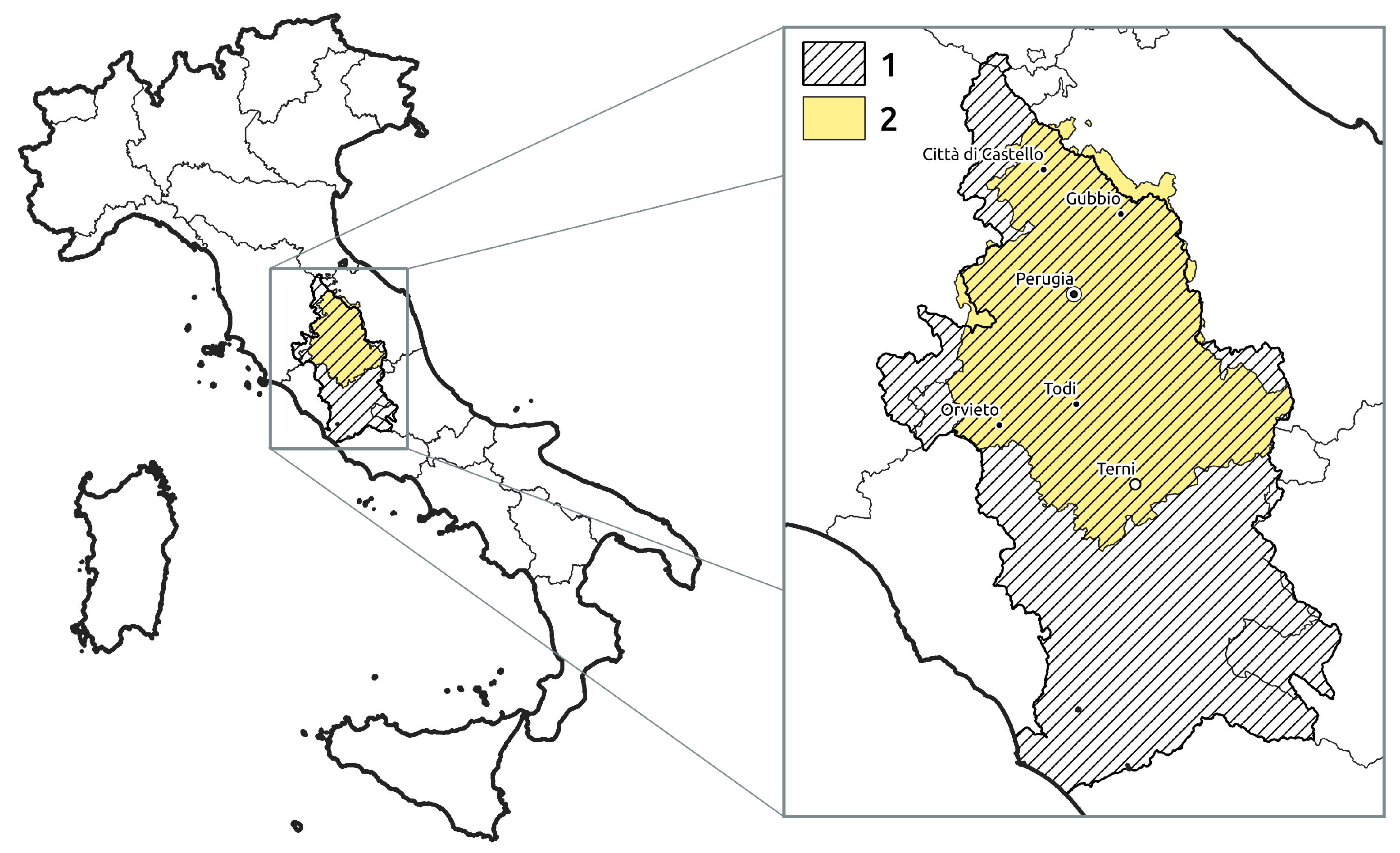
2. Description of Study Area
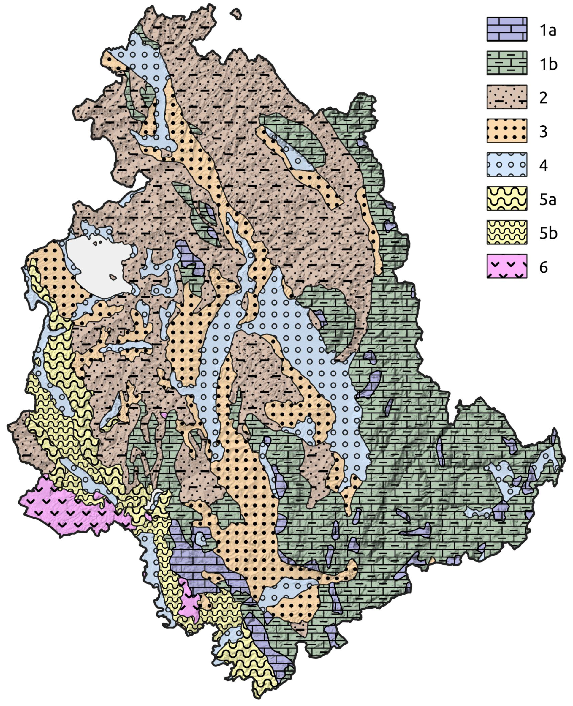
2.1. Geology
- Carbonate marine formations. They are mainly located in the eastern Apennine area. They can be subdivided into: a sequence of neritic and carbonate platforms facies, consisting mostly of limestones and a minor contribution of marls and dolomites (Late Triassic—Early Jurassic—1a in Figure 2), and a sequence of pelagic facies, consisting of micritic limestones, marly limestones and marls, sometimes with chert (Early Jurassic—Early Miocene—1b Figure 2).
- Siliciclastic marine formations (flysch). They were deposited by density flow processes in foreland basins and, in some cases, in thrust-top-basins. They consist of alternations of sandstones, arenaceous marls and mudrocks, with different ratios that depend on the depositional environment (submarine slope channel, upper fan, lower fan). These formations are dated, moving from west to east, from the Upper Cretaceous to the Upper Miocene.
- Unconsolidated deposits of lacustrine and fluvial-lacustrine continental environment. They were deposited in tectonic sedimentary basins. These are the oldest post-orogenic sediments and consists in gravels and conglomerates, sands, silts and clay. The age of these deposits ranges from the Lower Miocene to the Upper Pleistocene.
- Recent and terraced alluvial deposits. These are the most recent sediments and consist in gravels, sands, silts and clays. The age ranges from the Pleistocene to the Holocene.
- Unconsolidated deposits of marine and brackish-marine environment. They have been deposited at the same time as the continental ones (point 3), in the southwestern part of the studied area, in a coastal marine environment. A coastal/deltaic plain sequence of sands and conglomerates (5a in Figure 2) can be distinguished from a deeper marine environment sequence of clay (5b in Figure 1). The age of these deposits ranges from the Lower Pliocene to the Upper Pleistocene.
- Volcanic rocks. They are located in the most south-western portion of Umbria. They are connected to the activity of the Vulsini volcanic apparatus. They are formed by foidites, tephrites, latites, trachytes and phonolites. The age of these rocks refers to the Middle Pleistocene.
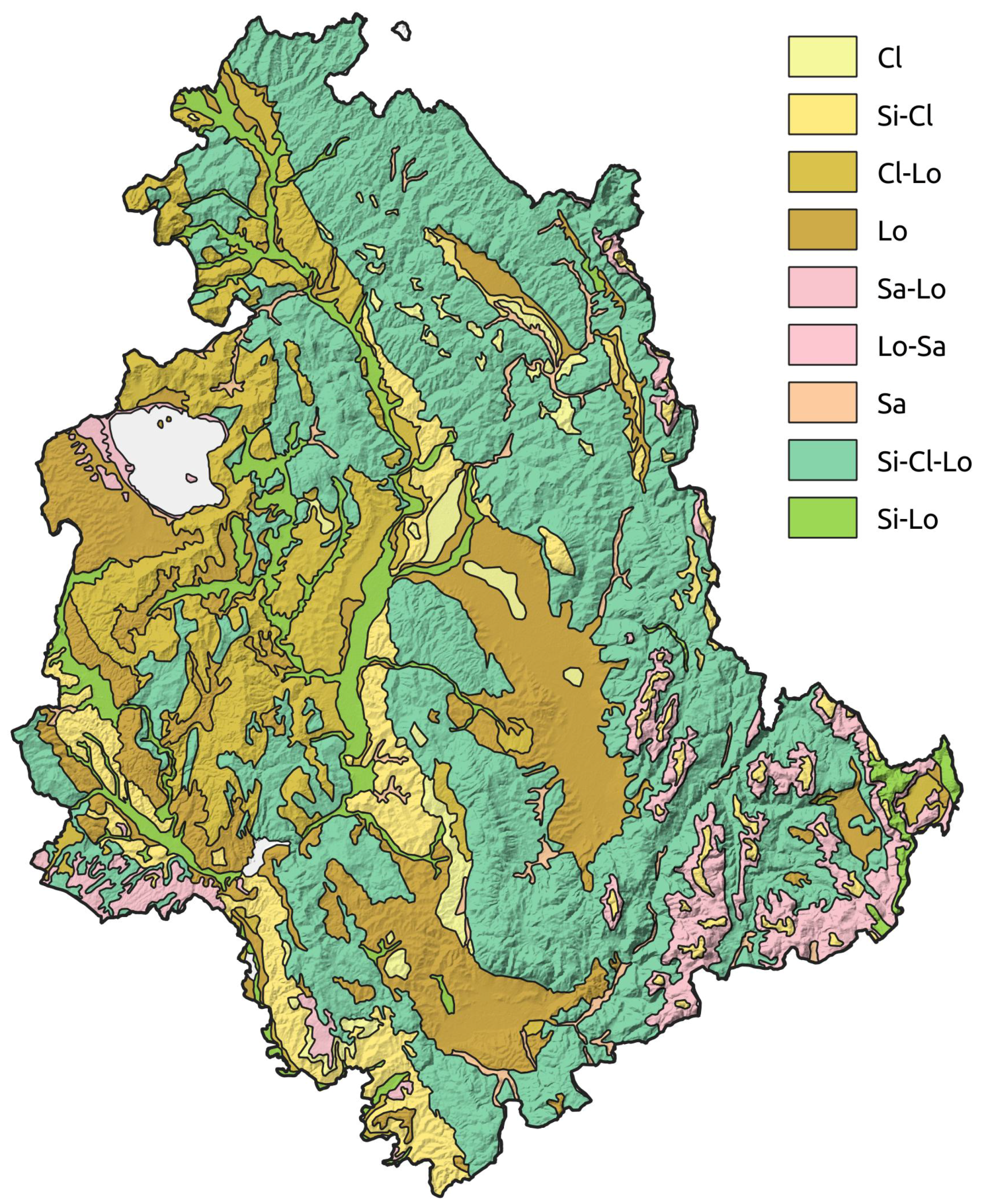
2.2. Soils
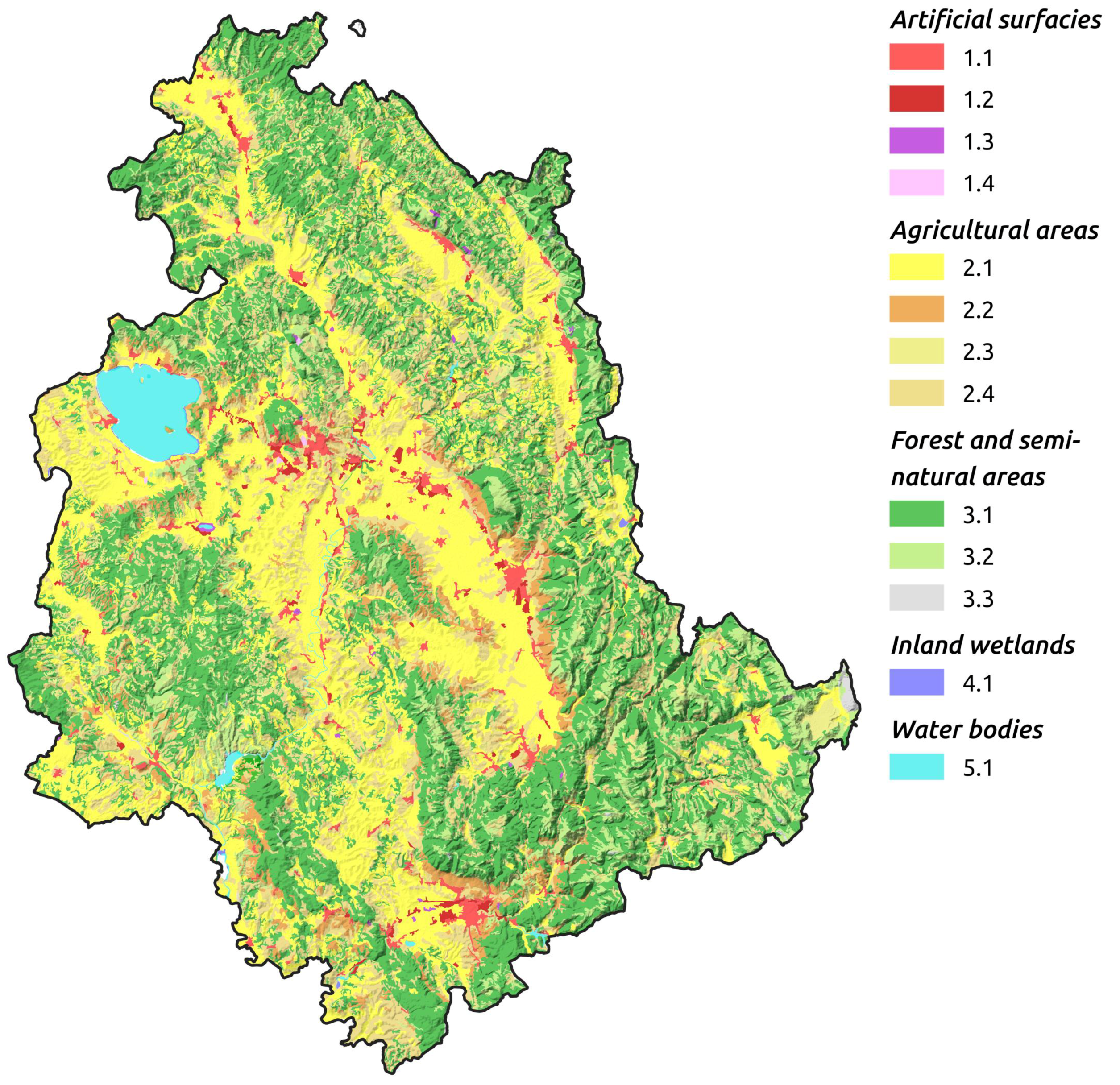
2.3. Morphological-Physiographic and Land Use Characteristics
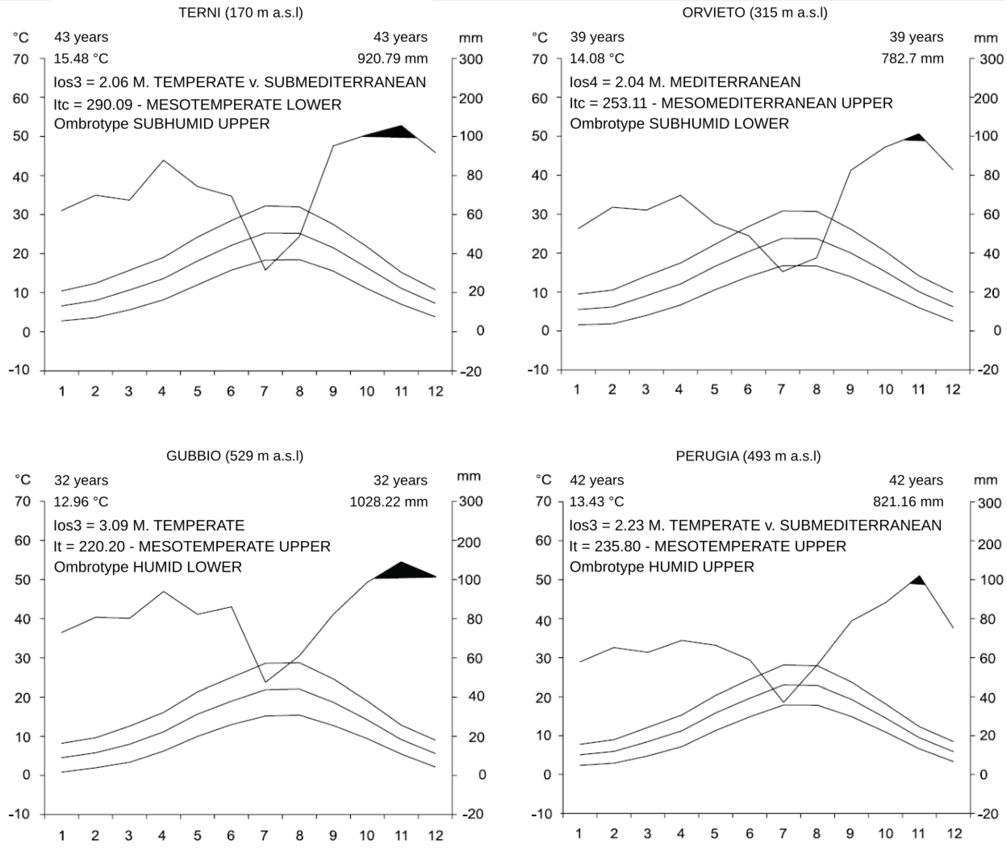
2.4. Climatic Conditions
3. Goal
4. Method: Procedure for Determining the Peak Flow According to the Flood Estimation Handbook of the Tiber River and Its Proposed Application
- the maximum flood occurs for rainfall duration equal to the run-off time of the contributing basin;
- the peak flow has the same return period as the rain that generated it;
- significant reservoirs are neglected along the hydrographic network: for an assigned hydrograph, the volume of net rain is set as equal to the volume of the peak flow.
- calculation of run-off time;
- calculation of local rainfall depth;
- calculation of areal rainfall depth;
- calculation of infiltration rate and, therefore, net rainfall;
- calculation of peak flow for a specific cross section.
4.1. Calculation of Run-Off Time
- Kirpich, for basins smaller then 10 km:with:
- = run-off time (hours)
- L = main channel length (km)
- = drop in elevation of main channel (m)
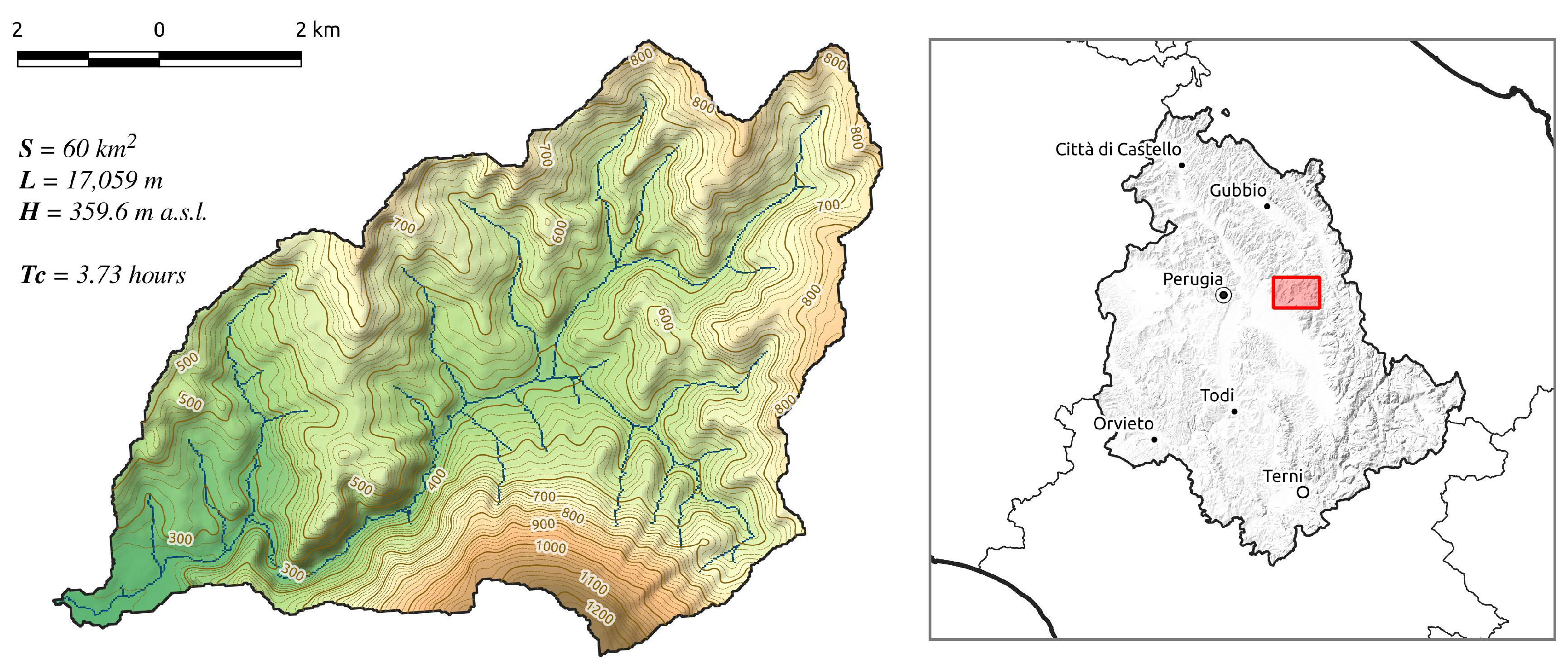
- Giandotti, for basins larger than 10 km:with:
- = run-off time (hours)
- S = basin area (km)
- L = main channel length (m)
- H = mean basin elevation (m a.s.l.).
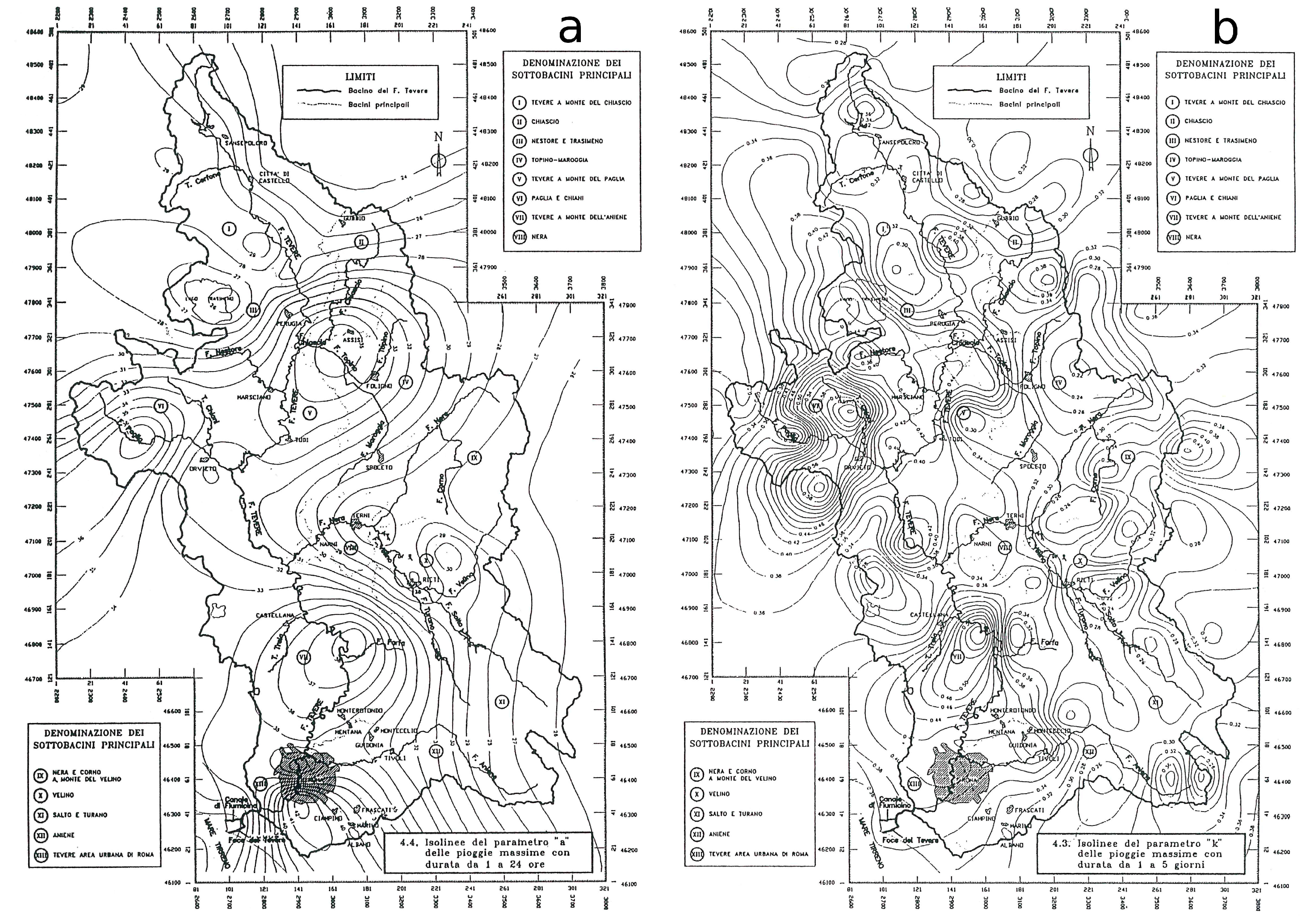
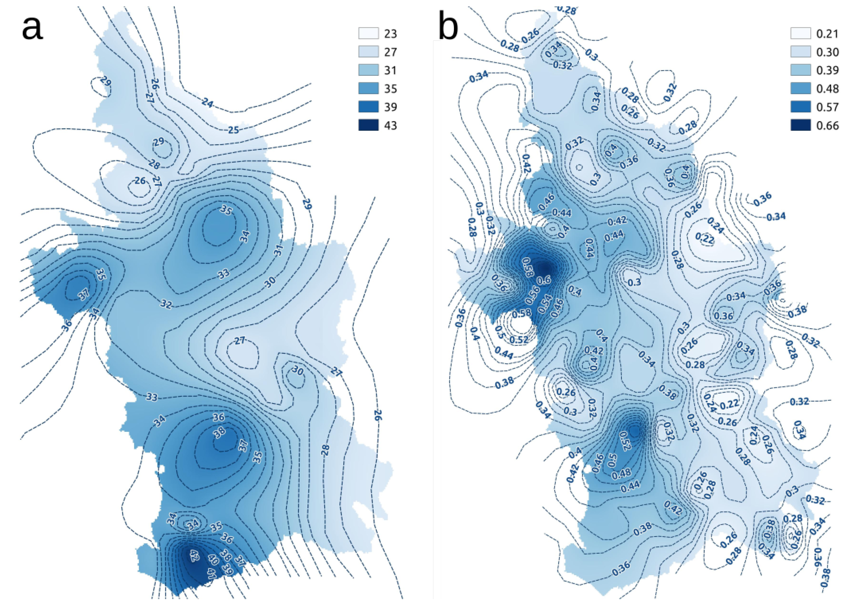
4.2. Calculation of Local Rainfall
- h = local rainfall depth in millimetres, lasting D with return period T
- D = duration of rainfall in hours
- RP = return period in years
- = parameters of the IDF curve
- K = coefficient of variation or relative standard deviation
4.3. Calculation of Areal Rainfall
- = areal rainfall depth (mm)
- h = local rainfall depth (mm)
- A = basin area (hectares)
- D = rainfall duration (hours)
4.4. Calculation of Net Rainfall: Procedure for Determining the Curve Number
- = ith area
- C = value of CN with respect to the ith area
- A = basin area (m)
- = net rainfall (mm)
- = areal rainfall (mm)
- = watershed’s maximum retention
- = average CN of the basin
4.5. Calculation of Peak-Flow
- = peak-flow (m/s)
- = net rainfall (mm)
- = run-off time (hours)
- A = basin area (ha)
5. The Calculation Code
- Identification of the catchment area;
- Evaluation of the run-off time and identification of the main channel;
- Calculation of the peak-flow;
- Generation of the report.
5.1. Identification of the Catchment Area
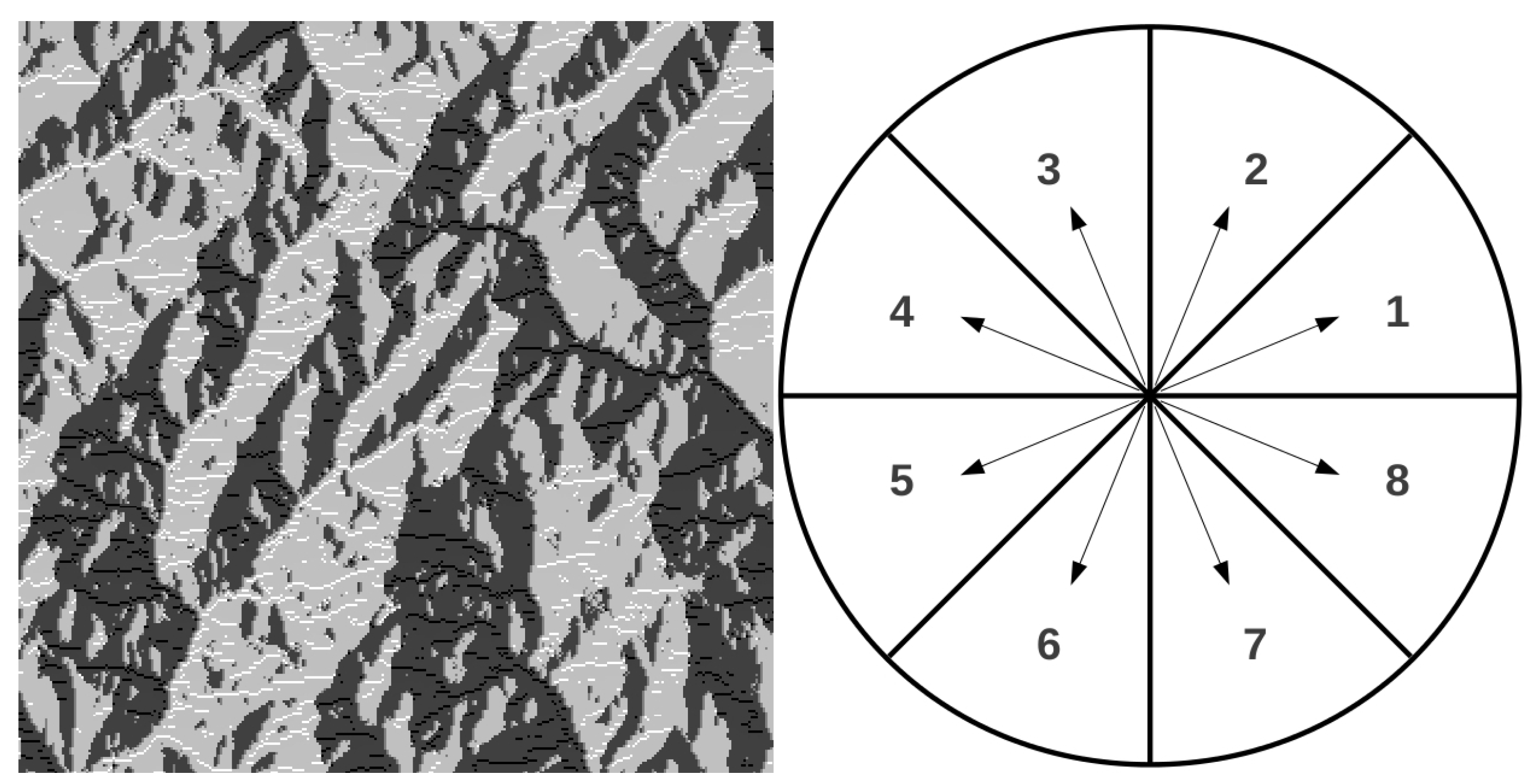
5.2. Evaluation of Run-Off Time and Identification of the Main Channel
- length of the main channel
- elevation drop of the main channel
- basin area
- mean basin elevation
- minimum basin elevation
- maximum basin elevation
5.3. Calculation of Peak-Flow
6. Discussion
6.1. Effects Analysis of the DEM Quality on the Estimated Peak Flow
- EU-DEM version 1.1, covering all Europe—25 m resolution and vertical accuracy of 2.9 m (https://land.copernicus.eu/imagery-in-situ/eu-dem)
- SRTM 1-arc second version V003, covering surfaces that lay between 60 degrees north latitude and 54 degrees south latitude—30 m resolution and declared vertical accuracy of 16 m (https://www2.jpl.nasa.gov/srtm/statistics.html).
- ASTER GDEM Version 2, covering surfaces that lay from 83 degrees north latitude to 83 degrees south—30 m resolution—the ASTER GDEM Validation Team assessed a vertical accuracy of 6.1 m in flat and open areas and 15.1 m in mountainous area largely covered by forest [31].
- TINITALY version 01, covering all Italy—10 m resolution and a vertical accuracy declared by the authors of 3.5 m [32].
6.2. Effects of Curve Number (CN) Value
6.3. Evaluation of the Accuracy of Estimated Peak Flow
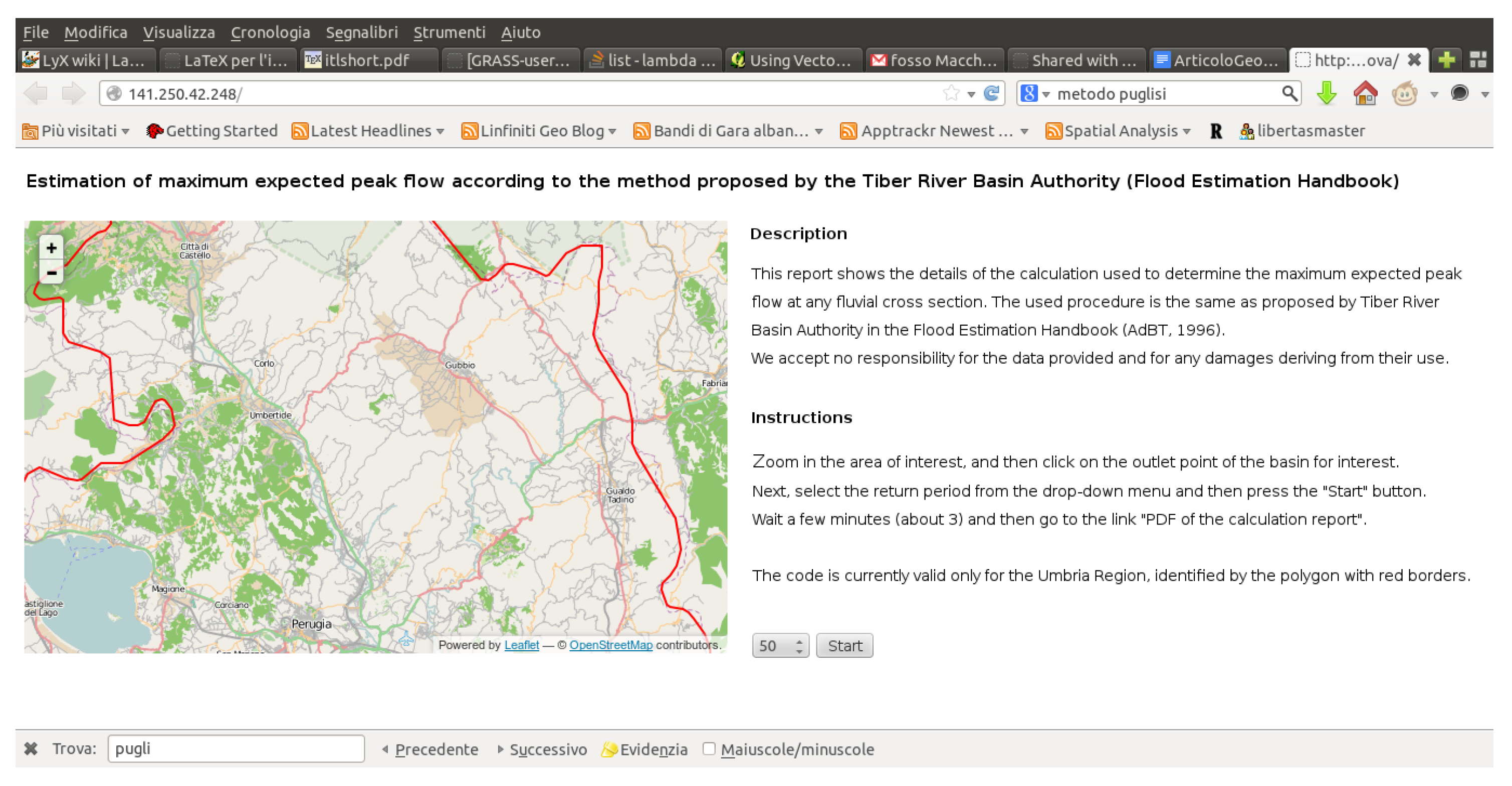
7. Web Tool
8. Conclusions and Future Developments
- the method is applied to small non-instrumented basins, where hydrological/hydraulic data are not available;
- the peak flow value is used for hydraulic engineering purposes, so a not excessive overestimation ensure higher safety standards.
Author Contributions
Funding
Acknowledgments
Conflicts of Interest
References
- Rodríguez-Iturbe, I.; Valdés, J.B. The geomorphologic structure of hydrologic response. Water Resour. Res. 1979, 15, 1409–1420. [Google Scholar] [CrossRef]
- Gupta, V.K.; Waymire, E.; Wang, C.T. A representation of an instantaneous unit hydrograph from geomorphology. Water Resour. Res. 1980, 16, 855–862. [Google Scholar] [CrossRef]
- Rodríguez-Iturbe, I.; González-Sanabria, M.; Bras, R.L. A geomorphoclimatic theory of the instantaneous unit hydrograph. Water Resour. Res. 1982, 18, 877–886. [Google Scholar] [CrossRef]
- Giannoni, F.; Roth, G.; Rudari, R. A procedure for drainage network identification from geomorphology and its application to the prediction of the hydrologic response. Adv. Water Resour. 2005, 28, 567–581. [Google Scholar] [CrossRef]
- Kumar, R.; Chatterjee, C.; Singh, R.D.; Lohani, A.K.; Kumar, S. Runoff estimation for an ungauged catchment using geomorphological instantaneous unit hydrograph (GIUH) models. Hydrol. Process. 2007, 21, 1829–1840. [Google Scholar] [CrossRef]
- Noto, L.V.; La Loggia, G. Derivation of a Distributed Unit Hydrograph Integrating GIS and Remote Sensing. J. Hydrol. Eng. 2007, 12, 639–650. [Google Scholar] [CrossRef]
- Brocca, L.; Melone, F.; Moramarco, T. Modellistica afflussi-deflussi di tipo continuo per la previsione delle piene su bacini dell’Alto-Medio Tevere. In Atti del XXXII Convegno Nazionale di Idraulica e Costruzioni Idrauliche; Farina: Palermo, Italy, 2010. [Google Scholar]
- Petroselli, A.; Grimaldi, S.; Alonso, G.; Nardi, F. Modelli afflussi deflussi per piccoli bacini idrografici non strumentati. In Atti del XXXII Convegno Nazionale di Idraulica e Costruzioni Idrauliche; Farina: Palermo, Italy, 2010. [Google Scholar]
- Grimaldi, S.; Petroselli, A.; Nardi, F.; Tauro, F. Analisi critica dei metodi di stima del tempo di corrivazione. In Atti del XXXII Convegno Nazionale di Idraulica e Costruzioni Idrauliche; Farina: Palermo, Italy, 2010. [Google Scholar]
- Domniţa, M.; Crăciun, I.; Haidu, I.; Magyari-Sáska, Z. GIS used for determination of the maximum discharge in very small basins (under 2 km2). WSEAS Trans. Environ. Dev. 2010, 6, 468–477. [Google Scholar]
- David, V.; Davidova, T. Methodology for flood frequency estimations in small catchments. Nat. Hazards Earth Syst. Sci. 2014, 14, 2655–2669. [Google Scholar] [CrossRef]
- Teresneu, C.C. Using gis for the determination of peak discharge in a small forested watershed. Bull. Transilv. Univ. Brasov. For. Wood Ind. Agric. Food Eng. Ser. II 2013, 6, 69. [Google Scholar]
- Dang, A.T.N.; Kumar, L. Application of remote sensing and GIS-based hydrological modelling for flood risk analysis: A case study of District 8, Ho Chi Minh city, Vietnam. Geomat. Nat. Hazards Risk 2017, 8, 1792–1811. [Google Scholar] [CrossRef]
- Uddin, K.; Gurung, D.R.; Giriraj, A.; Shrestha, B. Application of Remote Sensing and GIS for Flood Hazard Management: A Case Study from Sindh Province, Pakistan. Am. J. Geogr. Inf. Syst. 2013, 2, 1–5. [Google Scholar]
- Cheng, Q.; Ko, C.; Yuan, Y.; Ge, Y.; Zhang, S. GIS modeling for predicting river runoff volume in ungauged drainages in the Greater Toronto Area, Canada. Comput. Geosci. 2006, 32, 1108–1119. [Google Scholar] [CrossRef]
- Kulkarni, A.; Mohanty, J.; Eldho, T.; Rao, E.; Mohan, B. A web GIS based integrated flood assessment modeling tool for coastal urban watersheds. Comput. Geosci. 2014, 64, 7–14. [Google Scholar] [CrossRef]
- Eldho, T.I.; Zope, P.E.; Kulkarni, A.T. Chapter 12—Urban Flood Management in Coastal Regions Using Numerical Simulation and Geographic Information System. In Integrating Disaster Science and Management; Samui, P., Kim, D., Ghosh, C., Eds.; Elsevier: Amsterdam, The Netherlands, 2018; pp. 205–219. [Google Scholar]
- Autorità di Bacino del Fiume Tevere. Quaderno idrologico del Fiume Tevere. Tevere 1996, 1, 64. [Google Scholar]
- Pantaloni, M.; Bonomo, R.; Capotorti, F.; Compagnoni, B.; D’Ambrogi, C.; Di Stefano, R.; Galluzzo, F.; Graziano, R.; Martarelli, L.; Letizia Pampaloni, M.; et al. La nuova Carta Geologica d’Italia alla scala 1:500,000. Memorie Descrittive Carta Geologica d’Italia 2006, 1, 113–114. [Google Scholar]
- Giovagnotti, C.; Calandra, R.; Leccese, A.; Giovagnotti, E. I Paesaggi Pedologici e la Carta dei Suoli del l’Umbria; Camera di Commercio, Industria, Artigianato e Agricoltura di Perugia: Todi, Italy, 2003. [Google Scholar]
- Soil Science Division Staff. Soil Survey Manual; Handbook 18; Ditzler, C., Scheffe, K., Monger, H.C., Eds.; United States Department of Agriculture: Washington, DC, USA, 2017. [Google Scholar]
- Rivas-Martínez, S.; Rivas-Saenz, S.; Penas, A. Worldwide Bioclimatic Classification System; Backhuys Pub.: Kerkwerve, The Netherlands, 2002. [Google Scholar]
- Walter, H.; Lieth, H. Klimadiagramm-Weltatlas [World Climate Diagram]; Gustav Fischer: Jena, Germany, 1960. [Google Scholar]
- Rivas-Martínez, S.; Sánchez-Mata, D.; Costa, M. North American boreal and western temperate forest vegetation. Itinera Geobotanica 1999, 12, 5–316. [Google Scholar]
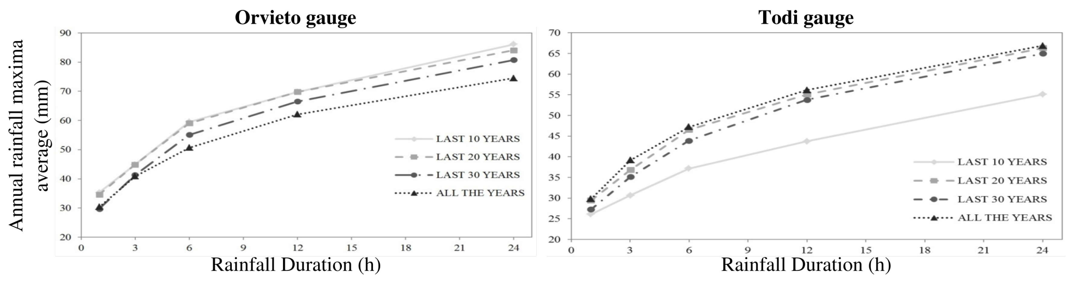
- Cifrodelli, M.; Corradini, C.; Morbidelli, R.; Saltalippi, C.; Flammini, A. The Influence of Climate Change on Heavy Rainfalls in Central Italy. Procedia Earth Planet. Sci. 2015, 15, 694–701. [Google Scholar] [CrossRef]
- Mitášová, H.; Mitáš, L. Interpolation by regularized spline with tension: I. Theory and implementation. Math. Geol. 1993, 25, 641–655. [Google Scholar] [CrossRef]
- Mockus, V. National Engineering Handbook Section 4, Hydrology; Technical Report; U.S. Department of Agriculture, Soil Conservation Service: Washington, DC, USA, 1969.
- Horton, R.E. Erosional Development of stream and their drainage basins; Hydrophysical approach to quantitative morphology. GSA Bull. 1945, 56, 275–370. [Google Scholar] [CrossRef]
- Jasiewicz, J.; Metz, M. A new GRASS GIS toolkit for Hortonian analysis of drainage networks. Comput. Geosci. 2011, 37, 1162–1173. [Google Scholar] [CrossRef]
- Cronshey, R. Urban Hydrology for Small Watersheds, 2nd ed.; Technical Report; U.S. Department of Agriculture, Soil Conservation Service, Engineering Division: Washington, DC, USA, 1986.
- Tachikawa, T.; Kaku, M.; Iwasaki, A.; Gesch, D.B.; Oimoen, M.J.; Zhang, Z.; Danielson, J.J.; Krieger, T.; Curtis, B.; Haase, J.; et al. ASTER Global Digital Elevation Model Version 2—Summary of Validation Results; Report; NASA: Washington, DC, USA, 2011; Available online: https://ssl.jspacesystems.or.jp/library/archives/ersdac/GDEM/ver2Validation/Summary_GDEM2_validation_report_final.pdf (accessed on 18 December 2018).
- Tarquini, S.; Isola, I.; Favalli, M.; Mazzarini, F.; Bisson, M.; Pareschi, M.T.; Boschi, E. TINITALY/01: A new Triangular Irregular Network of Italy. Ann. Geophys. 2007, 50, 407–425. [Google Scholar] [CrossRef]
- Elkhrachy, I. Vertical accuracy assessment for SRTM and ASTER Digital Elevation Models: A case study of Najran city, Saudi Arabia. Ain Shams Eng. J. 2017. [Google Scholar] [CrossRef]
- Di Francesco, S.; Biscarini, C.; Manciola, P. Characterization of a Flood Event through a Sediment Analysis: The Tescio River Case Study. Water 2016, 8, 308. [Google Scholar] [CrossRef]


| Orvieto | Terni | Perugia | Gubbio | |
|---|---|---|---|---|
| Observed years | 43 | 39 | 39 | 32 |
| Ic | 18.58 | 18.27 | 17.91 | 17.53 |
| Io | 4.96 | 4.63 | 5.09 | 6.61 |
| Ios1 | 1.25 | 1.28 | 1.61 | 2.77 |
| Ios2 | 1.59 | 1.43 | 2.04 | 2.47 |
| Ios3 | 2.06 | 1.72 | 2.33 | 3.09 |
| Ios4 | 2.04 | |||
| It | 286.70 | 251.75 | 235.80 | 220.20 |
| Itc | 290.09 | 253.11 |
| Orvieto | Terni | Perugia | Gubbio | |
|---|---|---|---|---|
| Macrobioclimate | mediterranean | temperate | temperate | temperate |
| Bioclimate | oceanic | oceanic | oceanic | oceanic |
| semicontinental | semicontinental | |||
| Bioclimatic variant | submediterranean | submediterranean | ||
| Thermotype | mesomediterranean | mesotemperate | mesotemperate | mesotemperate |
| lower | upper | upper | ||
| Ombrotype | subhumid lower | subhumid upper | subhumid upper | humid lower |
| 1st Level CORINE Land Cover | 2nd Level CORINE Land Cover | 3rd Level CORINE Land Cover | Soil Permeability | |||
|---|---|---|---|---|---|---|
| A | B | C | D | |||
| Artificial Land Cover | Urbanized Areas | Continuous urban fabric | 89 | 92 | 94 | 95 |
| Discontinuous urban fabric | 77 | 85 | 90 | 92 | ||
| Industrial or commercial units, road and rail networks | Industrial or commercial areas | 81 | 88 | 91 | 93 | |
| Road and rail networks and accessory spaces | 98 | 98 | 98 | 98 | ||
| Airports | 98 | 98 | 98 | 98 | ||
| Mineral extraction sites, dumps, construction sites | Mineral extraction sites | 51 | 68 | 79 | 84 | |
| Construction sites | 51 | 68 | 79 | 84 | ||
| Green urban areas | Sport and leisure facilities | 39 | 61 | 74 | 80 | |
| Land mainly occupied by agriculture, with significant areas of natural vegetation | Arable land | Non-irrigated arable land | 72 | 81 | 88 | 91 |
| Permanently irrigated land | Vineyards | 72 | 81 | 88 | 91 | |
| Olive groves | 72 | 81 | 88 | 91 | ||
| Natural grasslands | Natural grasslands | 30 | 58 | 71 | 78 | |
| Heterogeneous agricultural areas | Annual crops associated with permanent crops | 62 | 71 | 78 | 81 | |
| Cropping systems with permanent particles | 62 | 71 | 78 | 81 | ||
| Land mainly occupied by agriculture, with significant areas of natural vegetation | 62 | 71 | 78 | 81 | ||
| Wooded territories and semi-natural environments | Forestry areas | Broad-leaved forest | 25 | 55 | 70 | 77 |
| Coniferous forest | 45 | 66 | 77 | 83 | ||
| Mixed forest | 25 | 55 | 70 | 77 | ||
| Areas characterized by shrub and/or herbaceous vegetation | Pastures | 39 | 61 | 74 | 80 | |
| Moors and heathland | 39 | 61 | 74 | 80 | ||
| Sclerophyllous vegetation | 39 | 61 | 74 | 80 | ||
| Transitional woodland-shrub | 39 | 61 | 74 | 80 | ||
| Open areas with sparse or absent vegetation | Beaches, dunes, sands | 49 | 69 | 79 | 84 | |
| Bare rocks | 49 | 69 | 79 | 84 | ||
| Sparsely vegetated areas | 49 | 69 | 79 | 84 | ||
| Wetlands | Inland wetlands | Inland marshes | 100 | 100 | 100 | 100 |
| Water bodies | Continental waters | Water courses | 100 | 100 | 100 | 100 |
| Water basins | 100 | 100 | 100 | 100 | ||
| Res. | Vert. Acc. | S | L | H | ||||
|---|---|---|---|---|---|---|---|---|
| (m) | (m) | (ha) | (m) | (m a.s.l.) | (hours) | (m/s) | diff. (%) | |
| EU-DEM | 25 | 2.9 | 6024.74 | 17058.9 | 359.6 | 3.73 | 134.73 | / |
| SRTM | 30 | 16 | 6014.08 | 17126.5 | 357.4 | 3.75 | 134.15 | −0.4 |
| ASTER GDEM | 30 | 6.1 to 15 | 6006.90 | 15978.2 | 354.23 | 3.65 | 135.71 | 0.7 |
| TINITALY | 10 | 3.5 | 6092.81 | 17369.7 | 355.59 | 3.80 | 135.07 | 0.3 |
| Average CN | Basin Area | Local Rainfall | Areal Rainfall | Net Rainfall | Peak Flow |
|---|---|---|---|---|---|
| (ha) | (mm) | (mm) | (mm) | (m/s) | |
| 60.5 | 6025 | 104.4 | 98.1 | 18.3 | 81.8 |
| 69.1 | 6025 | 104.4 | 98.1 | 30.1 | 134.7 |
| 78.6 | 6025 | 104.4 | 98.1 | 46.3 | 207.3 |
| Years | T = 10 | T = 50 | T = 100 | T = 200 | T = 500 |
|---|---|---|---|---|---|
| Reference peak flow (m/s) | 12.52 | 88.04 | 116.86 | 148.46 | 191.98 |
| Modelled peak flow (m/s) | 53.43 | 108.23 | 134.73 | 162.69 | 201.60 |
| Difference (m/s) | 40.91 | 20.19 | 17.87 | 14.23 | 9.62 |
| Difference (%) | 326.8 | 22.9 | 15.3 | 9.6 | 5.0 |
© 2018 by the authors. Licensee MDPI, Basel, Switzerland. This article is an open access article distributed under the terms and conditions of the Creative Commons Attribution (CC BY) license (http://creativecommons.org/licenses/by/4.0/).
Share and Cite
De Rosa, P.; Fredduzzi, A.; Minelli, A.; Cencetti, C. Automatic Web Procedure for Calculating Flood Flow Frequency. Water 2019, 11, 14. https://doi.org/10.3390/w11010014
De Rosa P, Fredduzzi A, Minelli A, Cencetti C. Automatic Web Procedure for Calculating Flood Flow Frequency. Water. 2019; 11(1):14. https://doi.org/10.3390/w11010014
Chicago/Turabian StyleDe Rosa, Pierluigi, Andrea Fredduzzi, Annalisa Minelli, and Corrado Cencetti. 2019. "Automatic Web Procedure for Calculating Flood Flow Frequency" Water 11, no. 1: 14. https://doi.org/10.3390/w11010014
APA StyleDe Rosa, P., Fredduzzi, A., Minelli, A., & Cencetti, C. (2019). Automatic Web Procedure for Calculating Flood Flow Frequency. Water, 11(1), 14. https://doi.org/10.3390/w11010014