Confidence Regions for Multivariate Quantiles

Abstract

Multivariate quantiles are of increasing importance in applications of hydrology. This calls for reliable methods to evaluate the precision of the estimated quantile sets. Therefore, we focus on two recently developed approaches to estimate confidence regions for level sets and extend them to provide confidence regions for multivariate quantiles based on copulas. In a simulation study, we check coverage probabilities of the employed approaches. In particular, we focus on small sample sizes. One approach shows reasonable coverage probabilities and the second one obtains mixed results. Not only the bounded copula domain but also the additional estimation of the quantile level pose some problems. A small sample application gives further insight into the employed techniques.

1. Introduction

The track record of multivariate quantiles in hydrology is long and started with the papers by [1,2,3]. Quickly, a growing amount of literature on this topic with an application focus arose (see, e.g., [4,5,6]). A thorough overview of the current state of the art can be found in [7]. The notion of multivariate quantile we use in this paper is based on copulas. It has the nice feature that a $100\%·p$ multivariate quantile separates the copula domain into two sets, one comprising p, the other comprising $1-p$ of the total probability mass. Some theoretical aspects can be found in e.g., [8,9,10].

Not only the estimation of multivariate quantiles is important, but also an assessment of the estimation uncertainty. Confidence regions can be an essential tool for doing this. In contrast to pointwise confidence bands, confidence regions provide a holistic precision analysis of multivariate quantiles. For example, Refs. [11,12] construct confidence regions for multivariate quantiles based on highest density regions [13]. However, in principle, any approach for constructing confidence regions of level sets is applicable since the multivariate quantiles considered are specific level sets.

We attempt to fill this research gap and contribute to the existing literature on multivariate quantiles in several ways. First, we extend two recently developed approaches for construction of level set confidence regions by Mammen and Polonik [14] and Chen et al. [15] to the estimation problem at hand. Note that the multivariate quantiles considered here are level sets at specific levels of the copula. However, in contrast to the cited works, where the levels are known and fixed in advance, the level of the multivariate quantile has to be estimated. Second, we check the coverage probabilities of the extended methods by a simulation study in order to investigate their reliability. Finally, we apply the methods on a small sample of flood data to gain further insights.

The paper is structured as follows: The next section introduces copulas and the notion of multivariate quantiles used here. The confidence region approaches by Mammen and Polonik [14] and Chen et al. [15] are discussed in Section 3. Moreover, they are extended to multivariate quantile estimation. In Section 4, a simulation study is conducted in order to explore the strengths and weaknesses of the considered methods. The paper is concluded by an application on a small sample of flood data and a discussion of some further aspects.

2. Copulas and Multivariate Quantiles

This section introduces both copulas and the notion of multivariate quantiles we use throughout the paper. Additionally, the notation and some preliminaries are covered. According to Sklar’s theorem [16], every distribution function F of a continuous d-variate random variable $\mathbf{X}$ can be decomposed into a copula C and its univariate marginal distributions $F_1,\cdots ,F_d$ by

$$F(x_1,\cdots ,x_d)=C(F_1(x_1),\cdots ,F_d(x_d)).$$

This allows for separating the marginal distributions and the overall dependence structure of $\mathbf{X}$. The copula itself is a distribution function of the random variable $\mathbf{U}=(U_1,\cdots ,U_d)=(F_1(x_1),\cdots ,F_d(x_d))$. Note that the univariate components of $\mathbf{U}$ are uniformly distributed. A good theoretical introduction to copulas can be found, e.g., in [17,18,19]. An introduction for practical purposes can be found, e.g., in [8,20].

Let ${\mathbf{X}}_1,\cdots ,{\mathbf{X}}_n$ be an i.i.d. sample of a random vector $\mathbf{X}$ and let $x_{ij}$ be the ith component of the vector ${\mathbf{X}}_j$. The copula C of $\mathbf{X}$ may be estimated based on the so called pseudo observations ${\widehat{\mathbf{U}}}_j=\left({\widehat{u}}_{1j},\cdots ,{\widehat{u}}_{dj}\right)$, $j=1,\cdots ,n$. These can be obtained either by estimation of the marginal distributions ${\widehat{F}}_i(x)$, i.e.,

$${\widehat{\mathbf{U}}}_j=\left({\widehat{F}}_1(x_{1j}),\cdots ,{\widehat{F}}_d(x_{dj})\right),$$

or by rank transformation of the data, i.e.,

$${\widehat{\mathbf{U}}}_j=\frac{1}{n+1}(\mathrm{vector}\mathrm{of}\mathrm{component}-\mathrm{wise}\mathrm{ranks}\mathrm{of}{\mathbf{X}}_j\mathrm{in}{\mathbf{X}}_1,\cdots ,{\mathbf{X}}_n).$$

Note that estimation of the marginal distributions is prone to model misspecification [20]. Hence, a rank transformation is often preferable.

Using the pseudo observations ${\widehat{\mathbf{U}}}_j$, $j=1,\cdots ,n$, the copula can be estimated in different fashions. The estimator $\widehat{C}$ is called empirical copula and obtained by the empirical distribution of the pseudo observations

$$\widehat{C}(\mathbf{u})=\frac{1}{n}\sum _{j=1}^n{\mathbf{1}}_{\{{\widehat{\mathbf{U}}}_j\le \mathbf{u}\}}.$$

(1)

A second estimator ${\widehat{C}}_h$ that we use later on is based on kernel estimation. It is obtained by

$${\widehat{C}}_h(\mathbf{u})=\frac{1}{n}\sum _{i=1}^n{\mathbf{K}}_h({\mathrm{\Phi }}^{-1}(\mathbf{u})-{\mathrm{\Phi }}^{-1}({\widehat{\mathbf{U}}}_i)),$$

(2)

where ${\mathbf{K}}_h(\mathbf{x})=\mathbf{K}(\mathbf{x}/h)$ is the scaled version of a suitable multivariate kernel $\mathbf{K}$ and ${\mathrm{\Phi }}^{-1}$ is the inverse standard normal cumulative distribution function (CDF) applied component-wise. Using a multiplicative kernel, this estimator is investigated in [21]. The transformation ${\mathrm{\Phi }}^{-1}$ circumvents potential boundary issues that can arise in the copula domain ${[0,1]}^d$. It is also recommended in [18]. Apart from choosing a kernel, the estimator also requires a bandwidth parameter h. in this paper, we choose ${\mathbf{K}}_h$ to be a multiplicative multivariate Gaussian kernel and $h={\left(\frac{4}{d+2}n\right)}^{\frac{1}{d+4}}$, which is Silverman’s rule of thumb [22]. As will become clear later, these choices are particularly easy to work with and let us generate confidence regions in the original copula domain.

The Kendall distribution function $K_C:[0,1]⟼[0,1]$ [23,24,25] gives the probability that the copula C stays at or below a given level p, i.e.,

$$K_C(p)=\mathbb{P}(C(u_1,\cdots ,u_d)\le p).$$

Barbe et al. [23] show that the Kendall distribution function can be estimated non-parametrically from a sample of size n by

$${\widehat{K}}_C(p)=\frac{1}{n}\sum _{j=1}^n{\mathbf{1}}_{\{V_j\le p\}},$$

(3)

where $V_j=\frac{\#\{k\ne j|{\mathbf{X}}_k\le {\mathbf{X}}_j\}}{n-1}$. In addition to that, we need an estimator of the inverse of $K_C(p)$. For $0<p<1$, this is obtained by

$${\widehat{K}}_C^{-1}(p)=inf\{t|{\widehat{K}}_C(t)\ge p\}.$$

(4)

Furthermore, we define ${\widehat{K}}_C^{-1}(0)=0$ and ${\widehat{K}}_C^{-1}(1)=1$. Let $\mathrm{plim}$ denote convergence in probability. It can be shown that not only $\mathrm{plim}{\widehat{K}}_C(p)=K_C(p)$ for $p\in [0,1]$ [23], but also $\mathrm{plim}{\widehat{K}}_C^{-1}(p)=K_C^{-1}(p)$ for $p<1$ [26]. Moreover, ${\widehat{K}}_C$ is strongly consistent [27].

Using the previous concepts of copulas and the Kendall distribution function, we can now define the notion of multivariate quantiles we use in this paper. It has been used previously in, e.g., [7,9] and in a similar fashion in [10]. in the following, let $\mathcal{C}$ denote the class of copulas for which $K_C$ is strictly increasing and continuous.

Definition 1

([9]). For a copula $C\in \mathcal{C}$ and $p\in [0,1]$ a multivariate quantile is defined as

$$S_p(C):=\{\mathit{u}\in {[0,1]}^d:C(\mathit{u})\ge K_C^{-1}(p)\}.$$

We can now write $\mathbb{P}(S_p(C))=\mathbb{P}(C(\mathbf{u})\ge K_C^{-1}(p))=1-\mathbb{P}(C(\mathbf{u})\le K_C^{-1}(p))=1-K_C(K_C^{-1}(p))=1-p$. Hence, the boundary of the $p·100\%$ multivariate quantile partitions the copula domain into a set comprising probability mass p and a set comprising probability mass $1-p$, which is a nice feature of this particular definition. Furthermore, the shape of the boundary is determined by the shape of the level curve of the copula. The level curve reflects the distribution of the probability mass and the strength of dependence between the involved variables (see, e.g., [28]) which transfers to the quantile definition here. For further motivation and theoretical considerations of this approach, see [7,10]. Note that, because ${\mathbb{R}}^d$, $d>1$ has no total ordering, there are many other notions of multivariate quantiles (see, e.g., [4,29,30,31,32]). However, we do not consider these further here.

$S_p$ can be estimated either by

$${\widehat{S}}_p(\widehat{C})=\{\mathbf{u}\in {\mathbb{R}}^d|\widehat{C}(\mathbf{u})\ge {\widehat{K}}_C^{-1}(p)\},$$

(5)

or by

$${\widehat{S}}_p({\widehat{C}}_h)=\{\mathbf{u}\in {\mathbb{R}}^d|{\widehat{C}}_h(\mathbf{u})\ge {\widehat{K}}_C^{-1}(p)\},$$

(6)

where ${\widehat{K}}_C^{-1}$ is as defined in Equation (4), $\widehat{C}$ is the empirical copula (1), and ${\widehat{C}}_h$ is the kernel estimated copula (2). The estimator ${\widehat{S}}_p(\widehat{C})$ is consistent [10]. An algorithm to construct the estimator on a given bivariate copula sample can be found in [10].

We want to point out that the estimators (5) and (6) can be used for cases three and four in [7]. in addition, the estimators cover the multivariate quantiles used in [10]. Furthermore, note that we use a non-parametric approach for multivariate quantile estimation here. Parametric and semi-parametric estimators can be found, e.g., in [8,9].

A further concept we employ is the Hausdorff distance ${\delta }_H$. It plays a key role in one of the approaches to construct confidence regions (see Section 3.2). Let the Euclidean distance between two points $\mathbf{x},\mathbf{y}\in {\mathbb{R}}^d$ be denoted by $\delta (\mathbf{x},\mathbf{y})=\parallel \mathbf{x}-\mathbf{y}\parallel$. We can then define the distance between a point $\mathbf{x}\in {\mathbb{R}}^d$ and a set $A\subset {\mathbb{R}}^d$ as $\delta (\mathbf{x},A)={inf}_{\mathbf{y}\in A}\delta (\mathbf{x},\mathbf{y})$. If the set A is closed, min instead of inf can be used. The Hausdorff distance ${\delta }_H$ can then be defined as follows.

Definition 2.

For non-empty subsets $A,B\subset {\mathbb{R}}^d$ the Hausdorff distance ${\delta }_H(A,B)$ is defined by

$${\delta }_H(A,B)=max\{\underset{\mathit{x}\in A}{sup}\delta (\mathit{x},B),\underset{\mathit{x}\in B}{sup}\delta (\mathit{x},A)\}.$$

In general, the Hausdorff distance may be infinite. However, since we consider only subsets of the compact set ${[0,1]}^d$, the Hausdorff distance is always finite. in the next section, we introduce two approaches to construct confidence regions for level set estimation and extend them to multivariate quantiles.

3. Confidence Regions for Multivariate Quantiles

In this section, we introduce the approaches by Mammen and Polonik [14] and Chen et al. [15]. These construct confidence regions for estimated level sets. The Mammen and Polonik [14] method is applicable to level sets of any functions. On the other hand, the method by Chen et al. [15] is developed for densities. Both approaches assume a fixed level for which the level set is estimated. This is different from what we need in the context of multivariate quantiles. Thus, we make necessary extensions to the approaches in order to make them applicable to estimated multivariate quantiles. We introduce each method in turn and extend it. Moreover, we address some computational aspects.

We want to point out that there are other methods to construct confidence regions for multivariate quantiles. For example, Refs. [11,12] follow a quite different approach based on highest density regions [13]. This method constructs confidence regions which are centered at the distribution of points on a level set. in contrast to that, the approaches by Mammen and Polonik [14] and Chen et al. [15] yield confidence regions that bound the multivariate quantile. Thus, the techniques are principally incomparable to one another. Therefore, we do not consider approaches based on highest density regions further.

3.1. Approach by Mammen and Polonik (2013)

The approach by Mammen and Polonik [14] is based on the supremum distance between a function and its estimate on a specific set of points. It can be used to construct confidence regions for level sets of the form $L=\{\mathbf{x}\in {\mathbb{R}}^d:f(\mathbf{x})\ge 0\}$ of an arbitrary function $f:{\mathbb{R}}^d\to \mathbb{R}$. Note that, by using the function $h(\mathbf{x})=f(\mathbf{x})-\lambda$, instead, one can construct confidence regions for level sets of f at any level $\lambda$. In the following, let $L^{-}=\{\mathbf{x}\in {\mathbb{R}}^d:f(\mathbf{x})>0\}$ and let n denote the sample size. The approach seeks to find sets ${\widehat{L}}_{\ell }$ and ${\widehat{L}}_u$ such that

$$\mathbb{P}({\widehat{L}}_{\ell }\subset L^{-}\mathrm{and}L\subset {\widehat{L}}_u)\stackrel{n\to \infty }{\to }1-\alpha ,$$

where $1-\alpha$ is the confidence level. The sets ${\widehat{L}}_{\ell }$ and ${\widehat{L}}_u$ are estimated by

$${\widehat{L}}_{\ell }=\{\mathbf{x}\in {\mathbb{R}}^d:\widehat{f}(\mathbf{x})>{\widehat{b}}_n\}\mathrm{and}{\widehat{L}}_u=\{\mathbf{x}\in {\mathbb{R}}^d:\widehat{f}(\mathbf{x})\ge -{\widehat{b}}_n\},$$

where $\widehat{f}$ is an estimator of f and ${\widehat{b}}_n$ is an estimator of the $1-\alpha$ quantile of $Z={sup}_{\mathbf{x}\in {\mathbb{R}}^d:|f(\mathbf{x})|\le \beta }|\widehat{f}(\mathbf{x})-f(\mathbf{x})|$. Since the distribution of Z is unknown, Mammen and Polonik [14] suggest using a bootstrap.

The approach above is not directly applicable to the multivariate quantiles $S_p$ since it assumes the level $\lambda$ to be fixed. in contrast to that, estimation of $S_p$ requires estimation of the level $K_C^{-1}(p)$. Thus, we have to extend the method. Let ${\mathbf{U}}_1,\cdots ,{\mathbf{U}}_n$ be a d-dimensional copula sample. Then, the approach by Mammen and Polonik [14] is extended and applied in Algorithm 1.

Note that, by incorporating the estimation of $K_C^{-1}(p)$ into Step 5, we account for the estimation uncertainty of ${\widehat{S}}_p(\widehat{C})$ and ${\widehat{K}}_C^{-1}(p)$ simultaneously. Thus, we propose to use $h(x)=C(x)-K_C^{-1}(p)$ and we can write

$$\begin{array}{cc}\hfill \underset{\mathbf{x}\in {\mathbb{R}}^d}{sup}\left|\widehat{h}(\mathbf{x})-h(\mathbf{x})\right|& =\underset{\mathbf{x}\in {\mathbb{R}}^d}{sup}\left|\left(\widehat{C}(\mathbf{x})-{\widehat{K}}_C^{-1}(p)\right)-\left(C(\mathbf{x})-K_C^{-1}(p)\right)\right|\hfill \\ & =\underset{\mathbf{x}\in {\mathbb{R}}^d}{sup}\left|\left(\widehat{C}(\mathbf{x})-C(\mathbf{x})\right)-\left({\widehat{K}}_C^{-1}(p)-K_C^{-1}(p)\right)\right|\hfill \\ & \le \underset{\mathbf{x}\in {\mathbb{R}}^d}{sup}\left|\widehat{C}(\mathbf{x})-C(\mathbf{x})\right|+\left|{\widehat{K}}_C^{-1}(p)-K_C^{-1}(p)\right|.\hfill \end{array}$$

Recall that both the empirical copula and the Kendall distribution function are strongly consistent [27,33,34] and that $K_C^{-1}(p)$ is strongly consistent when $K_C(p)$ is continuous and strictly monotone [10]. Hence, the term above converges to 0 for $n\to \infty$ and we expect the approach to be a valid extension of [14]. Furthermore, the approach is easy to implement and is computationally very efficient. An accompanying MATLAB implementation of Algorithm 1 can be found in the Supplementary Material.

Algorithm 1 Extension of Mammen and Polonik (2013).

1: Choose the level p and the confidence level $1-\alpha$. 2: Estimate $K_C^{-1}(p)$ and $S_p$ on ${\mathbf{U}}_1,\cdots ,{\mathbf{U}}_n$ according to Equation (4) and Equation (5), respectively. 3: Determine ${\mathrm{\Delta }}_n=\{\mathbf{u}\in \{{\mathbf{U}}_1,\cdots ,{\mathbf{U}}_n\}:-{\beta }_n\le \widehat{C}(\mathbf{u})-{\widehat{K}}_C^{-1}\le {\beta }_n\}$, where ${\beta }_n=n^{-1/2}$ and $\widehat{C}$ is the empirical copula. 4: Draw $n_{bs}$ bootstrap samples ${\mathbf{U}}_1^{\ast },\cdots ,{\mathbf{U}}_n^{\ast }$. Repeat Step 2 on each of these. 5: Let ${\widehat{C}}_i$ and ${\widehat{K}}_{C,i}^{-1}$ be the empirical copula and estimated inverse Kendall function of the ith bootstrap sample. Determine $Z_i={max}_{\mathbf{u}\in {\mathrm{\Delta }}_n}|{\widehat{C}}_i(\mathbf{u})-{\widehat{K}}_{C,i}^{-1}-\widehat{C}(\mathbf{u})+{\widehat{K}}_C^{-1}|$ for each $i=1,\cdots ,n_{bs}$. 6: Estimate $b_n$ as the empirical $1-\alpha$-quantile of $Z=(Z_1,\cdots ,Z_{n_{bs}})$. 7: The confidence region of ${\widehat{S}}_p(\widehat{C})$ is determined by the two sets ${\widehat{S}}_{\ell }=\{\mathbf{v}\in {[0,1]}^d:\widehat{C}(\mathbf{v})>{\widehat{K}}_C^{-1}(p)-{\widehat{b}}_n\}$ and ${\widehat{S}}_u=\{\mathbf{v}\in {[0,1]}^d:\widehat{C}(\mathbf{v})\ge {\widehat{K}}_C^{-1}(p)+{\widehat{b}}_n\}$.

Figure 1 shows an exemplary application of the approach on a bivariate Clayton copula sample (left panel) and a bivariate Gumbel copula sample (right panel) of size 100 each, where we have bootstrapped 1000 times. The blue line depicts the boundary of the estimated multivariate quantile ${\widehat{S}}_p(\widehat{C})$, whereas the gray line depicts the theoretical boundary of $S_p$ with $p=0.9$. The orange and green lines are the boundaries of the sets ${\widehat{S}}_{\ell }$ and ${\widehat{S}}_u$ for $\alpha =0.1$ and $\alpha =0.05$, respectively.

Figure 1. Example of the extended Mammen and Polonik [14] approach. The blue line shows the estimated boundary of the multivariate quantile, the gray line shows the theoretical multivariate quantile boundary for $p=0.9$. The orange and green lines depict the confidence regions for $\alpha =0.1$ and $\alpha =0.05$, respectively. Left Panel: Clayton copula sample with $\theta =3$ (i.e., Kendall’s $\tau =0.6$) and $n=100$; Right Panel: Gumbel copula sample with $\theta =2.5$ (i.e., Kendall’s $\tau =0.6$) and $n=100$.

3.2. Approach by Chen et al. (2017)

The approach by Chen et al. [15] is based on the Hausdorff distance ${\delta }_H$ between an estimated level set and its theoretical counterpart. Note that, in the following, we present Method 1 in [15]. The second method in [15] is very similar to the approach in the previous section. Additionally, Chen et al. [15] state that the approach by Mammen and Polonik [14] should yield better results compared to their second method.

Chen et al. [15] focus on confidence regions for density level sets of the form $L=\{\mathbf{x}\in {\mathbb{R}}^d:f_h(\mathbf{x})=\lambda \}$, where $f_h$ is the convolution of a density f and a kernel $\mathbf{K}$. Given a sample, L can be estimated with a kernel density estimator ${\widehat{f}}_h$ of $f_h$ as $\widehat{L}=\{\mathbf{x}\in {\mathbb{R}}^d:{\widehat{f}}_h(\mathbf{x})=\lambda \}$. Let W be the Hausdorff distance between L and $\widehat{L}$, i.e., $W={\delta }_H(L,\widehat{L})$. The confidence region of $\widehat{L}$ is then

$$\widehat{R}=\bigcup _{\mathbf{x}\in \widehat{L}}\{\mathbf{y}:||\mathbf{x}-\mathbf{y}||\le w_n\},$$

where $w_n$ is the $1-\alpha$ quantile of W. This amounts to drawing a sphere of radius w around each point in $\widehat{L}$. It can be shown that

$$\mathbb{P}(L\subset \widehat{R})\ge 1-\alpha ,$$

where $1-\alpha$ is the confidence level. Since the distribution of W is unknown, bootstrapping is suggested by [15].

Similar to the approach in the previous section, the method by Chen et al. [15] is not directly applicable to multivariate quantiles. However, not only the estimation of $K_C^{-1}$ has to be considered, but also that copulas are distribution functions and not densities. Additionally, the method of Chen et al. [15] assumes an unbounded domain which is not the case in a copula context. Again, let ${\mathbf{U}}_1,\cdots ,{\mathbf{U}}_n$ be a d-dimensional copula sample. We extend the approach in Algorithm 2.

Algorithm 2 Extension of Chen et al. (2017).

1: Choose the level p and the confidence level $1-\alpha$. 2: Estimate $K_C^{-1}(p)$ on ${\mathbf{U}}_1,\cdots ,{\mathbf{U}}_n$ according to Equation (4). 3: Estimate $S_p$ based on the kernel density estimate ${\widehat{C}}_h$ on ${\mathbf{U}}_1,\cdots ,{\mathbf{U}}_n$ using Silverman’s rule of thumb [22] and a Gaussian kernel according to Equation (6). 4: Draw $n_{bs}$ bootstrap samples ${\mathbf{U}}_1^{\ast },\cdots ,{\mathbf{U}}_n^{\ast }$. Repeat Step 2 and Step 3 on each of these. 5: Determine the Hausdorff distance ${\delta }_H$ between ${\widehat{S}}_p({\widehat{C}}_h)$ of the original sample and each bootstrapped ${\widehat{S}}_p^i({\widehat{C}}_h^i),i=1,\cdots ,n_{bs}$, where ${\widehat{C}}_h^i$ is the kernel density estimated copula on bootstrap sample i. 6: Estimate $w_n$ as the empirical $1-\alpha$-quantile of $\widehat{W}=({\delta }_H({\widehat{S}}_p,{\widehat{S}}_p^1),\cdots ,{\delta }_H({\widehat{S}}_p,{\widehat{S}}_p^{n_{bs}}))$. 7: The confidence region is ${\bigcup }_{\mathbf{x}\in {\widehat{S}}_p({\widehat{C}}_h)}B(\mathbf{x},{\widehat{w}}_n)$, where $B(\mathbf{x},{\widehat{w}}_n)=\{\mathbf{y}:||\mathbf{x}-\mathbf{y}||\le {\widehat{w}}_n\}$.

This method is computationally more demanding than the approach by Mammen and Polonik [14]. Note that issues caused by the bounded copula domain are circumvented by using the Probit transformation in ${\widehat{C}}_h$ (cf Equation (2)). Thus, standard kernel density estimation can be used, which is readily available in pertinent statistical software. The result of Step 3 in Algorithm 2 is a set of finitely many points $\mathbf{x}\in {\mathbb{R}}^d$ which make up the boundary of the multivariate quantile ${\widehat{S}}_p({\widehat{C}}_h)$ in the space ${\mathbb{R}}^d$. By using a Gaussian kernel and Silverman’s rule of thumb [22] for the bandwidth h, a point $\mathbf{x}$ on the boundary can be transformed back to the copula domain ${[0,1]}^d$ by

$$\mathrm{\Phi }\left(\frac{\mathbf{x}}{\sqrt{1+h^2}}\right)\to \mathbf{u},$$

where $\mathrm{\Phi }$ is the standard normal CDF applied component-wise. This allows us not only to compute the Hausdorff distance in Step 5 on the bounded copula domain but also to construct subsequently the confidence regions in ${[0,1]}^d$. Note that we interpolate the points on the multivariate quantile boundary of the kernel density estimation linearly, which introduces a small numerical imprecision to the Hausdorff distance calculation. By incorporating the estimation of $K_C^{-1}(p)$ in Step 4, we account for its estimation uncertainty simultaneously. An accompanying MATLAB implementation of Algorithm 2 can be found in the Supplementary Material.

Figure 2 shows exemplary confidence region estimation results on a bivariate Clayton copula sample (left panel) and bivariate Gumbel copula sample (right panel) of size 100 each. We have used 1000 bootstrap samples for each plot. The color coding is as in Figure 1 above: The blue line depicts the boundary of the estimated multivariate quantile ${\widehat{S}}_p({\widehat{C}}_h)$, whereas the gray line depicts the theoretical boundary of $S_p$ for $p=0.9$. The orange and green lines are the boundaries of the confidence region ${\bigcup }_{\mathbf{x}\in {\widehat{S}}_p({\widehat{C}}_h)}B(\mathbf{x},{\widehat{w}}_n)$ for $\alpha =0.1$ and $\alpha =0.05$, respectively.

Figure 2. Example of the extended Chen et al. [15] approach. The blue line shows the estimated boundary of the multivariate quantile based on a kernel density estimated copula, the gray line shows the theoretical multivariate quantile boundary for $p=0.9$. The orange and green lines depict the boundaries of the confidence region for $\alpha =0.1$ and $\alpha =0.05$, respectively. Left Panel: Clayton copula sample with $\theta =3$ (i.e., Kendall’s $\tau =0.6$) and $n=100$. Right Panel: Gumbel copula sample with $\theta =2.5$ (i.e., Kendall’s $\tau =0.6$) and $n=100$.

Note that we have extended the approaches by Mammen and Polonik [14] and Chen et al. [15] in several aspects to make them applicable for the estimation of multivariate quantiles. It is not quite clear whether they retain their statistical properties and how they behave on small sample sizes. In particular, it is interesting to investigate the proposed confidence level $1-\alpha$ via coverage probabilities. We do this with a simulation study in the next section.

4. Simulation Study

We investigate in a simulation study whether the extended approaches introduced in Section 3.1 and Section 3.2 hold their proposed confidence level $1-\alpha$ via coverage probabilities. In particular, we focus on small sample sizes as they are found in hydrology applications. For both approaches, we consider the same simulation settings. We simulate samples of sizes $n=100,200$ from Gauss, Clayton, and Gumbel copulas, where we restrict ourselves to the bivariate case. The Gauss copula has a parameter $\rho$ corresponding to a Kendall’s $\tau$ of $-0.8,-0.5,0,0.5,0.8$, whereas, for the Clayton and the Gumbel copula settings, the parameters correspond to a Kendall’s $\tau$ of $0.3,0.5,0.8$. Note that in the Gauss case a Kendall’s $\tau$ of 0 corresponds to independence.

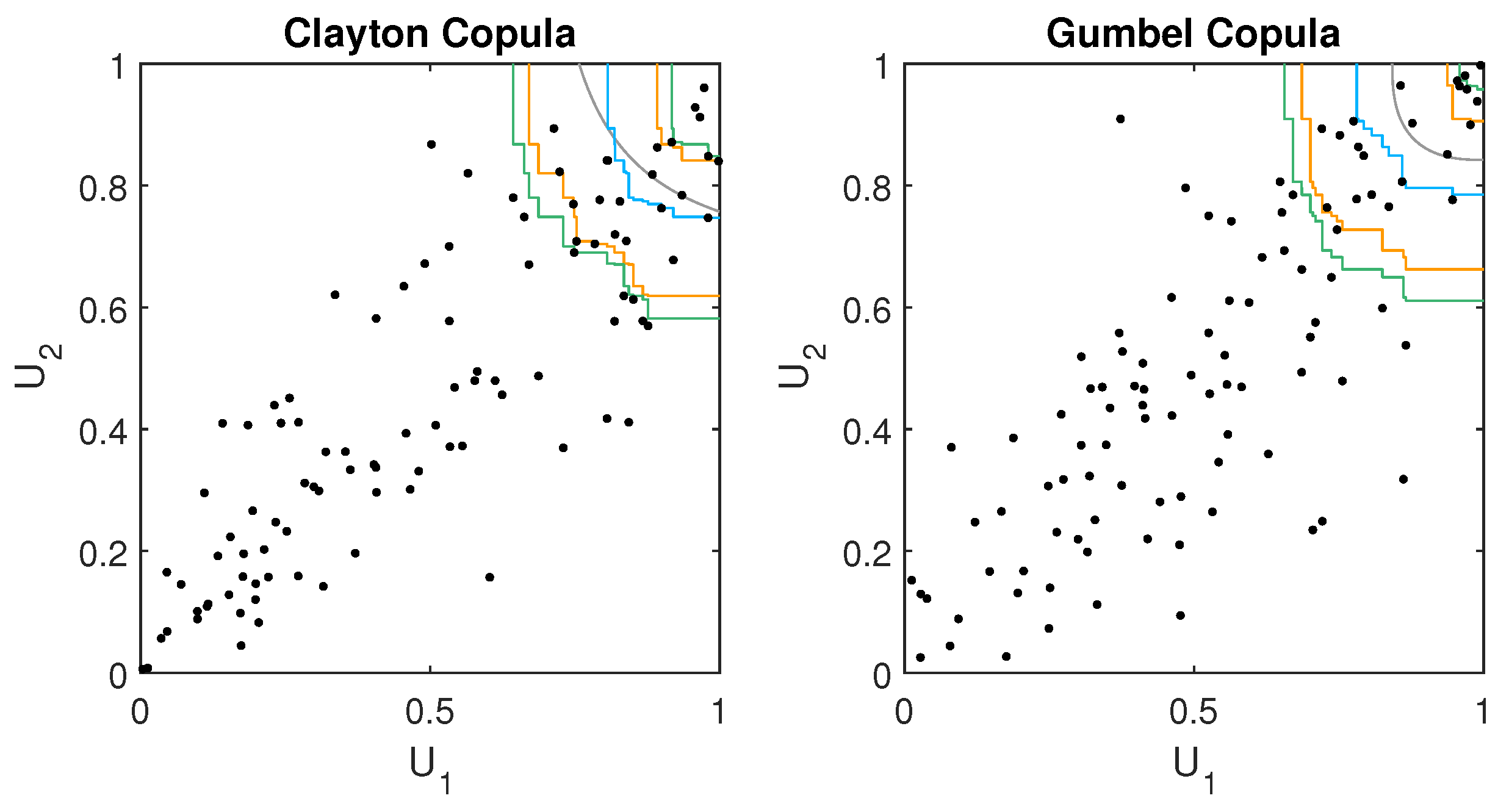
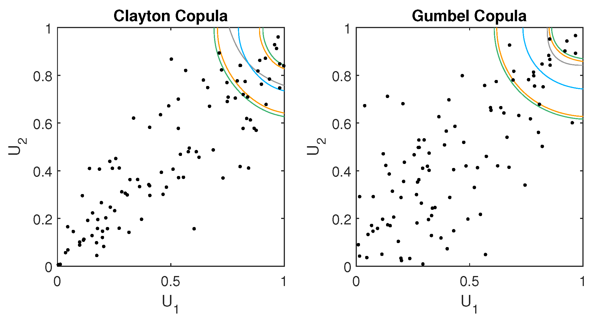
For each setting, we estimate confidence regions for the $p=0.1,0.5,0.9$ multivariate quantile to get a better picture of the performance on the whole copula domain. Confidence regions are estimated at the $90\%$ and $95\%$ confidence levels. For this, we use 1000 bootstraps for the Mammen and Polonik [14] approach and 200 bootstraps for the Chen et al. [15] approach, due to the high computation times of the latter. Each simulation setting is repeated 1000 times to obtain reliable results. The coverage probability is calculated by checking whether the theoretical multivariate quantile boundary lies within the estimated confidence region in each simulation run. For example, Figure 1 and Figure 2 show cases where the theoretical multivariate quantile is covered by the confidence region.

The coverage probabilities for the extended Mammen and Polonik [14] approach can be found in Table 1. The first sanity check which can be made is that the $95\%$ confidence region exhibits higher coverage probabilities than the $90\%$ confidence region, which is the case throughout. Most of the settings for the $10\%$ and $50\%$ multivariate quantiles show more conservative coverage probabilities than the respective confidence level would suggest. In contrast to that, particularly the negative dependence settings for $p=0.9$ exhibit too low coverage probabilities. Too high and too low coverage probabilities could be due to the estimation uncertainty of $K^{-1}$ and the bounded copula domain. The results over the different sample sizes are very similar. We conclude from this that the estimator works quite well for small sample sizes. Overall, the results for the Mammen and Polonik [14] approach are reasonable.

Table 1. Simulation results for the extended Mammen and Polonik [14] approach. The overall coverage probabilities are reasonable.

			$1-\mathit{\alpha }=90\%$						$1-\mathit{\alpha }=95\%$
			$\mathit{n}=\mathbf{100}$			$\mathit{n}=\mathbf{200}$			$\mathit{n}=\mathbf{100}$			$\mathit{n}=\mathbf{200}$
Copula		$\mathit{p}$	$\mathbf{0.1}$	$\mathbf{0.5}$	$\mathbf{0.9}$	$\mathbf{0.1}$	$\mathbf{0.5}$	$\mathbf{0.9}$	$\mathbf{0.1}$	$\mathbf{0.5}$	$\mathbf{0.9}$	$\mathbf{0.1}$	$\mathbf{0.5}$	$\mathbf{0.9}$
	$\mathbf{\tau }$
Gauss	$-0.8$		100	97.7	82.6	100	97.8	80.7	100	99.2	91.9	100	98.8	89.1
	$-0.5$		100	93.3	82.0	100	93.1	84.3	100	96.3	90.8	100	97.2	92.3
	0		99.4	89.6	85.2	99.4	89.8	86.0	99.8	94.4	93.1	100	95.1	93.0
	$0.5$		97.1	92.0	91.3	98.1	89.6	89.6	98.7	96.1	96.1	99.5	94.9	94.7
	$0.8$		96.5	92.7	94.5	96.7	90.6	93.0	98.0	96.6	97.2	98.8	95.5	97.4
Clayton	$0.3$		98.5	91.6	89.6	98.1	91.9	86.4	99.5	96.0	95.2	99.1	95.8	93.8
	$0.5$		97.1	91.1	90.2	97.4	88.9	88.7	98.7	94.9	95.6	98.9	94.2	95.5
	$0.8$		97.2	93.7	92.9	97.2	93.6	92.7	98.2	96.5	96.7	98.4	97.2	97.2
Gumbel	$0.3$		98.5	89.4	88.8	98.3	89.9	87.8	99.7	93.7	95.3	99.7	95.1	94.6
	$0.5$		98.1	91.6	91.7	98.2	89.7	90.3	99.4	96.0	96.6	99.1	94.3	95.4
	$0.8$		96.8	93.1	94.9	96.5	89.9	94.1	98.7	97.1	97.9	98.4	95.2	97.2

The results of the extended Chen et al. [15] approach can be found in Table 2. Most of the coverage probabilities are too low. In particular, confidence regions for high dependence seem to be problematic. In contrast to that, the results are reasonable for low to medium strong dependence, i.e., $\tau \in [-0.5,0.5]$. This could be due to several effects. First, the bounded copula domain could be an issue. Second, the original approach by Chen et al. [15] was developed for densities and not for copulas which are distribution functions. In addition, the estimation of $K_C^{-1}$ is present in the approach. However, we do not think that the latter plays an important role since the results for the Mammen and Polonik [14] approach are good where estimation of $K_C^{-1}$ is also necessary. Finally, we calculate the coverage probabilities by checking whether the level curve at level $K_C^{-1}(p)$ of the underlying copula C is within the boundaries of the constructed confidence set since we are actually interested in the level curves of the copula C. In contrast to that, the approach of Chen et al. [15] aims to estimate confidence regions for the level curves of a convolution of the copula C and the kernel ${\mathbf{K}}_h$, whereby a certain smoothness and limit behavior of the results in ensured. This could lead to the biased coverage probabilities in our case.

Table 2. Simulation results for the extended Chen et al. [15] approach. The overall results are mixed.

			$1-\mathit{\alpha }=90\%$						$1-\mathit{\alpha }=95\%$
			$\mathit{n}=\mathbf{100}$			$\mathit{n}=\mathbf{200}$			$\mathit{n}=\mathbf{100}$			$\mathit{n}=\mathbf{200}$
Copula		$\mathit{p}$	$\mathbf{0.1}$	$\mathbf{0.5}$	$\mathbf{0.9}$	$\mathbf{0.1}$	$\mathbf{0.5}$	$\mathbf{0.9}$	$\mathbf{0.1}$	$\mathbf{0.5}$	$\mathbf{0.9}$	$\mathbf{0.1}$	$\mathbf{0.5}$	$\mathbf{0.9}$
	$\mathit{\tau }$
Gauss	$-0.8$		0.0	0.5	93.0	0.0	0.0	76.8	0.2	2.7	96.8	0.0	0.0	93.2
	$-0.5$		96.1	87.0	93.9	89.2	69.0	93.0	98.1	94.8	96.9	95.4	81.9	97.0
	0		86.1	91.5	94.7	89.2	91.9	93.1	91.5	95.9	97.8	94.3	96.2	97.1
	$0.5$		79.5	83.1	90.0	78.5	80.2	89.6	87.9	90.0	95.9	86.7	86.6	95.6
	$0.8$		71.3	63.0	79.7	62.8	51.7	70.9	80.1	74.6	89.0	74.3	65.5	81.6
Clayton	$0.3$		77.2	87.8	93.4	75.5	84.4	93.3	84.4	93.0	97.4	85.6	91.7	96.7
	$0.5$		69.8	77.5	94.0	65.3	73.4	91.9	79.5	85.0	97.3	76.3	82.9	96.3
	$0.8$		58.1	51.7	87.6	43.8	37.0	87.8	71.0	65.4	94.0	57.7	50.5	92.9
Gumbel	$0.3$		84.7	89.3	91.4	88.4	88.1	90.2	91.0	94.5	96.7	93.5	93.8	95.2
	$0.5$		83.8	82.8	88.3	82.8	80.6	86.4	90.1	90.2	94.7	90.5	89.4	92.9
	$0.8$		74.1	67.6	71.5	67.5	53.8	66.3	84.0	77.4	82.2	77.9	67.3	78.3

In conclusion, the simulation study shows a reasonable performance of the extended Mammen and Polonik [14] method. On the other hand, results for the extended Chen et al. [15] method are mixed. They are, however, reasonably precise for low to medium strong dependence. In summary, we advise practitioners to use the Mammen and Polonik [14] approach for construction of multivariate quantile confidence regions. In the next section, we apply the introduced methods on a small hydrology related data set to gain further insights.

5. Application

We apply the two confidence region approaches on a small data set with a hydrology context. The data can be found in [35]. It comprises 33 yearly maximum values of flood peak and flood volume of the Ashuapmushuan basin in Quebec, Canada. The observations were collected in the period 1963–1995. In a first step, we rank-transform the data to obtain the pseudo observations in the copula domain ${[0,1]}^2$. Figure 3 shows a scatterplot of the original data and the rank-transformed data. The data exhibit positive dependence with a Kendall’s $\tau$ of approximately $0.41$.

Figure 3. Left Panel: 33 flood peak and flood volume observations from the Ashuapmushuan basin in Quebec, Canada. Right Panel: The same data, but rank-transformed to the copula domain ${[0,1]}^2$.

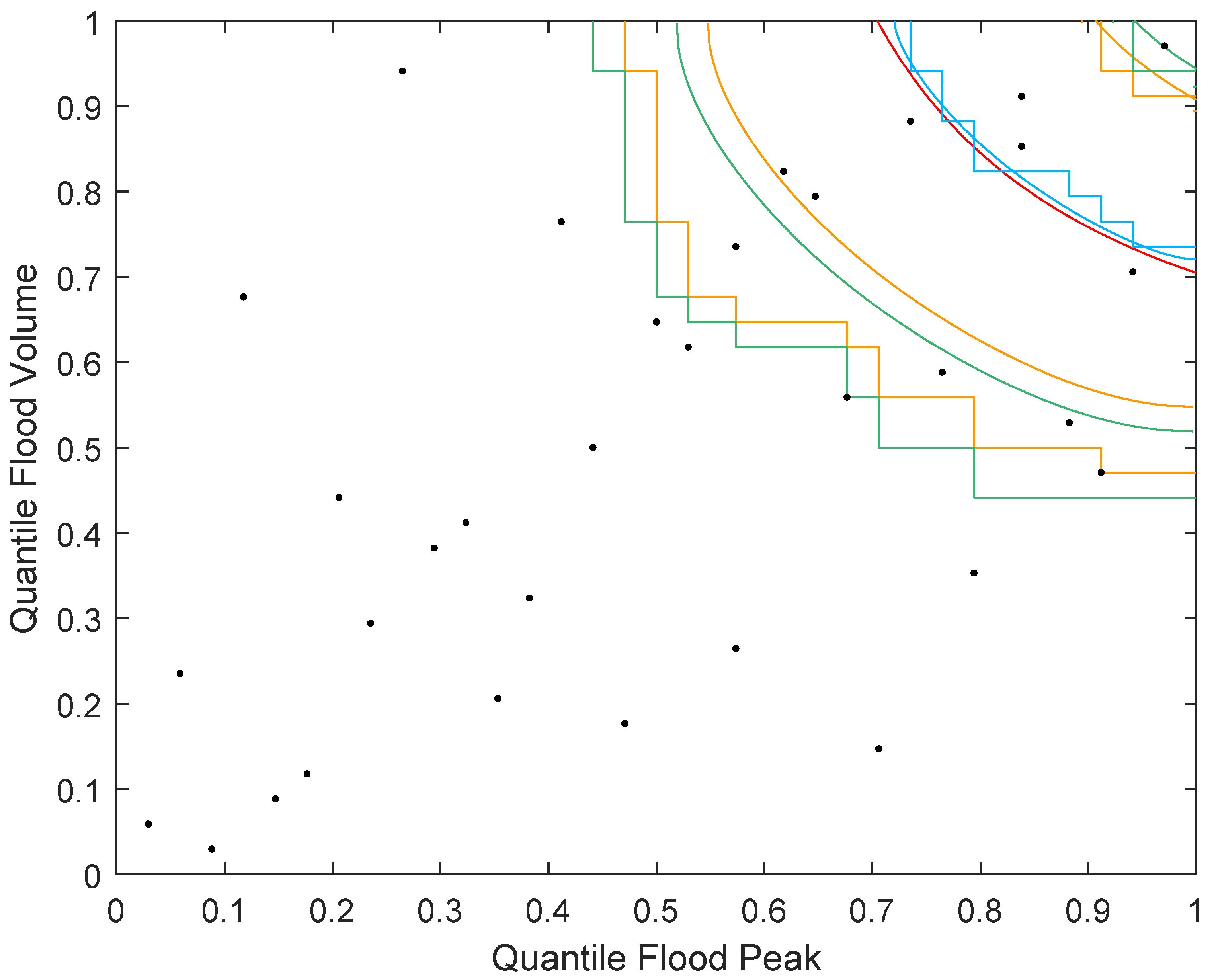
In a second step, we estimate the $90\%$ (i.e., $p=0.9$) multivariate quantile with the two estimators ${\widehat{S}}_p(\widehat{C})$ and ${\widehat{S}}_p({\widehat{C}}_h)$. The estimation results are shown in Figure 4. As can be seen, the two estimated boundaries nicely overlap. For comparison purposes, we additionally estimate a parametric copula model. A Clayton copula with parameter $\theta$ ≈ 1.4 fits the data best among Gumbel, Frank, Gauss-, and t-copulas. The estimated boundary is shown in Figure 4 as a red line and is close to the non-parametric estimates.

Figure 4. Combined estimation results of the multivariate quantile with both confidence region methods. Boundaries of the estimated multivariate quantiles ${\widehat{S}}_p(\widehat{C})$ and ${\widehat{S}}_p({\widehat{C}}_h)$ are shown as a blue step curve and a blue smooth curve, respectively. The red curve refers to the boundary of the multivariate quantile of a Clayton copula that is parametrically estimated on the data. Confidence regions of ${\widehat{S}}_p(\widehat{C})$ for confidence levels $90\%$ and $95\%$ are depicted as orange and green step curves, whereas the confidence regions of ${\widehat{S}}_p({\widehat{C}}_h)$ are shown as orange and green lines for the respective confidence levels.

In a third step, we apply the extended method of Mammen and Polonik [14] as introduced in Section 3.1 to the data. The result of this can be seen in Figure 4. The orange and green step curves depict the confidence region boundaries for confidence levels $90\%$ and $95\%$, respectively. Recall that the boundary of the $90\%$ multivariate quantile partitions the copula domain into a set comprising $10\%$ of the probability mass, which lies to the upper right of the boundary, and a set comprising $90\%$ of the probability mass, which lies to the lower left of the boundary. Counting the points within the confidence region boundaries, we obtain between $33\%$ and $3\%$ of the points for the $90\%$ confidence region and between $36\%$ and $3\%$ of the points for the $95\%$ confidence region. Thus, the confidence regions seem wide, which has to be related to the small sample size though.

Next, we also apply the extended method of Chen et al. [15] as introduced in Section 3.2. Figure 4 shows the results. The orange and green smooth lines depict the confidence region boundaries for confidence levels $90\%$ and $95\%$, respectively. With the same calculations as above, both the $90\%$ confidence region and the $95\%$ confidence region enclose between $21\%$ and $3\%$ of the points. Thus, the confidence regions are tighter than those of the Mammen and Polonik [14] method. This can also be seen in Figure 4. Clearly, the approach of Chen et al. [15] gives a tighter confidence region on the lower end, whereas the two approaches give similar results on the upper end. This has to be put in light of the simulation study, which shows too liberal coverage probabilities for the method of Chen et al. [15] in the considered case $p=0.9$ and moderate positive dependence.

Furthermore, we analyze the secondary return period as defined in [36]. The estimated secondary return period given by the multivariate quantile is $\frac{1}{1-{\widehat{K}}_C(P)}=10$ years. For the Mammen and Polonik [14] approach, the confidence regions suggest a secondary return period between 3 and 33 years and between $2.75$ and 33 years for the $90\%$ and $95\%$ confidence levels, respectively. The confidence regions of the Chen et al. [15] approach suggest a secondary return period between $4.7$ and 33 years and between $4.1$ and 33 years for the $90\%$ and $95\%$ confidence levels, respectively. Thus, the confidence regions can also be used to assess the precision of the implied secondary return period of the multivariate quantile.

Finally, we want to stress again the advantages of having confidence regions for multivariate quantiles in a hydrology context. Not only do confidence regions give a statistical insight into the estimation uncertainty present, e.g., Figure 4 shows that these are very wide and more data would be needed for a reliable estimate of the multivariate quantile, but they are also helpful to the design of infrastructures. Since the true multivariate quantile boundary lies within the confidence region boundaries at the specified confidence level, the points within the confidence region should be considered when planning, e.g., new dams. In particular, a point from within the region between the lower boundary of the confidence region and the multivariate quantile boundary could actually be a point with a (true) secondary return period of 10 years and thus would be rarer than the estimated multivariate quantile suggests. Conversely, a point from within the region between the upper boundary of the confidence regions and the multivariate quantile boundary could have a lower (true) secondary return period and thus would occur more often than might be expected from considering the estimated multivariate quantile boundary only.

6. Conclusions

We extend the two approaches by Mammen and Polonik [14] and Chen et al. [15] for construction of confidence regions for level sets to make them applicable in a multivariate quantile context. This involves incorporating the estimation of the quantile level via the inverse Kendall distribution function $K_C^{-1}$ and also adjusting for the bounded copula domain. Accompanying MATLAB code can be found in the Supplementary Material.

The simulation study shows reasonable coverage probabilities for the extended Mammen and Polonik [14] method. Some of the coverage probabilities are too conservative. However, in particular for negative dependence and high quantile levels, the approach yields too low coverage probabilities. On the other hand, the extended Chen et al. [15] method shows mixed results. Overall, the coverage probabilities are too liberal. However, they show a reasonable precision for low to medium strong dependence. An application on a small hydrology-related data set illustrated some further aspects of the approaches.

On a final note, we want to point out that we tried to keep the extension of the methods as simple as possible. The approaches could be extended in several further ways. For example, a smoothed bootstrap along the lines of [10] can be incorporated into the analysis. However, we will leave this for future research. We hope that practitioners in hydrology and other fields find the considered approaches helpful and easy to apply to their problems at hand.

References

- Yue, S.; Rasmussen, P. Bivariate frequency analysis: Discussion of some useful concepts in hydrological application. Hydrol. Process. 2002, 16, 2881–2898. [Google Scholar] [CrossRef]
- Salvadori, G. Bivariate return periods via 2-Copulas. Stat. Methodol. 2004, 1, 129–144. [Google Scholar] [CrossRef]
- Salvadori, G.; De Michele, C. Frequency analysis via copulas: Theoretical aspects and applications to hydrological events. Water Resour. Res. 2004, 40, 1–17. [Google Scholar] [CrossRef]
- Chebana, F.; Ouarda, T. Multivariate quantiles in hydrological frequency analysis. Environmetrics 2011, 22, 63–78. [Google Scholar] [CrossRef]
- Salvadori, G.; Tomasicchio, G.R.; D’Alessandro, F. Practical guidelines for multivariate analysis and design in coastal and off-shore engineering. Coast. Eng. 2014, 88, 1–14. [Google Scholar] [CrossRef]
- Salvadori, G.; Durante, F.; Tomasicchio, G.R.; D’Alessandro, F. Practical guidelines for the multivariate assessment of the structural risk in coastal and off-shore engineering. Coast. Eng. 2015, 95, 77–83. [Google Scholar] [CrossRef]
- Salvadori, G.; Durante, F.; De Michele, C.; Bernardi, M.; Petrella, L. A multivariate copula-based framework for dealing with hazard scenarios and failure probabilities. Water Resour. Res. 2016, 52, 3701–3721. [Google Scholar] [CrossRef]
- Salvadori, G.; De Michele, C. On the Use of Copulas in Hydrology: Theory and Practice. J. Hydrol. Eng. 2007, 12, 369–380. [Google Scholar] [CrossRef]
- Salvadori, G.; Durante, F.; Perrone, E. Semi-parametric approximation of Kendall’s distribution function and multivariate Return. J. Soc. Fr. Stat. 2013, 154, 151–173. [Google Scholar]
- Coblenz, M.; Dyckerhoff, R.; Grothe, O. Nonparametric estimation of multivariate quantiles. Environmetrics 2018, 29, e2488. [Google Scholar] [CrossRef]
- Serinaldi, F. An uncertain journey around the tails of multivariate hydrological distributions. Water Resour. Res. 2013, 49, 6527–6547. [Google Scholar] [CrossRef]
- Serinaldi, F. Can we tell more than we can know? The limits of bivariate drought analyses in the United States. Stoch. Environ. Res. Risk Assess. 2016, 30, 1691–1704. [Google Scholar] [CrossRef]
- Hyndman, R.J. Computing and Graphing Highest Density Regions. Am. Stat. 1996, 50, 120–126. [Google Scholar]
- Mammen, E.; Polonik, W. Confidence regions for level sets. J. Multivar. Anal. 2013, 122, 202–214. [Google Scholar] [CrossRef]
- Chen, Y.C.; Genovese, C.R.; Wasserman, L. Density Level Sets: Asymptotics, Inference, and Visualization. J. Am. Stat. Assoc. 2017, 112, 1684–1696. [Google Scholar] [CrossRef]
- Sklar, A. Fonctions de répartition à n dimensions et leurs marges. Publ. Inst. Stat. Univ. Paris 1959, 8, 229–231. [Google Scholar]
- Nelsen, R.B. An Introduction to Copulas; Springer Series in Statistics; Springer: New York, NY, USA, 2006. [Google Scholar]
- Joe, H. Dependence Modeling with Copulas; Chapman & Hall: Boca Raton, FL, USA, 2015. [Google Scholar]
- Durante, F.; Sempi, C. Principles of Copula Theory; CRC/Chapman & Hall: Boca Raton, FL, USA, 2016. [Google Scholar]
- Genest, C.; Favre, A.-C. Everything You Always Wanted to Know about Copula Modeling but Were Afraid to Ask. J. Hydrol. Eng. 2007, 12, 347–368. [Google Scholar] [CrossRef]
- Omelka, M.; Gijbels, I.; Veraverbeke, N. Improved kernel estimation of copulas: Weak convergence and goodness-of-fit testing. Ann. Stat. 2009, 37, 3023–3058. [Google Scholar] [CrossRef]
- Silverman, B.W. Density Estimation for Statistics and Data Analysis; Chapman & Hall: London, UK, 1986. [Google Scholar]
- Barbe, P.; Genest, C.; Ghoudi, K.; Remillard, B. On Kendall’s Process. J. Multivar. Anal. 1996, 58, 197–229. [Google Scholar] [CrossRef]
- Genest, C.; Rivest, L.-P. On the multivariate probability integral transform. Stat. Prob. Lett. 2001, 53, 391–399. [Google Scholar] [CrossRef]
- Nelsen, R.B.; Quesada-Molina, J.J.; Rodríguez-Lallena, J.A.; Úbeda-Flores, M. Kendall distribution functions. Stat. Prob. Lett. 2003, 65, 263–268. [Google Scholar] [CrossRef]
- Serfling, R. Approximation Theorems of Mathematical Statistics; John Wiley & Sons: Hoboken, NJ, USA, 1980. [Google Scholar]
- Ghoudi, K.; Rémillard, B. Empirical processes based on pseudo-observations. In Asymptotic Methods in Probability and Statistics, A Volume in Honour of Miklós Csörgö; Szyskowicz, B., Ed.; Elsevier: New York, NY, USA, 1998; pp. 171–197. [Google Scholar]
- Coblenz, M.; Grothe, O.; Schreyer, M.; Trutschnig, W. On the length of copula level curves. J. Multivar. Anal. 2018, 167, 347–365. [Google Scholar] [CrossRef]
- Tibiletti, L. On a new notion of multidimensional quantile. Metron 1993, 51, 77–83. [Google Scholar]
- Chaudhuri, P. On a Geometric Notion of Quantiles for Multivariate Data. J. Am. Stat. Assoc. 1996, 91, 862–872. [Google Scholar] [CrossRef]
- Serfling, R. Quantile functions for multivariate analysis: Approaches and applications. Stat. Neerl. 2002, 56, 214–232. [Google Scholar] [CrossRef]
- Di Bernardino, E.; Laloë, T.; Maume-Deschamps, V.; Prieur, C. Plug-in estimation of level sets in a non-compact setting with applications in multivariate risk theory. ESAIM Prob. Stat. 2013, 17, 236–256. [Google Scholar] [CrossRef]
- Deheuvels, P. La fonction de dépendance empirique et ses propriétés. un test non paramétrique d’indépendance. Académie Royale de Belgique. Bulletin de la Classe des Sciences 1979, 65, 274–292. [Google Scholar]
- Deheuvels, P. Nonparametric test of independence. In Statistique non Paramétrique Asymptotique; Lecture Notes in Mathematics; Raoult, J.-P., Ed.; Springer: Berlin, Germany, 1980; Volume 821, pp. 95–107. [Google Scholar]
- Yue, S.; Ouarda, T.; Bobée, B.; Legendre, P.; Bruneau, P. The Gumbel mixed model for flood frequency analysis. J. Hydrol. 1999, 226, 88–100. [Google Scholar] [CrossRef]
- Salvadori, G.; De Michele, C.; Durante, F. On the return period and design in a multivariate framework. Hydrol. Earth Syst. Sci. 2011, 88, 1–14. [Google Scholar] [CrossRef]
© 2018 by the authors. Licensee MDPI, Basel, Switzerland. This article is an open access article distributed under the terms and conditions of the Creative Commons Attribution (CC BY) license (http://creativecommons.org/licenses/by/4.0/).