Abstract
Precipitation is the main input in the water balance of watersheds; therefore, correct estimates are necessary for water resources management and decision making. In south-central Chile there is a low density of precipitation gauges (~1 station/675 km2), most of which are located in low-altitude areas. The spatial distribution of precipitation is, therefore, not properly recorded. In this study an inverse modeling approach is used to estimate the extent to which precipitation amounts must be corrected. Using a lumped water balance model, a factor for correcting precipitation data is calculated for 41 watersheds located in south-central Chile. Then, based on a geo-statistical interpolation, a map for correcting the precipitation amounts is proposed and a validation of these corrections is achieved. The results show that in gently sloping areas, the precipitation records are more representative than in steep mountain areas. In addition, the higher the mountains, the less representative the precipitation records become.
1. Introduction
The climate is important as a regulating factor of the natural and human environment on both the population level and in terms of daily activities. In this regard, precipitation is among the climatic elements that most influence nature and its configuration [1]. Its temporal and spatial distribution determine cycles in agriculture and forestry, which are the main economic activities of south-central Chile, where both productivity and the development of the primary plant and animal species depend on water resources from mountainous areas.
Having an accurate understanding of the availability of water resources has become important and necessary. This variable depends to a large extent on the storage and regulation capacities of mountain watersheds and the climate variability that affects the area [2]. The precipitation regime in south-central Chile (lat. 34°–40° S) is associated mainly with the successive passage of frontal systems resulting from the seasonal shift of the South Pacific subtropical anticyclone (April to September) [3], which enter the continent from the Pacific Ocean. During warmer months, meanwhile, the anticyclone shifts a few degrees to the south, impeding the formation of precipitation associated with the passage of such frontal systems.
The Coastal and Andes mountain ranges generate strong precipitation gradients that can also vary among storms, locally modifying precipitation amounts recorded by precipitation gauge stations [4]. However, due to its low density, the precipitation gauge station network in Chile may prove insufficient for correctly characterizing spatial precipitation variability. For example, in south-central Chile, there is a precipitation gauge station density of approximately 1 precipitation gauge every 675 km2, and most of these stations are concentrated in the Central Valley and along the coast. This density is very low in comparison to the recommendations of the World Meteorological Organization (WMO); according to the WMO [5], to have a good precipitation gauge network in terms of density, there must be at least one precipitation gauge every 250 km2 in mountainous areas and one every 575 km2 in interior plains [5,6]. In addition, the presence of mountainous reliefs complicates access and impedes the installation of precipitation gauge stations; therefore, there is a much lower density in areas such as the western slope of the Andes and the highlands of the Coastal Range (e.g., Nahuelbuta Range, lat. ~37°45′ S). Thus, in a watershed with areas that are mostly mountainous, precipitation may be underestimated since the increase in precipitation due to the orography may not correctly represented.
Precipitation variability in both spatial and temporal terms is influenced by atmospheric thermodynamics, which depend on topography and relief, introducing marked imbalances in the spatial distribution of precipitation [7]. Daly et al. [8] hold that the main source of uncertainty in the characterization of the spatial distribution of precipitation is related to mountain height and meteorological factors such as atmospheric stability and moisture availability, among others. Therefore, it proves necessary to estimate precipitation in watersheds with a complex topography such as those of south-central Chile—with the presence of the Coastal Range and the Andes—for appropriate hydrological management.
There are numerous simulation models in the literature that can be applied to determine total watershed input [2,9,10,11,12,13]. Water availability in a watershed can be quantified through hydrological models; however, in order to achieve this objective, it is necessary to compile information on its meteorology, streamflows and geomorphology. The objective of this study is to quantify the effect of the morphology of south-central Chile (Coastal Range–Central Valley–Andes) on the spatial distribution of precipitation and its relationship to annual precipitation records from the national precipitation gauge network in order to propose a correction alternative for the available records. To this end, a spatially distributed precipitation correction factor was determined through inverse modeling, allowing recorded precipitation amounts to be related to precipitation increases, comparing the net input and output volumes per watershed in south-central Chile.
2. Study Area
The study area includes 41 watersheds located in south-central Chile (lat. ~34.5° to 39.5° S, Figure 1). Of these, 15 are located in the Andes, 16 in the Central Valley, and 10 in the Coastal Range.
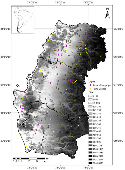
Figure 1.
Study area, with locations of precipitation gauge stations (circles) and streamflow gauging stations (rhombuses). Made by the authors.
The study area is ~100,000 km2 and includes the Coastal Range (with an average elevation of 1200 m.a.s.l.), the Andes (with altitudes greater than 4000 m.a.s.l.) and the Central Valley. This last area is a flat valley located between the two mountain ranges (see topography in Figure 1). The area has an average precipitation gauge density of 1 precipitation gauge every 675 km2, which can be subdivided into 1 precipitation gauge every 540 km2 in low zones (below 400 m.a.s.l.) and 1 precipitation gauge every 960 km2 in mountainous areas (above 400 m.a.s.l.). In mountainous areas, the station density is a quarter of that recommended by the World Meteorological Organization [5].
3. Data
To carry out the study, an inverse hydrological modeling approach was used, which consists of deriving the precipitation inputs to a watershed from modeling and comparing the results of a model with streamflow records in the modeled watershed.
The modeling requires monthly series of precipitation, streamflow, air temperature and potential evapotranspiration values, in addition to the morphological characterization of each watershed, which was constructed with a digital terrain model made from 1-arc-second-resolution (30 m) ASTER (Advanced Spaceborne Thermal Emission and Reflection Radiometer) images.
Regarding the input data, monthly precipitation time series were collected from precipitation gauge stations managed by the National Water Directorate (Dirección General de Aguas, DGA) (see Figure 1). The inverse distance weighting (IDW) method was used to calculate the representative precipitation of each watershed. With respect to temperature records, there were no stations with continuous monthly series and the spatial distribution required for this study; therefore, monthly temperature series provided by University of Delaware (UD) Center for Climatic Research were used [14]. To estimate potential evapotranspiration (PE), the formula proposed by Thornthwaite [15] and UD temperature data series were used. The spatial distribution of these variables over each watershed was determined using Thiessen polygons. Regarding streamflows, monthly series were collected from streamflow gauging stations managed by the DGA, as indicated in Figure 1.
Due to the availability and quality of the input data, the analysis was carried out at a monthly time step over a minimum time window of 10 years.
4. Methods
4.1. Conceptual Model Description
The model used in this article is the conceptual water balance model presented in Muñoz [16] and Muñoz et al. [13] (Figure 2). The model simulates the precipitation-runoff and snowmelt-runoff processes separately. Because the pluvial regime predominates in the study area, only the precipitation-runoff module was used in this study, and it will be briefly described here.
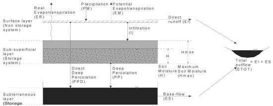
Figure 2.
Conceptual model diagram. Made by the authors.
The lumped model considers the watershed a double storage system consisting of subsurface (SS) and deep storage (US). SS represents the water stored in the unsaturated soil layer as soil moisture, while US is the water covering the saturated soil layer. The main input data for the model are precipitation (PM) and potential evapotranspiration (PET). The model output is the total runoff (ETOT) at the watershed outlet, which includes both base flow (ES) and surface runoff (EI). For a further description of the model’s characteristics, please refer to Muñoz [16] and Muñoz et al. [13]. In addition, Table 1 presents a brief description of the model parameters and their influence on the model.

Table 1.
Description of the model parameters, adjustment factors, and conceptual-physical range for the precipitation-runoff model.
4.2. Calibration and Calculation of the Precipitation Correction Factor
To calibrate the models implemented in each watershed, the Monte Carlo Analysis Toolbox (MCAT) and the identifiability analysis developed by Wagener and Kollat [17] were used. This analysis allows the estimation of a set of suitable parameters in order to obtain good-performing models [18] based on a predefined performance measure or objective function. To assess identifiability, MCAT operates by running repeated simulations with a randomly selected parameter set within a user-defined range. This range must be wide enough to cover any possible simulation combination and at the same time must be a valid conceptual range for the purposes of the modeling. Then, the parameter values are compared with the values obtained for the objective function for subsequent analyses.
The identifiability analysis consists of a graphic representation of a sensitivity analysis applied to the best 10% of the simulations and allows parameter ranges and processes that positively influence the model outputs (with respect to a given objective function) to be found, and thereby helps restrict the parameter range such that only good-performing models are kept [19,20]. In addition, it allows the uncertainty associated with predictions to be determined and reduced, improving the quality of the hydrological model and the reliability of the outputs [13].
In the present study, 10,000 simulations were carried out for each model (watershed), and the precipitation adjustment factor (A) was calculated by taking the 50th percentile (P50) of the best 10% of the models according to the identifiability analysis and three objective functions. The root mean square error (RMSE), transformed root mean square error (TRMSE) and the runoff coefficient error (ROCE) functions, designed to calibrate a model as a function of high streamflows, low streamflows and long-term water balance closure, respectively, were used [21].
To ensure process and simulated-flow representativeness, it was verified that only behavioral models were considered within the best 10% models. Nash–Sutcliffe values higher than 0.6 were used as an acceptance criterion for behavioral models.
4.3. Objective Function Description
- (i)
- Root mean square error (RMSE) (Equation (1)): this indicator operates as a function of simple differentials of the simulated streamflows (Qs,t) with respect to the observed streamflows (Qo,t) and is focused on the high flows.
- (ii)
- Transformed root mean square error (TRMSE) (Equations (2) and (3)): this function is equivalent to RMSE, with the difference that the simulated and observed values are first transformed through Box–Cox transformation, which results in low flows taking on greater importance than medium or high flows.
- (iii)
- Runoff coefficient error (ROCE) (Equation (4)): this indicator captures the overall water balance, as it combines the flows into just one descriptor of hydrological characteristics—the average annual runoff coefficient—defined as (). The differences in absolute value between the simulated and observed descriptors are compared. This descriptor calculates the volumetric differences between simulated and observed streamflows over a modeling period, and therefore is the most suitable function for the objective of this study.
5. Results
Table 2 shows the results obtained from the identifiability analysis (P50 of the best 10% of the models, of a total of 10,000 simulations) of factor A. As a complement, Table 2 shows: (i) average annual precipitation calculated for each watershed from DGA records using the inverse distance weighting method to estimate the representative precipitation of each watershed (AAPP); (ii) average annual precipitation calculated from average annual precipitation isohyets from the national water balance made by the DGA [22] (AAPI); and (iii) average annual precipitation (AAP) calculated from inverse modeling using three objective functions (AAPRMSE, AAPTRMSE and AAPROCE).

Table 2.
Precipitation correction factors estimated by inverse modeling for each watershed, using three objective functions. In addition, the average annual precipitation amounts from National Water Directorate (DGA) precipitation gauge records (AAPP), isohyets (AAPI) and inverse modeling (AAPc) using different objective functions are shown. Made by the authors.
Taking the AAPP values as a reference point for the precipitation of each watershed, the percent difference in the AAP was calculated from isohyets and inverse modeling. Thus, the greater the difference in absolute value, the less representative the recorded precipitation is of the precipitation in the watershed, while positive differences suggest an underestimation of AAPP values and negative differences an overestimation. Consolidated results are shown in box plots grouped by watershed location (Andes, Central Valley and Coastal Range) (Figure 3).
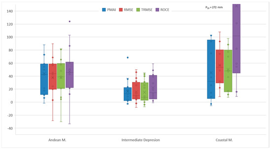
Figure 3.
Percent difference in the AAP calculated by isohyets and inverse modeling for each watershed. Made by the authors.
Figure 3 shows that, in general, precipitation tends to be underestimated, although the differences are smaller in areas with flatter topography such as the Central Valley [23]. In addition, in the Andes these differences increase, probably because the increase in precipitation due to the orographic effect caused by the Andes is not properly measured by the existing stations [24]. This effect is also observed in the Coastal Range, although it is most noticeable in areas where the cordillera is higher (e.g., Nahuelbuta Range, lat. ~37°45′ S) [25]. Similar results have been obtained in hydrological studies and watershed-scale precipitation analysis in various watersheds in south-central Chile (e.g., [13,23,24,25,26,27,28]). In general, it is concluded that precipitation in cordillera zones is underestimated by between 20% and 90%.
As the model is a lumped water balance model, all the values considered in the modeling stage are assumed to be uniformly distributed in a watershed. Therefore, a point value at the geometric center of each watershed was considered representative of the precipitation and correction factor of each modeled watershed. To consolidate the results a cokriging-z (with ground elevation as auxiliary variable), geospatial interpolation of AAPROCE (Figure 4a) and the precipitation correction factor estimated using the ROCE function (AROCE, Figure 4b) was carried out. AAPROCE and AROCE values were assumed to be at the geometric center of each modeled watershed. Figure 4 leads to the same conclusions as those obtained from Figure 3. On the map it is observed that the area with the closest calculated and measured precipitation values is the Central Valley, where factor A varies around 1.
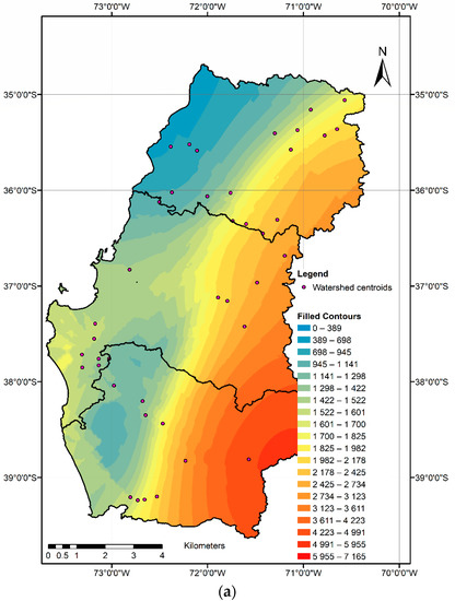
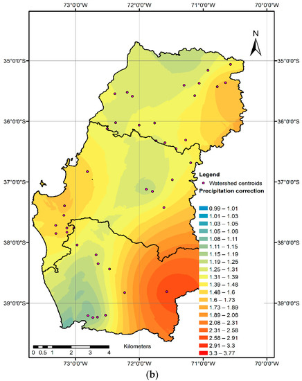
Figure 4.
(a) Estimated average annual precipitation based on the results of inverse modeling and a cokriging-z interpolation; (b) Spatially distributed factor for precipitation correction using an approximation of the inverse model and a cokriging-z interpolation. Made by the authors.
The Central Valley is the sub-area with the least spatial topographic variability and smoothest relief and, therefore, there is not high variability in precipitation caused by the interaction of frontal systems and the topography. This area is also the most accessible and thus has the greatest precipitation gauge station density (1 station every 540 km2) [23]. In addition, in the Andes and Coastal Range there is a strong interaction between the entry of frontal systems and the topography, producing an increase in precipitation as land elevation increases [26,29,30]. This variability, along with the low station density (1 station every 960 km2) explains the underestimation in the calculated precipitation amounts.
The map in Figure 4 allows the extent to which precipitation is underestimated to be seen and provides a useful tool for the correction and estimation of precipitation in south-central Chile. Along with the map, average annual precipitation isohyets every 100 mm were created (not shown in this article) for use in scientific and practical applications. The results of this study in shape file format are included with this manuscript as Supplementary Materials.
6. Conclusions
There is a low precipitation gauge station density in south-central Chile, which varies according to accessibility and is highest in the Central Valley and lowest in the mountainous areas. This density also decreases as mountain height increases, mainly due to decreasing accessibility. Although the density is lower than desired and below the level recommended by the World Meteorological Organization, the estimation and spatial representation of precipitation in the Central Valley proves to be acceptable.
In mountainous areas there is a conspicuous underestimation of precipitation due to the low precipitation gauge density. This underestimation increases along with mountain height, making it necessary to carry out precipitation corrections of up to 3 times the values recorded in the lowest areas.
Correction factors for the precipitation records from the national precipitation gauge network were determined and precipitation correction maps, along with average annual precipitation isohyets corrected for the orography, were made.
It is important to point out that this paper is focused on correcting precipitation records based on observations. It is an attempt to improve the current data availability and knowledge in the study area. Orography may not be the only variable related to spatial variability in the study area, and climate change trends and climate variability are not directly considered in the corrected precipitation amounts. Therefore, caution is necessary if climate projections, hydrological projections, or processes analysis are pursued. Including such signals or components may be necessary for medium- and long-term projections.
Although the hydrological model and its parameters, among other factors, may contribute as sources of uncertainty in the study, we deem the model not necessarily to be a major source, especially in the study area. The results show that precipitation is underestimated by up to 3.7 times in some areas. Therefore, precipitation is a great source of uncertainty for modeling and performing precipitation-related studies. In addition, it is important to point out that the methods include the simple inverse distance weighting method in the experimental design; therefore, corrected precipitation represents a further step in the precipitation estimation of the watersheds.
Supplementary Materials
The 100-mm corrected isohyets generated in this study are available online at http://www.mdpi.com/2073-4441/10/8/1092/s1.
Author Contributions
E.M. designed the experiment, analyses and methods and wrote the paper; M.A., J.L. and I.R. performed the analyses and calculations.
Funding
This research has been supported by the FONDECYT 11121287 project.
Acknowledgments
The authors thank the General Water Directorate (DGA) of the Chilean Ministry of Public Works for providing the precipitation records used in this study and Fondecyt project 11121287, “Hydrological process dynamics in Andean basins. Identifying the driving forces, and implications in model predictability and climate change impact studies”.
Conflicts of Interest
The authors declare no conflict of interest.
References
- Pizarro, R.; Ramírez, C.; Flores, J. Análisis comparativo de cinco métodos para la estimación de precipitación areales anuales en períodos extremos. Bosque 2003, 24, 31–38. [Google Scholar] [CrossRef]
- Zúñiga, R.; Muñoz, E.; Arumí, J.L. Estudio de los Procesos Hidrológicos de la cuenca del Rio Diguillín. Obras Proy. 2012, 11, 69–78. [Google Scholar] [CrossRef]
- Garreaud, R. Comportamiento Atmosférico Asociado a Grandes Crecidas Hidrológicas de Chile Central. Master’s Thesis, Departamento de Geofísica, Universidad de Chile, Santiago, Chile, 1993; p. 133. [Google Scholar]
- Falvey, M.; Garreaud, R. Moisture variability over the South American Altiplano during the SALLJEX observing season. J. Geophys. Res. 2005, 110, D22105. [Google Scholar] [CrossRef]
- WMO–World Meteorological Organization. Guide to Hydrological Practices. Volume I: Hydrology—From Measurement to Hydrological Information, 6th ed.; WMO: Geneva, Switzerland, 2008. [Google Scholar]
- Pizarro, R. Elementos Técnicos de Hidrología III. Proyecto Regional Mayor Sobre Uso y Conservación de Recursos Hídricos en Áreas Rurales de América Latina y el Caribe; Universidad de Talca: Talca, Chile, 1993; p. 135. [Google Scholar]
- Fernandez, F. Manual de Climatología Aplicada. Clima, Medio Ambiente y Planificación; Síntesis: Madrid, Spain, 1995; ISBN 84-7738-275-1. [Google Scholar]
- Daly, C.; Neilson, R.P.; Phillips, D.L. A Statistical Topographic Model for Mapping Climatological Precipitation over Mountainous Terrain. J. Appl. Meteorol. 1994, 33, 140–158. [Google Scholar] [CrossRef]
- Ferrer, P.; Brown, E.; Ayala, L. Simulación de Gastos Mensuales en una Cuenca Pluvial. II Coloquio Nacional de la Sociedad Chilena de Ingeniería Hidráulica; Universidad Católica de Chile: Santiago, Chile, 1973. [Google Scholar]
- Pizarro, R. Análisis Comparativo de Modelos Matemáticos Precipitación-Escorrentía en Cuencas de España Peninsular. Departamento de Ingeniería Forestal, Escuela Técnica Superior de Ingenieros de Montes; Universidad Politécnica de Madrid: Madrid, Spain, 1996; p. 320. [Google Scholar]
- Daly, C.; Smith, J.W.; Smith, J.I.; Mckane, R.B. Highresolution spatial modeling of daily weather elements for a catchment in the Oregon Cascade Mountains, United States. J. Appl. Meteorol. Climatol. 2007, 46, 1565–1586. [Google Scholar] [CrossRef]
- Caro, M.; Rojas, E. Aplicación de Modelación Superficial en Cuencas Pluviales de las Regiones del Maule, Biobío y la Araucanía; Ministerio de Obras Públicas, Dirección General de Aguas, División de Estudios y Planificación: Santiago, Chile, 2010. [Google Scholar]
- Muñoz, E.; Rivera, D.; Vergara, F.; Tume, P.; Arumí, J.L. Identifiability analysis: Towards constrained equifinality and reduced uncertainty in a conceptual model. Hydrol. Sci. J. 2014, 59, 1690–1703. [Google Scholar] [CrossRef]
- Willmott, C.J.; Matsuura, K. Terrestrial Air Temperature and Precipitation: Monthly and Annual Time Series (1900–2014) (V 4.01); University of Delaware: Newark, DE, USA, 2015. [Google Scholar]
- Thornthwaite, C. An approach toward a rational classification of climate. Geogr. Rev. 1948, 38, 55–94. [Google Scholar] [CrossRef]
- Muñoz, E. Desarrollo de un Modelo Hidrológico Como Herramienta de Apoyo para la Gestión del agua. Aplicación a la Cuenca del rio Laja, Chile. Master’s Thesis, Departamento de Ciencias y Técnicas del Agua y del Medio Ambiente, Universidad de Cantabria, Santander, Spain, 2010. [Google Scholar]
- Wagener, T.; Kollat, J. Numerical and visual evaluation of hydrological and environmental models using the Monte Carlo analysis Toolbox. Environ. Model. Softw. 2007, 22, 1021–1033. [Google Scholar] [CrossRef]
- Wagener, T. Evaluation of Catchment models. Hydrol. Process. 2003, 17, 3375–3378. [Google Scholar] [CrossRef]
- Wagener, T.; Gupta, H. Model identification for hydrological forecasting under uncertainty. Stoch. Environ. Res. Risk Assess. 2005, 19, 378–387. [Google Scholar] [CrossRef]
- Gupta, H.V.; Beven, K.; Wagener, T. Model Calibration and Uncertainty Estimation—Encyclopedia of Hydrological Sciences; Anderson; John Wiley & Sons: Hoboken, NJ, USA, 2006. [Google Scholar] [CrossRef]
- Van Werkhoven, K.; Wagener, T.; Reed, P.; Tang, Y. Sensitivity-guided reduction of parametric dimensionality for multi-objetive calibration of watershed models. Adv. Water Resour. 2009, 32, 1154–1169. [Google Scholar] [CrossRef]
- DGA—Dirección General de Aguas. Balance Hídrico de Chile; Ministerio de Obras Públicas: Santiago, Chile, 1987. [Google Scholar]
- Lucero, P. Corrección de la Precipitación Mediante la Aplicación de Modelación Inversa en las Cuencas del Valle Central de Chile; Universidad Católica de la Santísima Concepción: Concepción, Chile, 2015. [Google Scholar]
- Acuña, M. Corrección de la Precipitación Mediante Modelación Inversa en las Cuencas de la Cordillera de los Andes. Ph.D. Thesis, Universidad Católica de la Santísima Concepción, Concepción, Chile, 2015. [Google Scholar]
- Rojas, I. Corrección de la Precipitación por Orografía Mediante Modelación Inversa en Cuencas de la Cordillera de la Costa; Universidad Católica de la Santísima Concepción: Concepción, Chile, 2017. [Google Scholar]
- Castro, L.M.; Gironas, J.; Fernandez, B. Spatial estimation of daily precipitation in regions with complex relief and scarce data using terrain orientation. J. Hidrol. 2014, 517, 481–492. [Google Scholar] [CrossRef]
- Toledo, C.; Muñoz, E.; Zambrano-Bigiarini, M. Comparison of Stationary and Dynamic Conceptual Models in a Mountainous and Data—Sparse Catchment in South-Central Chilean Andes. Adv. Meteorol. 2015, 2015, 526158. [Google Scholar] [CrossRef]
- Muñoz, E.; Arumí, J.L.; Wagener, T.; Oyarzún, R.; Parra, V. Unraveling complex hydrogeological processes in Andean basins in south-central Chile: An integrated assessment to understand hydrological dissimilarity. Hydrol. Process. 2016, 30, 4897–5070. [Google Scholar] [CrossRef]
- Garreaud, R. The Andes climate and weather. Adv. Geosci. 2009, 22, 3–11. [Google Scholar] [CrossRef]
- Falvey, M.; Garreaud, R. Wintertime precipitation episodes in central Chile: Associated meteorological conditions and orographic influences. J. Hydrometeorol. 2007, 8, 171–193. [Google Scholar] [CrossRef]
© 2018 by the authors. Licensee MDPI, Basel, Switzerland. This article is an open access article distributed under the terms and conditions of the Creative Commons Attribution (CC BY) license (http://creativecommons.org/licenses/by/4.0/).