Vulnerability Assessment to Trihalomethane Exposure in Water Distribution Systems

Abstract

Chlorination is an effective and cheap disinfectant for preventing waterborne diseases-causing microorganisms, but its compounds tend to react with the natural organic matter (NOM), forming potentially harmful and unwanted disinfection by-products (DBPs) such as trihalomethanes (THMs), haloacetic acids (HAAs), and others. The present paper proposes a methodology for estimating the vulnerability with respect to users’ exposure to DPBs in water distribution systems (WDSs). The presented application considers total THMs (TTHMs) concentration, but the methodology can be used also for other types of DPBs. Five vulnerability indexes are adopted that furnish different kinds of information about the exposure. The methodology is applied to five case studies, and the results suggest that the introduced indexes identify different critical areas in respect to elevated concentrations of TTHMs. In this way, the use of the proposed methodology allows identifying the higher risk nodes with respect to the different kinds of exposure, whether it is a short period of exposure to high TTHMs values, or chronic exposure to low concentrations. The application of the methodology furnishes useful information for an optimal WDS management, for planning system modifications and district sectorization taking into account water quality.

1. Introduction

The disinfection of drinking water increases users’ protection by reducing their risk of exposure to pathogenic contamination and limiting the proliferation of microbial species [1,2]. Among the various technologies available nowadays, chlorination is still the major worldwide disinfection strategy, due mainly to its effectiveness [3,4], low cost, and simplicity (easy to produce, store, transport, and use).

Despite the proved effectiveness of chlorine in preventing waterborne disease-causing microorganisms, its compounds tend to react with the natural organic matter (NOM) naturally occurring in the resource through reactions in bulk water or close to the pipe wall, unintentionally forming potentially harmful and unwanted disinfection by-products (DBPs). It has been observed that some DBPs have possible adverse health effects. Indeed, they are carcinogenic potential substances [5,6,7], and some epidemiologic studies have raised the issue of potential adverse reproductive effects [8,9,10]. The exposure via non-ingestion routes, such as inhalation and dermal contact, may also pose risks to human health [11,12]. For this reason, a good water distribution management with respect to chlorination requires the solution of two conflicting objectives: to maintain sufficiently high chlorine residual and low enough DPBs concentrations in the whole system.

In the presented study, a methodology to assess the vulnerability respect to the DBPs exposure in a water distribution system (WDS) is proposed. The vulnerability assessment is useful for an optimal system operation for many purposes, such as for the optimization of chlorine booster functioning, to design public health strategies to reduce risks [13,14], for the optimal position of water quality monitoring stations [15,16], to obtain indications for epidemiological investigations [17], or for the district sectorization and skeletonization of a network based on water quality considerations [18,19].

Over the last 30 years, numerous DBPs have been studied and classified, including trihalomethanes (THMs), haloacetic acids (HAAs), haloacetonitriles (HANs), and haloketones (HKs). Even if it is unclear which specific DBPs are responsible for the adverse health effects [20,21], only two classes of DBPs—THMs and HAA—are regulated. The four THMs species (chloroform, bromodichloromethane, dibromochloromethane, and bromoform) are produced from sodium hypochlorite reacting with the NOM. Even if the total THMs (TTHMs) concentration does not give information on the HAA levels and it does not consider the relative role of the four THMs species in contributing to adverse health outcomes, it is often used as a surrogate for the measurement of DBPs [22].

Guidelines such as those from the World Health Organization [23] suggest maintaining in the system a free chlorine residual concentration in the range of 0.2–0.5 mg/L, while the TTHMs concentration is bounded by an upper regulation limit that is different in each country. For example, the United States (US) standard for the TTHMs concentration is 80 µg/L, the Canadian [24] and the Australian–New Zealand [25] guidelines set the maximum value to 100 μg/L and 250 μg/L, respectively, while in Italy, the regulation is very restrictive, with the limit value equal to 30 μg/L.

In the presented application, the methodology is performed considered the TTHMs concentration, furnishing indications to water companies for respecting the regulation limit. However, by adopting the adequate formation model, it can be used for studying other DPBs.

In the existing literature, water age (represented by residence time of the water in the system), contaminants, chlorine, and DBPs concentrations (such as bromide, TTHMs, and HAAs) are the main elements considered to evaluate indexes representative of a network vulnerability in terms of water quality.

Many studies estimated the exposure of the users to contaminants using different indexes. For example, Propato and Uber and Murrey et al. [26,27] quantified the contaminated water ingested by individuals during an event, evaluating the volume of polluted water that was delivered to the users. Nilson et al. [28] considered as a vulnerability index the total mass contaminated load in each node, and performed the sensitivity of the nodal mass distribution to various system characteristics and stochastic demands representation. Other studies have considered the impacts of contamination events without quantifying the ingestion by individuals, such as in Khanal et al. [29], which introduced an exposure index based on the percentage of the users exposed. Davis and Janke [30] accounted for the influence of ingestion timing in addition to the volume, and in a second work [31], the same authors also presented a probabilistic model for timing ingestion based on data collected by the American Time Use Survey in order to advise more realistic exposures.

Thompson et al. [32] estimated the vulnerability of a demand node in terms of exposure to low residual chlorine concentration, while Baoyu et al. [33] presented a vulnerability assessment model that also took into account the impact of water age, as well as the uncertainty related to bulk and wall reaction coefficients, demand multipliers, and pipe roughness.

Other works performed vulnerability analyses to identify the areas of the system and the population with a higher risk respect to DBPs exposure. More recently, Islam et al. [34] used a non-compliance potential index predicted using TTHMs, haloacetic acids (HAAs), and free residual chlorine as variables. Successively, Islam et al. [35] presented an index-based approach to locate chlorine booster stations in WDSs. The maximization of a Water Quality Index (WQI) based on the formation of TTHMs is used as objective of the optimization problem, and the required number of the stations is recommended based on a trade-off analysis of risk potentials, WQI, and the life cycle cost of a booster.

To perform the vulnerability analysis with respect to the consumers’ exposure to TTHMs, it is fundamental to use models that are able to predict their formation within WDSs. Many mathematical approaches have been proposed that have been obtained by means of laboratory and field scaled experiments on raw and pre-treated water [11,36]. They usually account for the correlations existing between the formation of TTHMs and the elements that influence them, such as precursors, operational parameters (pH, contact time), and environmental conditions (temperature and season variability). Many predicting models are represented by empirical relationships between TTHMs concentrations and the main parameters affecting the TTHMs formation [37,38], while others are based on kinetic formulation that are, involved during chlorine bulk and wall reactions [39,40].

The present paper proposes a methodology for estimating the vulnerability respect to the TTHMs exposure in a WDS. Five vulnerability indexes furnishing different kinds of information about the exposure are adopted. The individually or aggregated use of these indexes allow identifying critical points in a WDS with respect to different kinds of exposure: high concentration exposure for a short period, or chronic exposure to low TTHMs concentrations, which are both important. The methodology is easy to apply and is useful for the water companies to evaluate the more critical zone in terms of water quality and also for analyzing future scenarios.

In this paper, the preliminary analysis performed on a literature network in Di Cristo et al. [41] is completed with further investigation, and extended to two more literature schemes and two more real water distribution systems.

The paper is structured in the following way: the following paragraph describes the methodology, and then the vulnerability analysis is presented for the five considered cases of study. Finally, some conclusions are drawn.

2. The Methodology

The five introduced indexes, which were evaluated in each node of the system, differ regarding the kind of information they can provide, and the way that they are formulated. The first considered parameter is the maximum TTHMs concentration value reached in each node during the entire simulation:

$${\left[TTHMs\right]}_i^{max}=max\left\{{\left[TTHMs\right]}_{i,t}\right\}$$

(1)

where [TTHMs]_i,t is the actual TTHMs concentration at time t in the node i.

The second one is the TTHMs average concentration C_i^TTHMs weighted on nodes demand, which is defined as:

$$C_i^{TTHMs}=\frac{{{\displaystyle \int }}_0^{TOT}{q}_i\left(t\right)·{\left[TTHMs\right]}_i·dt}{{{\displaystyle \int }}_0^{TOT}{q}_i\left(t\right)·dt}$$

(2)

where TOT is the total observation time, q_i(t) is the actual demand node (L/s), and i represents the node index.

Two other useful indexes are the dimensionless exposure time T_i^E and the normalized contaminated volume V_i^c,n, which are expressed by:

$$T_i^E=\frac{{{\displaystyle \int }}_0^{TOT}I\left(t\right)·dt}{TOT}$$

(3)

$$V_i^{c,n}=\frac{{{\displaystyle \int }}_0^{TOT}{q}_i\left(t\right)·I\left(t\right)·dt}{{{\displaystyle \int }}_0^{TOT}{q}_i\left(t\right)·dt}$$

(4)

where the factor I(t) is defined as:

$$I\left(t\right)=\{\begin{array}{ccc}1& if& {\left[TTHMs\right]}_{i,t}>{\left[TTHMs\right]}_{lim}\\ 0& if& {\left[TTHMs\right]}_{i,t}\le {\left[TTHMs\right]}_{lim}\end{array}$$

(5)

[TTHMs]_lim is a fixed attention threshold. T_i^E and V_i^c,n, represent the percentage of the time and the demand distributed in presence of contaminated water in a node during the observation period, respectively. They can assume values between 1, when all of the water that is delivered is contaminated, and 0, which means that the threshold is never exceeded in the node. Note that with fixed base demands in the nodes, there are no differences between the T_i^E and V_i^c,n, values. Moreover, in a node, both values are equal to 1 if the limit concentration is exceeded for the entire simulation period.

The last index is the contaminated mass load M_i^TTHMs, which corresponds to the mass of TTHMs delivered in each demand node when their concentration is above the threshold [TTHMs]_lim, and is formulated as:

$$M_i^{TTHMs}={{\displaystyle \int }}_0^{TOT}\left({\left[TTHMs\right]}_{i,t}-{\left[TTHMs\right]}_{lim}\right)·q_i\left(t\right)·dt$$

(6)

As already mentioned, the five indexes furnish different and complementary information. In particular, both the maximum instantaneous and the average TTHMs concentrations are evidence of a likely dangerous exposure, without considering number of users involved and the duration of the exposition. The dimensionless exposure time and the normalized contaminated volume consider the duration of the exposition to dangerous values, while the contaminated mass is also related to the number of users exposed. The last three indexes indicate if there is a chronicle or sporadic TTHMs exposure above the alert bound.

For the evaluation of the indexes defined by Equations (1)–(6), the chlorine concentration is computed using the first-order kinetic equation, and assuming that it is consumed only through bulk reaction:

$${\left[Cl\right]}_{i,t}={\left[C{l}_2\right]}_{i,0}\exp \left(-k_b·t\right)$$

(7)

where [Cl₂]_i,0 (mg/L) and [Cl₂]_i,t (mg/L) are the chlorine concentration initially and at time t for the node i, respectively; and k_b (1/h) is the bulk chlorine decay coefficient.

The TTHMs concentrations are computed as a linear function of consumed chlorine [37,42], using the following equation:

$${\left[TTHMs\right]}_{i,t}={\left[TTHMs\right]}_{i,0}+D·\left({\left[C{l}_2\right]}_{i,0}-{\left[C{l}_2\right]}_{i,t}\right)$$

(8)

where [TTHMs]_i,0 (μg/L) and [TTHMs]_i,t (μg/L) are the TTHMs concentrations initially and at time t in the node i, respectively; and D (μg/mg) is the TTHMs yield coefficient, which is defined as the ratio of μg of TTHMs formed to mg of chlorine consumed.

Both the chlorine decay and the TTHMs formation coefficients have to be properly assigned. Practically, they can be fixed considering literature suggestions or calibrated using measured data.

Hydraulic and water quality simulations are performed using the EPANET [43] and EPANET Multi-Species Extension (EPANET-MSX) codes. EPANET-MSX [44,45] enables the evaluation of chlorine and TTHMs concentrations through just providing the formulations governing the reaction dynamics. Using the EPANET and EPANET-MSX toolkits working simultaneously, the whole methodology is implemented in a code written in the C++ programming language.

3. Results

The proposed methodology is applied to five case studies (Figure 1): the example network Net-3 introduced in the EPANET User’s Manual, the PW06 network by Prasad and Walter [46], the Anytown water distribution system [47], the main trunk of AVWSS (Aurunci-Valcanneto Water Supply System) located in Lazio region, Italy [36], and the real network of Cimitile, which is located in South Italy.

In all of the cases, water is supposed to be disinfected through sodium hypochlorite. For the reaction rate coefficients to model chlorine decay, k_b (Equation (7)) and TTHMs formation, D (Equation (8)), unique global values are assumed, because not significant variations of the environmental conditions have been registered in the networks. In particular, for the cases of Net-3, PW06, Anytown, and Cimitile, the following values are chosen from the literature: k_b = 0.071 × 1/h [48] and D = 45 μg/mg are included in the range identified by Bocelli et al. [49]. In the performed tests, sodium hypochlorite is supposed to be injected with a constant dosage equal to 0.68 mg/L, and the initial chlorine and TTHMs concentrations at any demand node are fixed equal to 0.68 mg/L and 10.1 μg/L, respectively. As regards AVWSS, the values of the rate coefficients for chlorine decay and TTHMs formation have been calibrated, which is explained in more detail in Section 3.4.

Considering that the Italian regulatory limit for TTHMs is of 30 μg/L, the TTHMs concentration threshold is fixed equal to 25 μg/L as a precautionary measure. A different threshold can be adopted in a different country or when using the methodology for studying another DPB, through modifying the identified vulnerable areas and number of users exposed. For the hydraulic and water quality simulations, the time step is 5 min. The vulnerability indexes are computed considering 24 h of simulation (TOT = 24 h).

3.1. Net-3 Network

The literature case study Net-3 is composed of 117 pipes, 92 junctions, two pumps, and three tanks, and it is supplied by two sources that are modeled as reservoirs (Figure 1a). Geometric data, base demands, and patterns are reported in the EPANET User’s Manual. The Hazen–Williams law is adopted as the resistance formula. Sodium hypochlorite is supposed to be injected in the two reservoirs.

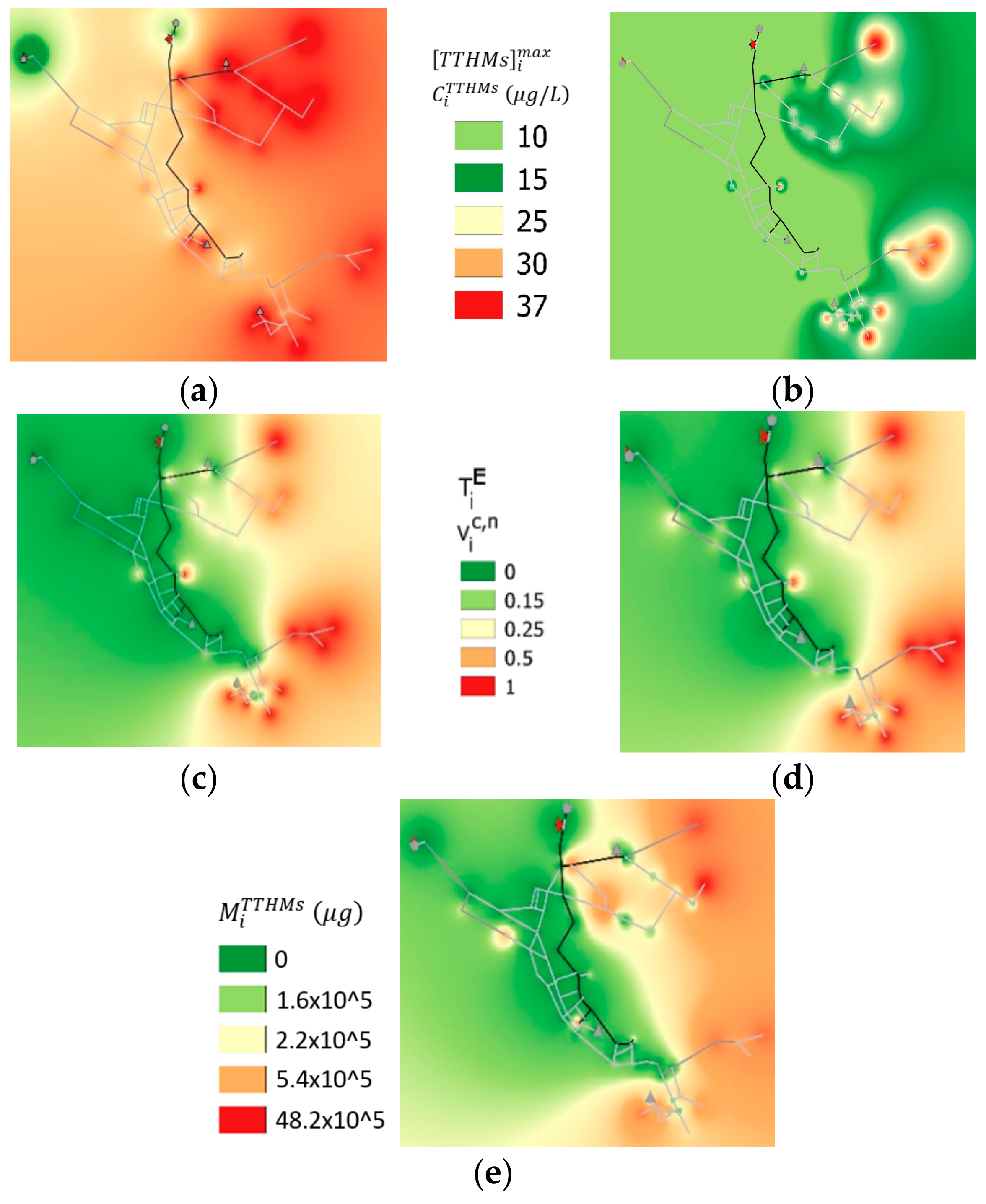
Figure 2 presents the vulnerability contour plot maps obtained for the five considered indexes. The maps furnish complementary information about the different kind of exposure that they describe. Considering [TTHMs]_i^max and C_i^TTHMs (Figure 2a,b), the green regions represent the “safe” zones, where the [TTHMs]_lim is never exceeded. The vulnerable nodes identified with C_i^TTHMs, from yellow to red areas, are less than the ones identified considering [TTHMs]_i^max, because the latter parameter is more restrictive and considers the node as critical even if the imposed limit has been exceeded only at one time step. In particular, 59 nodes reach during the day a TTHMs concentration above the limit, while C_i^TTHMs values above the threshold are registered in only 18 nodes. In particular, the nodes 131, 166, and 243 have the maximum C_i^TTHMs, which is approximately equal to 37 μg/L. Moreover, the highest values of both [TTHMs]_i^max and C_i^TTHMs are registered in node 243.

As expected, the maps obtained with V_i^c,n and T_i^E (Figure 2c,d) are very similar, indicating that there are eight nodes (the red ones) in which the limit concentration is exceeded for all of the simulation period (V_i^c,n = T_i^E = 1). All of these nodes are characterized by high water age values. In this group, the node 243 is also included.

Finally, the computed M_i^TTHMS values range from 277 μg to about 485 × 10⁴ μg, as reported in Figure 2e. The vulnerability map is slightly different from the other ones, and node 15, which is not included in the ones selected through V_i^c,n and T_i^E, is individuated as the most vulnerable one. In fact, in this node, the water age is lower, but the base demand, representing the daily mean values of the outputs in the node, is higher, indicating a large number of users.

3.2. PW06 Network

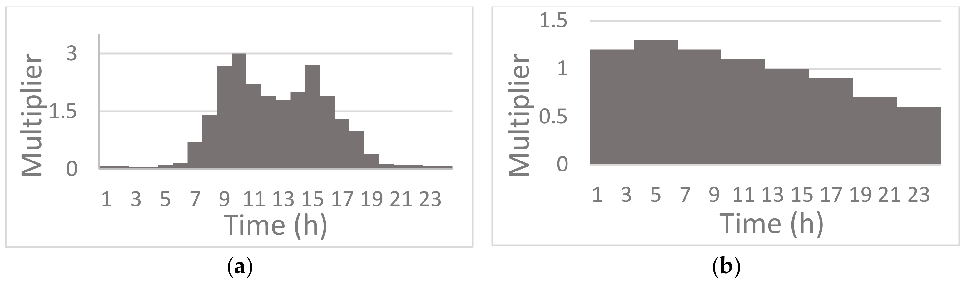
The PW06 network (Figure 1b) has 47 pipes and 33 demand nodes with elevations that vary between 10–30 m, and it is supplied from a single source (reservoir), where sodium hypochlorite is supposed to be injected. The base demands are half of the ones reported in the original paper, and the demand pattern of Figure 3a has been assigned in all of the nodes. The Hazen–Williams law is adopted as the resistance formula.

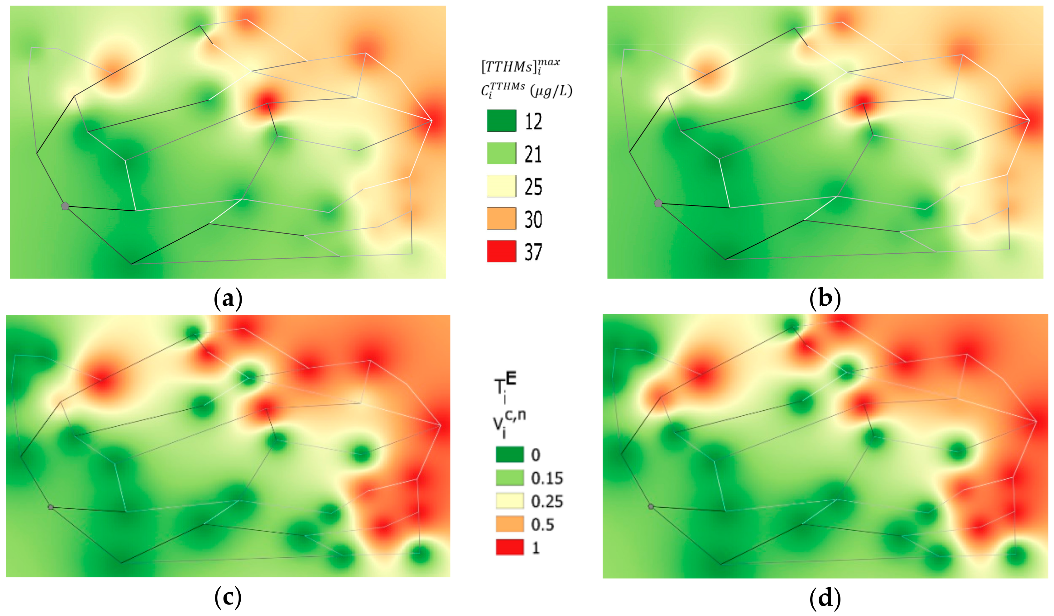
Unlike the Net-3 system, in this case study, the [TTHMs]_i^max and C_i^TTHMs values are very similar, as shown from the heat maps reported in Figure 4a,b. For both parameters, the limit is exceeded in the same 13 nodes, and they identify node 15 as the most vulnerable one.

As in the Net-3 case, the heat maps of T_i^E and V_i^c,n, as reported in Figure 4c,d, are similar, with 10 nodes in which the limit concentration is exceeded for the entire simulation period (V_i^c,n = T_i^E = 1). They are located in the opposite side with respect to the source, where the water ages have larger values. Also, the mass parameters individuate the same vulnerable area (Figure 4e), and the maximum M_i^TTHMS value (M_i^TTHMS = 14,053 × 10³ µg) is registered in node 7, which is included in the critical nodes selected through V_i^c,n and T_i^E.

3.3. Anytown Network

The Anytown water distribution system (Figure 1c) has 16 junctions, two tanks, 34 pipes, three pumps, and one reservoir, where sodium hypochlorite is supposed to be injected. The network has been partially modified for the purposes of the paper. In particular, in the nodes 20, 50, 60, 80, and 130, the base demands have been reduced by one third with respect to the original values, and the pattern in Figure 3b has been assigned, while for the rest of the nodes, the base demands have been reduced by one fifth with respect to the original values, and the demand pattern of Figure 3a has been used. The Hazen–Williams law is adopted as the resistance formula for the simulation.

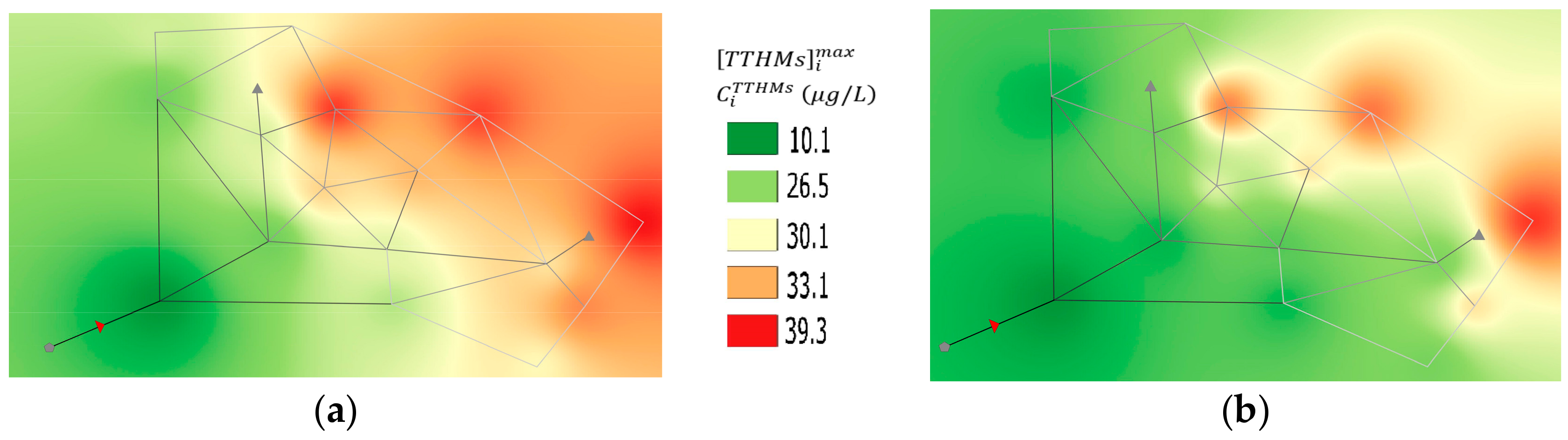
Figure 5 depicts the heat maps obtained with the five considered parameters. In this case study, unlike PW06, [TTHMs]_i^max and C_i^TTHMs identify the same critical nodes, but the values that they assume are very different, as indicated from heat maps in Figure 5a,b. In 13 nodes, the TTHMs concentration exceeds the limit, while the C_i^TTHMs reaches the threshold in only six nodes. For both parameters, the most critical node is the number 170, which is located far from the source. Similarly to the Net-3 network, the comparison between Figure 5a and Figure 5b indicates that the maximum concentration is a more restrictive parameter.

The parameters T_i^E and V_i^c,n individuate the same nodes as critical, but their values are different, as indicated from the heat maps of Figure 5c,d. In particular, the values of the dimensionless exposure time are lower than the ones of the normalized contaminated volume. The limit concentration is exceeded for the entire simulation period (V_i^c,n = T_i^E = 1) in only nodes 140 and 170.

The heat map corresponding to the parameter M_i^TTHMS reported in Figure 5e is slightly different from the other ones, and the maximum value (M_i^TTHMS = 41,756 × 10³ µg) is observed at node 80, which is not included in the ones individuated from the other parameters.

3.4. Aurunci Valcanneto Water Supply System (AVWSS)

The considered main trunk of the AVWSS is located in the Lazio region, and it serves about 110,000 inhabitants distributed among 25 towns. As shown in Figure 1d, the system is supplied by three sources (inlet nodes 1, 12, and 13), and water is delivered in nine outlet nodes, which represent the insertion into nine different WDSs.

In November 2008, a campaign of water quality measurements was realized, and the measured values of chlorine and TTHMs concentrations ([Cl₂]_m and [TTHMs]_m) are reported in

Table 1. Water quality measurements of November 2008 and the results of the vulnerability analysis.

Node Number	Age (h)	Q (L/s)	[Cl2]m (mg/L)	[TTHMs]m (µg/L)	[TTHMs]imax (µg/L)	TiE	MiTTHMs (103 µg)
2	0.17	2	0.27	1.97	0.04	0	0
3	1.89	8	0.27	1.49	0.46	0	0
4	3.92	2	-	-	0.94	0	0
5	6.85	2	0.26	1.32	1.65	1	26.28
6	5.98	8	-	-	1.45	0	0
7	6.37	2.5	-	2.00	1.54	1	9.33
8	8.57	3	-	2.45	2.03	1	138.36
9	18.06	47	0.24	3.02	3.91	1	9823.64
10	8.2	112	0.25	-	3.20	1	16,460.44

. A better description of the AVWSS can be found in Di Cristo et al. [36], where the system has been used as a case study to compare and validate some empirical and kinetics models for the prediction of the TTHMs concentration.

The demands in the delivering nodes are reported in Table 1, and no pattern is assigned, since the AVWSS is a main trunk. The simulation is performed in steady condition, and the obtained water age in the nodes are reported in Table 1. The limit considered on TTHMs concentration is 1.5 µg/L, which is fixed considering the extension of the WDSs connected to the outlet nodes. In other words, this threshold corresponds to about the 25 μg/L at the more distant outputs nodes of the connected WDSs. The initial chlorine concentration is 0.30 mg/L, while the TTHMs one is null. The reaction rate coefficients to model chlorine decay, k_b (Equation (7)), and TTHMs formation, D (Equation (8)), are fixed through a specific calibration equal to 0.02 1/h and 43 µg/mL, respectively.

Without a pattern in the nodes, the parameter C_i^TTHMs does not make sense, and T_i^E and V_i^c,n are coincident. As shown in Table 1, the results of the vulnerability analysis identify different critical nodes according to the different indexes. In particular, [TTHMs]_i^max selects node 9 as the most vulnerable one (with a maximum value of 3.91 µg/L), which corresponds to the node with the maximum water age. T_i^E assume the value 0 in four nodes where the [TTHMs]_lim has never been exceeded, and 1 in the nodes 5, 7, 8, 9, 10, corresponding to ages higher than 6 h. In terms of mass, the maximum value is delivered in node 10, with the maximum base demand (M_i^TTHMs = 16,460.44 × 10³ µg), which is included in the group identified by T_i^E.

3.5. Cimitile Network

Figure 1e reports the scheme of the water distribution network of Cimitile, a small town located in the Campania region in Southern Italy. The system, which serves about 3700 residents located in 2.74 km², consists of 433 pipes, with a total length of approximately 20 km, five regulation valves, and 404 junction nodes. Pipe diameters range from 20 mm to 260 mm. Predominant pipe materials are cast iron and steel, while there is only a small percentage of high-density polyethylene (HDPE) pipes. The water comes from a regional main trunk (not reported in the scheme) and it goes into the system through three inlet nodes (Gescal, Galluccio, and Pisacane).

Base demands values, as shown in the scheme of Figure 6 have been obtained working out utility consumption billing data, and the daily total flow rate supplied to the users is about 34.25 m³/s. The same water demand pattern, as characterized by two main peaks (Figure 3a), has been assigned to all of the nodes. The Darcy–Weisbach head loss formula is used for the simulation, and the hydraulic parameters have been previously calibrated using tank levels and pressure measurements. The chlorination of the water occurs in the three inlet nodes.

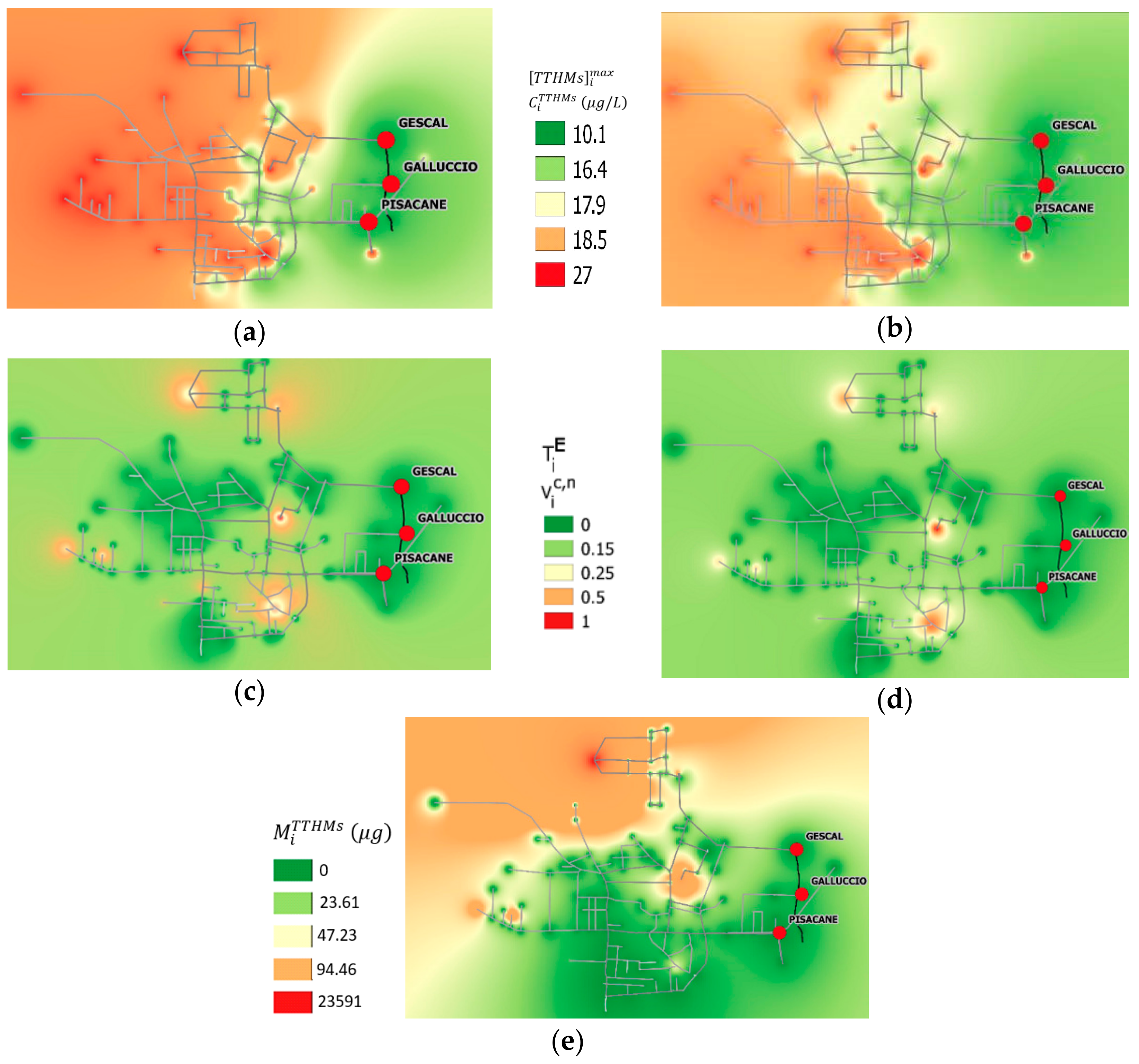
The vulnerability contour plot maps, as reported in Figure 7, indicate that also in this case, the vulnerable indexes tend to identify different risk areas considering different kinds of exposure. For a better understanding, Figure 6 reports the scheme of the network with the more vulnerable nodes selected using the different indexes. Moreover, Figure 8 illustrates the temporal variability of the TTHMs concentration in nodes 211, 290, and 328.

In terms of [TTHMs]_i^max and C_i^TTHMs (Figure 7a,b), the most critical nodes are located in the west part of the network. The number of nodes characterized by the excess of the attention limit in terms of maximum actual TTHMs concentration are more copious, because, as already mentioned, this parameter leads to also classifying as vulnerable those nodes where the [TTHMs]_lim is exceeded only once during the simulation time. Both parameters individuate the node 211 as the most critical one (Figure 6), in which the maximum C_i^TTHMs is about 27 μg/L. Furthermore, the same node 211 is located in the area of the network that is characterized by the highest water ages.

The heat maps show that the exposure time and the normalized contaminated volume (Figure 7c,d) enable identifying the same critical areas in the system. In particular, the zones with high T_i^E and V_i^c,n values are located in the north, central, and south parts of the network, and the lower and higher residence times nodes are equally involved. In five nodes 7, 211, 212, 242, and 328 (Figure 6), the concentration exceeds the limit for the entire simulation period (V_i^c,n = T_i^E = 1).

The M_i^TTHMs values range from 600 × 10³ μg at node 214 to about 23 × 10¹² μg at node 290 (Figure 7e). The high values of this parameter coincide with nodes characterized by large base demands, namely with a high number of users served. Using this index, the most vulnerable is node number 290, which is located in northwest region of the network, and is not included in the group individuated by the other parameters (Figure 6).

Figure 8 reports the TTHMs concentration time variability during the simulating day for the nodes 211, 290, and 328, identified as the most vulnerable during the analysis.

In node 290, which is identified as the most critical one according to M_i^TTHMs, the TTHMs concentration exceeds the attention limit for about 8 h at the beginning of the simulation and in the last few minutes. In the other considered nodes, 211 and 328, which are vulnerable according to all of the parameters except M_i^TTHMs, the TTHMs concentration are always above the threshold fixed at 25 μg/L, reaching a maximum value of around 27 μg/L in node 211. These results indicate that in the area of node 290, many users were exposed to a high concentration for a short period, while in the areas of nodes 211 and 328, fewer consumers were always exposed to TTHMs concentrations above the fixed threshold. This kind of analysis is very useful for optimizing the network management for better water quality.

4. Conclusions

Water distribution vulnerability to elevated TTHMs concentrations is explored through the use of five different indexes that enable evaluating the population’s exposure. The methodology is applied to five case studies: three literature schemes—namely Net-3, PW06, and Anytown—and two real systems, namely AVWSS and Cimitile, which are both located in Italy.

The main outcome of the obtained results is that the introduced indexes identify different critical areas with respect to elevated TTHMs concentrations, depending on the kind of exposure to which they refer. They enable identifying the higher risk nodes with respect to the different kinds of exposure: high concentration exposure for a short period, or chronic exposure to low TTHMs concentrations. The comparison between the maps obtained from the different indexes suggests that their performances strongly depend on the behavior of the system.

The presented research is significant because vulnerability analyses are important for water companies and administrators to design public health and strategies to reduce risks. The proposed methodology provides valuable information for assisting water utilities in the WDSs management considering water quality. In particular, the results of the presented study and the information embedded are also effective in the implementation of methodologies for the formulation of optimization problems such as chlorine dosage or chlorine booster allocation in the system or for planning network modifications. The vulnerability indexes can also be adopted for performing the district sectorization and skeletonization of a network accounting for water quality. Moreover, even if it is presented considering the TTHMs, the proposed methodology can be used for evaluating the exposure to others DPBs, adopting the adequate modelling for predicting the concentration and selecting the relative threshold limit.