Hydrological Analysis of a Dyke Pumping Station for the Purpose of Improving Its Functioning Conditions


Abstract
:1. Introduction
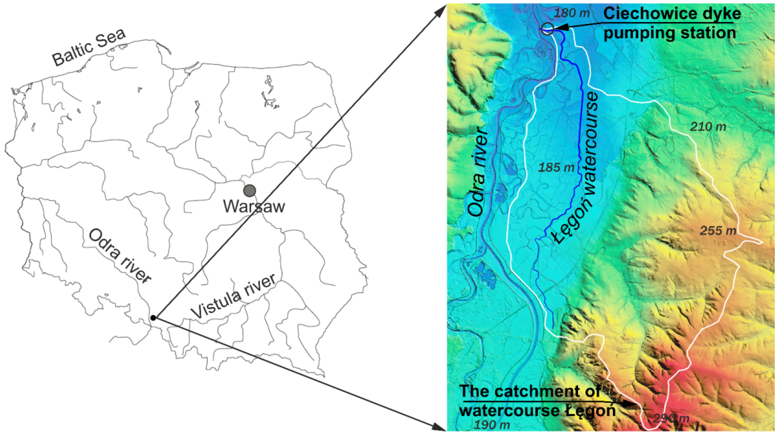
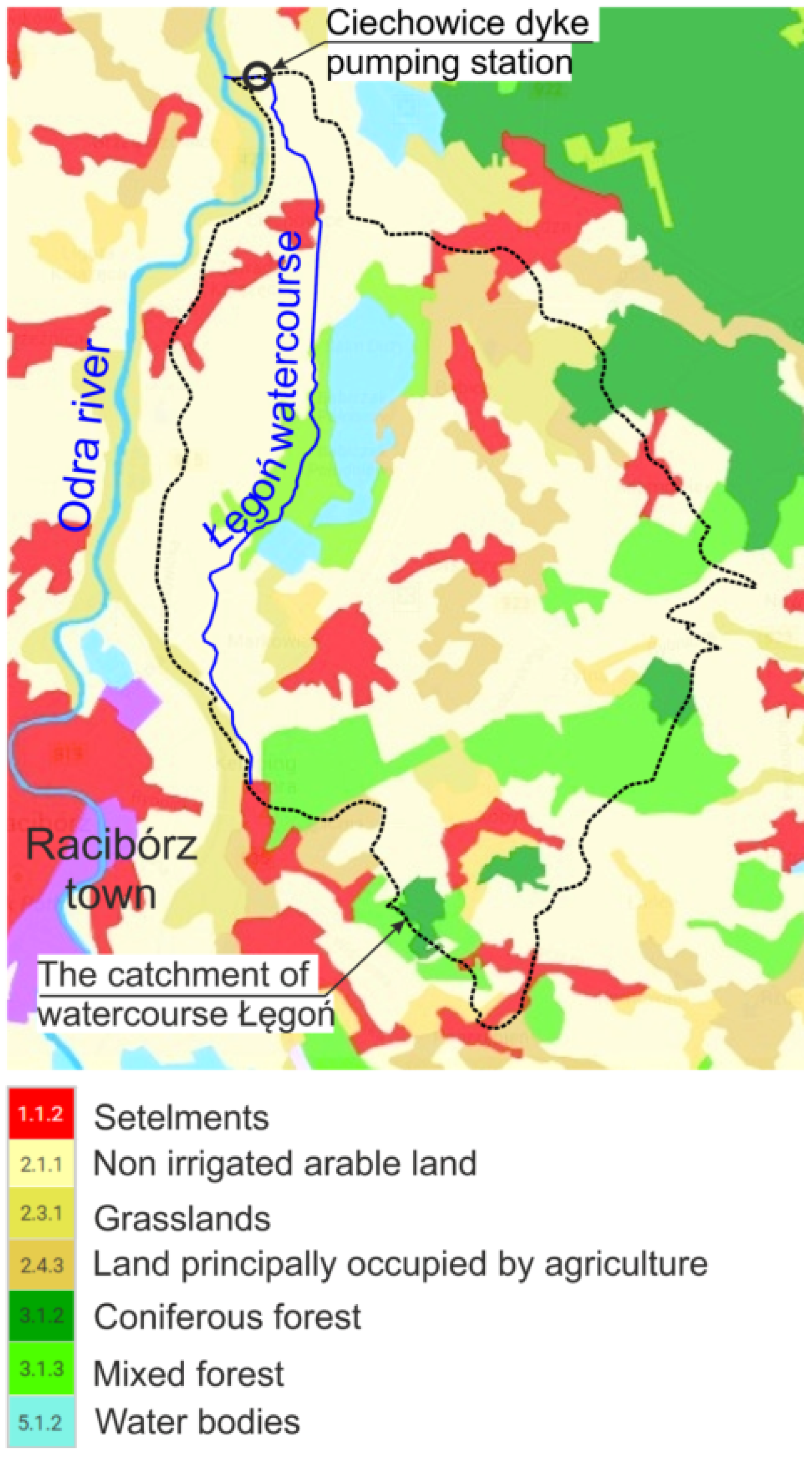
2. Study Area
3. Methodologies of Flows Estimation
3.1. Design Flows—The Spatial Regression Equation
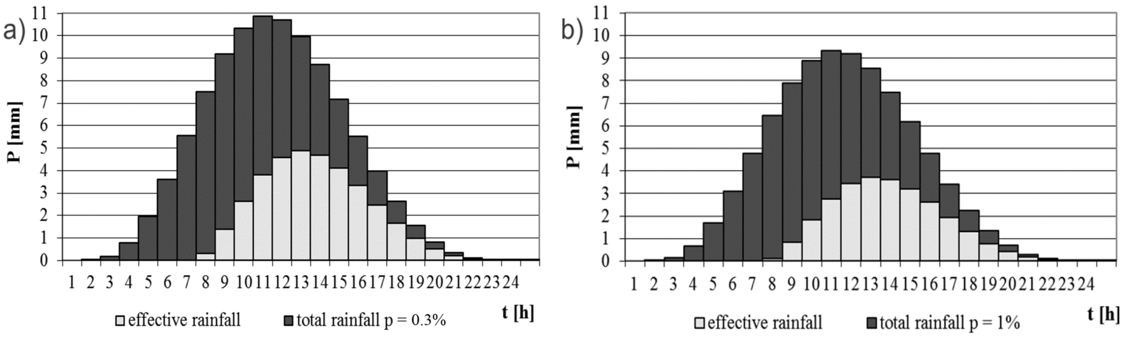
3.2. The NRCS-CN Method
| Fraction of precipitation time [h] | (0–0.3)T | (0.3–0.5)T | (0.5–1.0)T |
| Percentage of total precipitation | 20 | 50 | 30 |
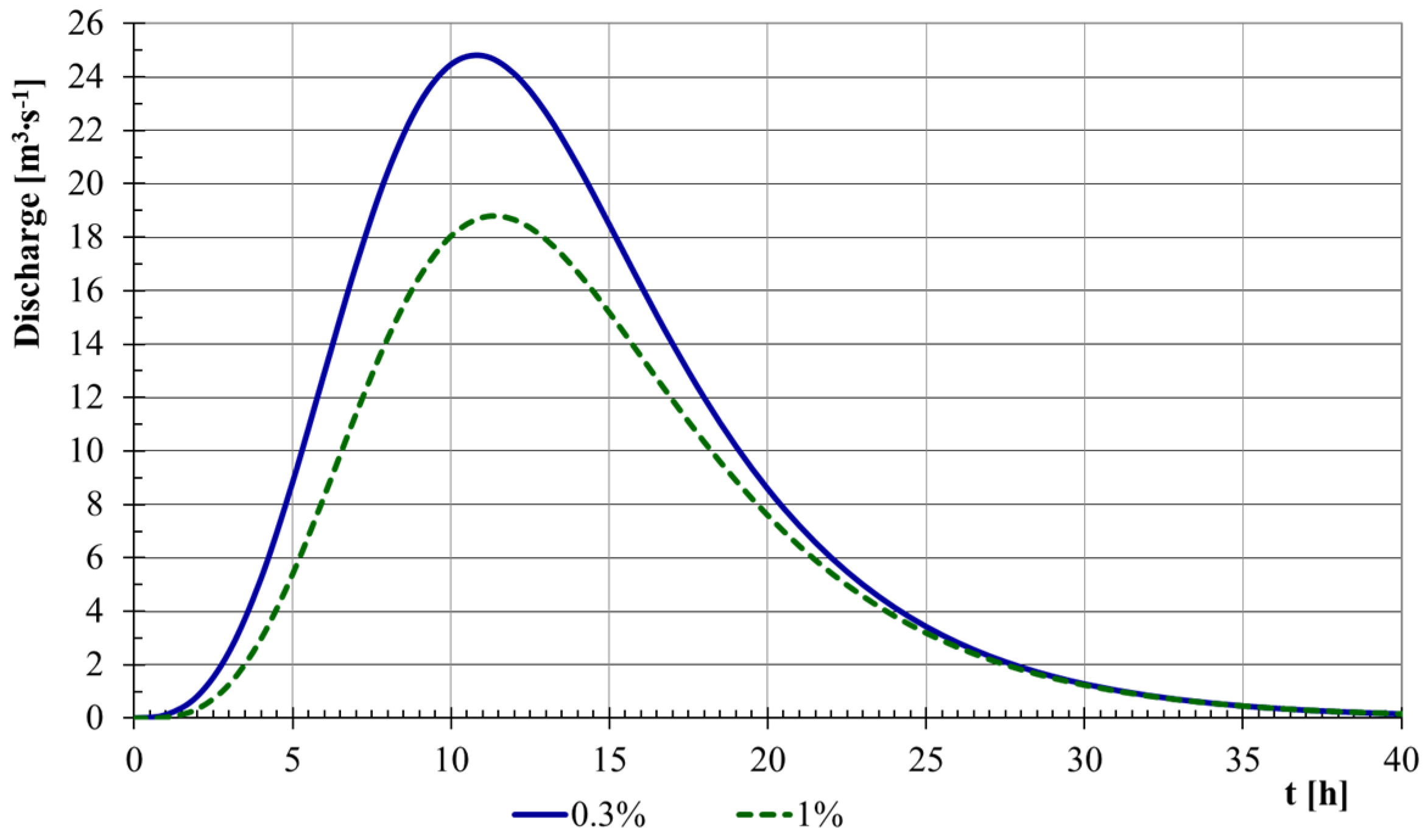
3.3. Determination of Wave Hydrographs
3.4. Flood Waves Routing
3.5. Methodology Summary
- Selecting the methodology for estimating calculated flows with a specified probability of exceedance, which depends on whether the catchment is being controlled or not.
- Conducting hydrological calculations for designing flows estimation.
- Generating hydrographs to calculate flows.
- Evaluating terrain conditions in the localization of a dyke pumping station, which enables a retarding reservoir with a determined capacity and parameters to be constructed.
- Selecting the capacity of pumps in the dyke pumping station.
- Selecting computational scenarios that consider the variable capacity of pumps and the variable volume of a retarding reservoir.
- Estimating the functioning conditions of a dyke pumping station and a retarding reservoir during the occurrence of a flood wave.
- Estimating the costs of construction, exploitation, and maintenance for a dyke pumping station and a retarding reservoir with regards to different computational scenarios.
4. Pump Station Capacity Assumptions
- in each of the calculation cases, the retarding reservoir bottom is situated at 174.60 m a.s.l.,
- the retarding reservoir side slope is 1:2,
- the normal drainage level is 176.30 m a.s.l.,
- the maximum allowable water level in the upper dyke areas is 178.00 m a.s.l.,
- the dyke culvert flaps are closed (there is a flood on the main river),
- the initial water level in the retarding reservoir is situated at 176.00 m a.s.l.,
- the pump switching on/off levels: I-176.30/175.80; II-176.70/176.20; III-177.10/177.60; IV-177.50/177.00.
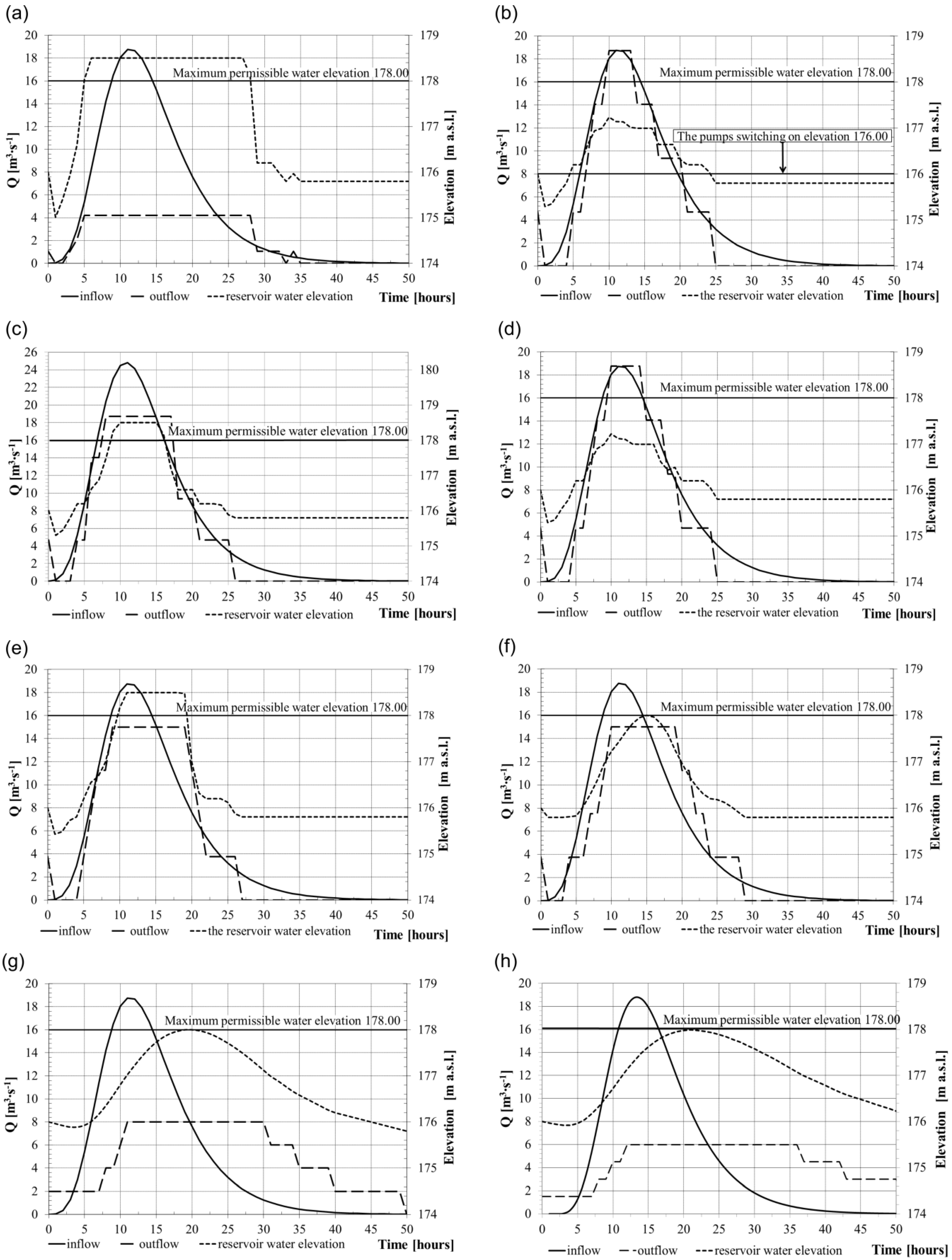
- Case 1: current (existing) state, retarding reservoir bottom dimensions of 15 × 100 m, pumps’ output of 4 × 0.9 = 3.60 m3 s−1, design flood wave routing;
- Case 2: current state, retarding reservoir bottom dimensions of 15 × 100 m, pumps’ output after alteration of 4 × 1.05 = 4.20 m3 s−1, design flood wave routing;
- Case 3: a total pumping station capacity of 18.75 m3 s−1, four pumps as is the case for the current state, four additional pumps with a capacity of 15.15 m3 s−1, retarding reservoir bottom dimensions of 45 × 240 m, design flood wave routing;
- Case 4: a total pumping station capacity of 18.75 m3 s−1, four pumps as is the case for the current state, four additional pumps with a total capacity of 15.15 m3 s−1, retarding reservoir bottom dimensions of 45 × 240 m, control flood wave routing;
- Case 5: a total pumping station capacity of 18.75 m3 s−1, four pumps after alteration 4 × 1.05 = 4.20 m3 s−1, four additional pumps with a capacity of 14.55 m3 s−1, retarding reservoir bottom dimensions of 45 × 240 m, design flood wave routing;
- Case 6: a total pumping station capacity of 15.0 m3 s−1, four pumps, retarding reservoir bottom dimensions of 45 × 240 m, design flood wave routing;
- Case 7: a total pumping station capacity of 15.0 m3 s−1, four pumps, retarding reservoir bottom dimensions of 55 × 910 m, design flood wave routing;
- Case 8: a total pumping station capacity of 8.0 m3 s−1, four pumps, retarding reservoir bottom dimensions of 100 × 1700 m, design flood wave routing;
- Case 9: a total pumping station capacity of 6.0 m3 s−1, four pumps, retarding reservoir bottom dimensions of 100 × 2150 m, design flood wave routing.
5. Calculation Results and Discussion
6. Conclusions
- The designed flood wave of p = 1% cannot be safely passed through the pumping station for the existing specifications—the total pumping station capacity of 3.60 m3 s−1 and the retarding reservoir capacity of 7412 m3.
- On the basis of computer simulations, it should be indicated that the solution that involves reducing the required pumping station capacity leads to an increase in the required retarding reservoir capacity. The approach to ensure safe operation of the pumping station should not only take into consideration the capacity of the pumping station and volume of the retarding reservoir, but also the retention capacity of the riverbed. This will reduce the cost of rebuilding an existing facility.
- On the basis of the performed analysis, it was decided that Case 5 is the most beneficial for reconstructing the dyke pumping station, and in this case, the designed flood wave of p = 1% can be safely passed through the Ciechowice pumping station at the total pumping station capacity of 18.75 m3 s−1 and the retarding reservoir capacity of 31,590 m3.
Author Contributions
Conflicts of Interest
References
- Szolgay, J.; Gaál, L.; Bacigál, T.; Kohnová, S.; Hlavčová, K.; Výleta, R.; Parajka, J.; Blöschl, G. A regional comparative analysis of empirical and theoretical flood peak-volume relationships. J. Hydrol. Hydromech. 2016, 64, 367–381. [Google Scholar] [CrossRef] [Green Version]
- Grimaldi, S.; Petroselli, A. Do we still need the Rational Formula? An alternative empirical procedure for peak discharge estimation in small and ungauged basins. Hydrol. Sci. J. J. Sci. Hydrol. 2015, 60, 67–77. [Google Scholar] [CrossRef]
- Wan, Y.; Konyha, K. A simple hydrologic model for rapid prediction of runoff from ungauged coastal catchments. J. Hydrol. 2015, 528, 571–583. [Google Scholar] [CrossRef]
- Castiglioni, S.; Lombardi, L.; Toth, E.; Castellarin, A.; Montanari, A. Calibration of rainfall-runoff models in ungauged basins: A regional maximum likelihood approach. Adv. Water Resour. 2010, 33, 1235–1242. [Google Scholar] [CrossRef]
- Hughes, D.A.; Slaughter, A. Daily disaggregation of simulated monthly flows using different rainfall datasets in Southern Africa. J. Hydrol. Reg. Stud. 2015, 4, 153–171. [Google Scholar] [CrossRef]
- Hughes, D.A. Simulating temporal variability in catchment response using a monthly rainfall–runoff model. Hydrol. Sci. J. J. Sci. Hydrol. 2015, 60, 1286–1298. [Google Scholar] [CrossRef]
- Hughes, D.A.; Slaughter, A. Disaggregating the components of a monthly water resources system model to daily values for use with a water quality model. Environ. Model Softw. 2016, 80, 122–131. [Google Scholar] [CrossRef]
- Jiang, Y.; Liu, C.; Li, X.; Liu, L.; Wang, H. Rainfall-runoff modelling, parameter estimation and sensitivity analysis in a semiarid catchment. Environ. Model Softw. 2015, 67, 72–88. [Google Scholar] [CrossRef]
- Soulis, K.X.; Valiantzas, J.D.; Dercas, N.; Londra, P.A. Investigation of the direct runoff generation mechanism for the analysis of the SCS-CN method applicability to a partial area experimental watershed. Hydrol. Earth Syst. Sci. 2009, 13, 605–615. [Google Scholar] [CrossRef] [Green Version]
- Ajmal, M.; Waseem, M.; Ahn, J.-H.; Kim, T.-W. Improved Runoff Estimation Using Event-Based Rainfall-Runoff Models. Water Resour. Manag. 2015, 29, 1995–2010. [Google Scholar] [CrossRef]
- Soulis, K.X.; Valiantzas, J.D. SCS-CN parameter determination using rainfall-runoff data in heterogeneous watersheds—The Two-CN system approach. Hydrol. Earth Syst. Sci. 2012, 16, 1001–1015. [Google Scholar] [CrossRef] [Green Version]
- Jiao, P.; Xu, D.; Wang, S.; Yu, S.; Han, S. Improved SCS-CN Method Based on Storage and Depletion of Antecedent Daily Precipitation. Water Resour. Manag. 2015, 29, 4753–4765. [Google Scholar] [CrossRef]
- Leopardi, M.; Scorzini, A.R. Effects of wildfires on peak discharges in Watersheds. iForest-Biogeosci. For. 2015, 8, 302–307. [Google Scholar] [CrossRef]
- Taher, T.M. Integration of GIS Database and SCS-CN Method to Estimate Runoff Volume of Wadis of Intermittent Flow. Arab. J. Sci. Eng. 2015, 40, 685–692. [Google Scholar] [CrossRef]
- Verma, S.; Verma, R.K.; Mishra, S.K.; Singh, A.; Jayaraj, G.K. A revisit of NRCS-CN inspired models coupled with RS and GIS for runoff estimation. Hydrol. Sci. J. 2017, 62, 1891–1930. [Google Scholar] [CrossRef]
- Kousari, M.R.; Malekinezhad, H.; Ahani, H.; Zarch, M.A.A. Sensitivity analysis and impact quantification of the main factors affecting peak discharge in the SCS curve number method: An analysis of Iranian watersheds. Quat. Int. 2010, 226, 66–74. [Google Scholar] [CrossRef]
- Fan, F.; Deng, Y.; Hu, X.; Weng, Q. Estimating Composite Curve Number Using an Improved SCS-CN Method with Remotely Sensed Variables in Guangzhou, China. Remote Sens. 2013, 5, 1425–1438. [Google Scholar] [CrossRef] [Green Version]
- Tramblay, Y.; Bouvier, C.; Martin, C.; Didon-Lescot, J.-F.; Todorovik, D.; Domergue, J.-M. Assessment of initial soil moisture conditions for event-based rainfall–runoff modeling. J. Hydrol. 2010, 387, 176–187. [Google Scholar] [CrossRef]
- Nash, J.E. A unit hydrograph study with particular reference to British catchments. Proc. Inst. Civ. Eng. 1960, 17, 249–282. [Google Scholar] [CrossRef]
- Nash, J.E.; Sutcliffe, J.V. River Flow Forecasting through Conceptual Models. Part I—A Discussion of Principles. J. Hydrol. 1970, 10, 282–290. [Google Scholar] [CrossRef]
- Jaiswal, R.K.; Thomas, T.; Galkate, R.V.; Ghosh, N.C.; Lohani, A.K.; Kumar, R. Development of Geomorphology Based Regional Nash Model for Data Scares Central India Region. Water Resour. Manag. 2014, 28, 351–371. [Google Scholar] [CrossRef]
- Nourani, V. A Comparative Study on Calibration Methods of Nash’s Rainfall-Runoff Model to Ammameh Watershed, IRAN. J. Urban Environ. Eng. 2008, 2, 14–20. [Google Scholar] [CrossRef] [Green Version]
- Szilagyi, J. State-Space Discretization of the Kalinin-Milyukov-Nash-Cascade in a Sample-Data System Framework for Streamflow Forecasting. J. Hydrol. Eng. 2003, 8, 339–347. [Google Scholar] [CrossRef]
- Stachy, J.; Fal, B. The rules of calculation of maximal probable flows. The spatial regression equation. Gospodarka Wodna 1987, 1, 8–13. (In Polish) [Google Scholar]
- DVWK. Ermittlung der Verdunstung von Land- und Wasserflachen; Merkblatter zur Wasserwirtschaft: Bonn, Germany, 1996; p. 238. [Google Scholar]
- Hawkins, R.H.; Jiang, R.; Woodward, D.E.; Hjelmfelt, A.T.; Van Mullem, J.A.; Quan, Q.D. Runoff Curve Number Method: Examination of the Initial Abstraction Ratio, In Proceedings of the Second Federal Interagency Hydrologic Modeling Conference, Las Vegas, NV, USA, 28 July–1 August 2002; ASCE: Lakewood, CO, USA, 2002.
- Nigam, G.K.; Sahu, R.K.; Sinha, M.K.; Deng, X.; Singh, R.B.; Kumar, P. Field assessment of surface runoff, sediment yield and soil erosion in the opencast mines in Chirimiri area, Chhattisgarh, India. Phys. Chem. Earth 2017, 101, 137–148. [Google Scholar] [CrossRef]
- Chung, W.H.; Wang, I.T.; Wang, R.Y. Theory-Based SCS-CN Method and Its Applications. J. Hydrol. Eng. 2010, 15, 1045–1058. [Google Scholar] [CrossRef]
- Ponce, V.M. Engineering Hydrology: Principles and Practices; Preutice Hall: Upper Saddle River, NJ, USA, 1989. [Google Scholar]
- Zakizadeh, F.; Malekinezhad, H. Comparison of Methods for Estimation of Flood Hydrograph Characteristics. Russ. Meteorol. Hydrol. 2015, 40, 12. [Google Scholar] [CrossRef]
- Jain, S.C. Open-Channel Flow; John Wiley & Sons Inc.: New York, NY, USA, 2001. [Google Scholar]
- Bačová Mitková, V.; Pekárová, P.; Miklánek, P.; Pekár, J. Hydrological simulation of flood transformations in the upper Danube River: Case study of large flood events. J. Hydrol. Hydromech. 2016, 64, 337–348. [Google Scholar] [CrossRef] [Green Version]


| Soil | % Area | Hydrologic Soil Group |
|---|---|---|
| Sediments | 12.8 | A |
| Peat | 13.58 | C |
| Sand | 31.39 | B |
| Sandy loam | 28.9 | C |
| Loess and silt | 8.23 | B |
| Water | 5.1 | - |
| Type | A (km2) | % Area |
|---|---|---|
| Agricultural areas | 29.37 | 59.45 |
| Grasslands | 1.71 | 3.47 |
| Mixed forest | 8.22 | 16.65 |
| Coniferous forest | 1.44 | 2.92 |
| Settlement | 6.15 | 12.44 |
| Water | 2.50 | 5.07 |
| Total catchment area | 49.4 | 100 |
| Case | Bottom Dimensions [m × m] | Reservoir Capacity [m3] | Reservoir Depth [m] | Max. Water Elevation in the Reservoir [m a.s.l.] | Capacity of the Pumping Station [m3 s−1] |
|---|---|---|---|---|---|
| 1 | 15 × 100 | 7412 | - | above 178.00 | 4 × 0.9 = 3.60 |
| 2 | 15 × 100 | 7412 | - | above 178.00 | 4 × 1.05 = 4.20 |
| 3 | 45 × 240 | 31,724 | 2.63 | 177.23 | 4 × 0.9 + 15.16 = 18.76 |
| 4 | 45 × 240 | - | - | above 178.00 | 4 × 0.9 + 15.16 = 18.76 |
| 5 | 45 × 240 | 31,591 | 2.62 | 177.22 | 4 × 1.05 + 14.46 = 18.76 |
| 6 | 45 × 240 | - | - | above 178.00 | 4 × 3.75 = 15.00 |
| 7 | 55 × 910 | 191,209 | 3.40 | 178.00 | 4 × 3.75 = 15.00 |
| 8 | 100 × 1700 | 617,304 | 3.40 | 178.00 | 4 × 2.0 = 8.00 |
| 9 | 100 × 2150 | 778,266 | 3.39 | 177.99 | 4 × 1.5 = 6.00 |
© 2018 by the authors. Licensee MDPI, Basel, Switzerland. This article is an open access article distributed under the terms and conditions of the Creative Commons Attribution (CC BY) license (http://creativecommons.org/licenses/by/4.0/).
Share and Cite
Machajski, J.; Kostecki, S. Hydrological Analysis of a Dyke Pumping Station for the Purpose of Improving Its Functioning Conditions. Water 2018, 10, 737. https://doi.org/10.3390/w10060737
Machajski J, Kostecki S. Hydrological Analysis of a Dyke Pumping Station for the Purpose of Improving Its Functioning Conditions. Water. 2018; 10(6):737. https://doi.org/10.3390/w10060737
Chicago/Turabian StyleMachajski, Jerzy, and Stanisław Kostecki. 2018. "Hydrological Analysis of a Dyke Pumping Station for the Purpose of Improving Its Functioning Conditions" Water 10, no. 6: 737. https://doi.org/10.3390/w10060737
APA StyleMachajski, J., & Kostecki, S. (2018). Hydrological Analysis of a Dyke Pumping Station for the Purpose of Improving Its Functioning Conditions. Water, 10(6), 737. https://doi.org/10.3390/w10060737