Time-Lapse Photography of the Edge-of-Water Line Displacements of a Sandbar as a Proxy of Riverine Morphodynamics

Abstract

A simple methodology to track the displacements of a sandbar from a fixed video camera, extracting its morphological features and deriving the associated fluvial morphology is presented, using a small reach of the Po River in Italy as a case study. A camera fixed on a bridge pier acquired images every twelve hours while hourly water levels are derived from a radar hydrometer located upstream of the study area. The quantification of the fluvial bathymetry is achieved by mapping multiple edge-of-water lines of a sandbar before and after high flow conditions in December 2017. Both from video information and 2-D numerical simulations, it is evident that flooding waves can easily remove sediments that accumulated on bars during low flow conditions in this area, redistributing them across the river channel. This video-based methodology—which confirms to be economically attractive if compared to more traditional monitoring systems—proves to be a valuable system to monitor long-term fluvial processes providing detailed indications on how to better plan river management activities.

1. Introduction

Since fluvial morphodynamics are a result of complex interactions between water flow, sediment transport, and riparian vegetation (e.g., [1,2,3,4]), the forecast of the channel cross-section evolution, the displacement of partially emerged bars or the quantification of the bank erosion could result difficult and typically requires for a detailed numerical modeling. The calibration of such models is needed for in-field data, which can be derived from topographic surveys. However, especially in the case of high flow conditions, this can become very challenging due to practical constraints. Therefore, improved monitoring techniques able to acquire information with a high resolution from remote distances are necessary, aiming to characterize the fluvial environment continuously and regardless the water stage and the atmospheric conditions. In the last decades, several techniques for monitoring coastal and riverine morphodynamics and edge-of-water line displacements have been employed by the scientific community, based on the use of kinematic DGPS (differential global positioning system), on the post-processing of historical maps [5], data remotely acquired by satellites [6,7,8,9], airplanes [10,11,12] or more recently, unmanned aerial vehicles [13], or on the analysis of video camera images [14,15].

Regarding this latter technique, since digital photogrammetry is becoming a major tool in monitoring landform evolution in riverine environments with nonintrusive techniques, due to its relatively reduced costs in comparison with other techniques [16,17] and the good resolution of the acquired images. Moreover, freeware software devoted to image analysis is spreading, encouraging non-experts to move toward photogrammetry and time-lapse photography to remotely monitor riverine morphodynamics at the three-dimensional scale [16,18]. Indeed, one of the main challenges is to transform two-dimensional distorted images captured by the camera into three-dimensional real-world coordinates to follow the edge-of-water line displacements. This methodology has been extensively used for the assessment of the coastal shore evolution [19,20] in the last 10–15 years, giving a tool for the monitoring and estimation of the erosive trend of beaches in the short- [21] and in the long-term [22]. The images acquired from local video camera stations have been used to calibrate and validate numerical codes with field observations, integrating early warning systems of coastal flooding [14,23] and for the management of hydraulic infrastructures located in alluvial rivers.

Compared to indicators derived from satellite imagery and proposed as a proxy for the impact of flooding events on the fluvial morphodynamics [24,25], datum-based edge-of-water line positioning has some specific advantages: (i) it is possible to visually interpret the evolution in terms of shifts and rotations; (ii) continuous images can be taken, even during flood peaks, thanks to the use of remote sensors; (iii) acquired images are more reliable in representing the landscape forms with respect to satellite images thanks to their higher resolution; (iv) it is a rather unsupervised and cheap approach, typically not interfering with the studied environment. Even if a limited number of specific topographic surveys with DGPS are required to calibrate the images for each case study, this method yields more efficient results than other techniques such as repeated topographic campaigns or analysis of satellite images. In fact, thanks to its affordable cost, it can be easily replicated to monitor large areas retrieving information on fluvial edge-of-water lines, having a good resolution and therefore sufficient to characterize the displacements of fluvial bedforms and overall river morphodynamics.

Using the small reach of the Po River (Italy) close to the city of Revere as a case study, the paper highlights the advantages in evaluating the edge-of-water line displacement captured remotely using a video camera as an indicator of the fluvial morphodynamics during a flooding event. After the description of the case study, the adopted methods are described, summarizing the main characteristics of the time-lapse photogrammetric approach and the numerical model applied to simulate the observed fluvial macro-dynamics. The results showed the qualitative agreement between the edge-of-water line evolution of the sandbar and the changes of a cross-section located downstream of the Revere Bridge due to a flooding event monitored with a fixed camera and numerically simulated with a 2-D freeware code. The accuracy of the photogrammetric approach is evaluated and discussed, and proposes possible improvements aimed to better track the edge-of-water line displacements and to reduce the errors associated with the homographic procedure. The conclusions summarized the research, pointing out the main advantages of using this method, as well as suggesting open questions for scholars and researchers that should be addressed for the future.

2. Materials and Methods

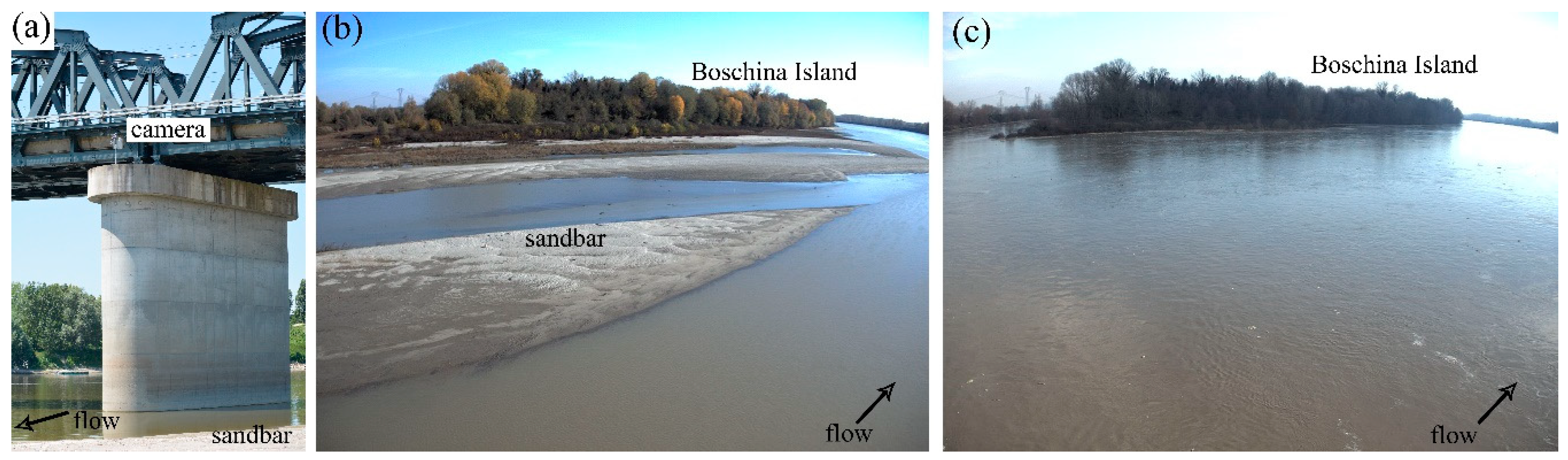
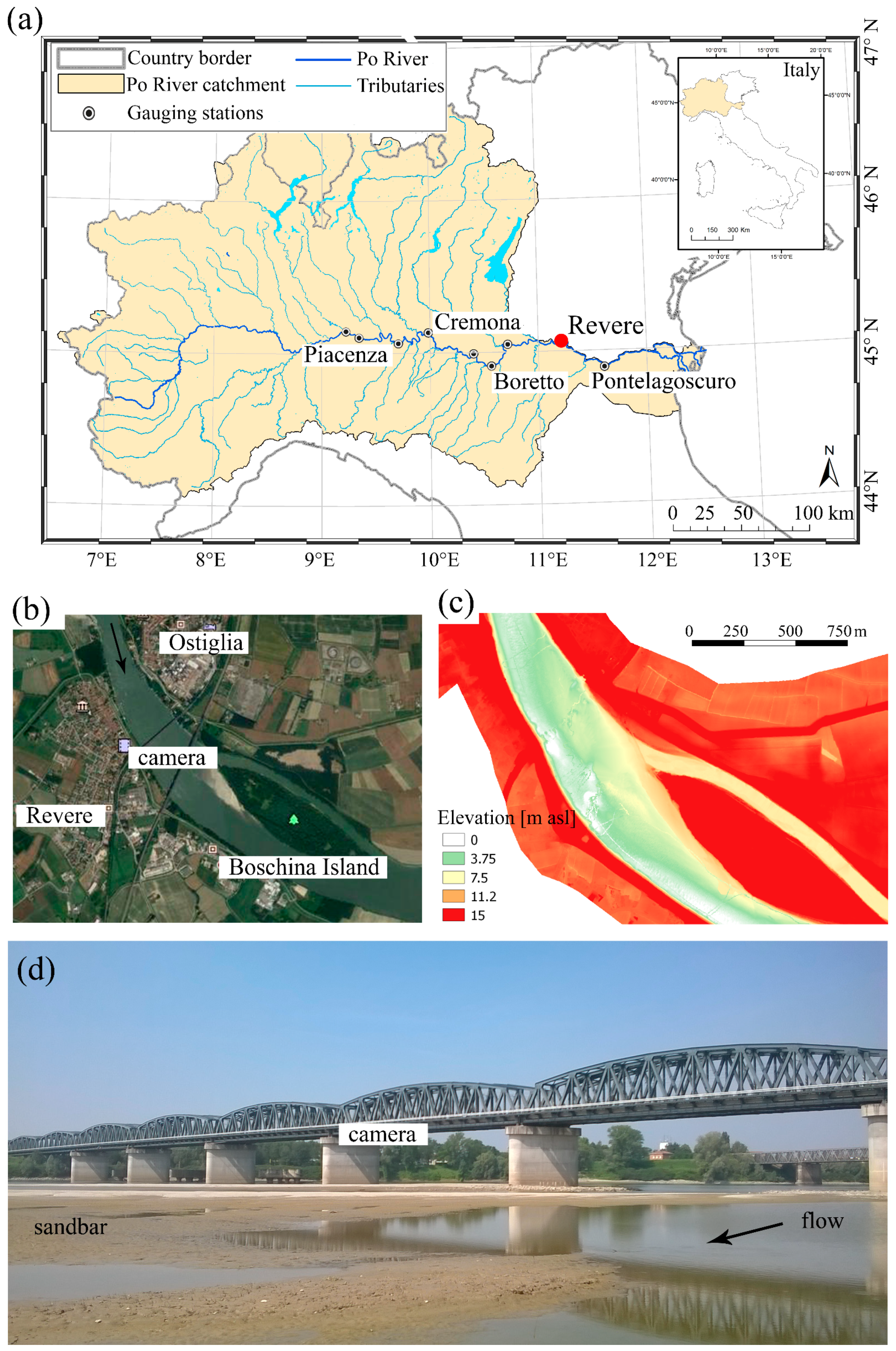
Remote imagery is frequently adopted in continuously monitoring the fluvial behaviour given the advantages of using non-invasive techniques and, combined with numerical modeling tools, offer the opportunity to forecast the future evolution of the riverine morphodynamics and eventually prevent hazards to hydraulic infrastructures.

In the present approach, the freeware suite iRIC 3.0, already calibrated and tested against field data representing a 10-km reach of the Po River [26] (Figure 1b) is applied to reproduce the behavior of a small region of the same reach forced by a flooding event. The edge-of-water line displacements of a sandbar observed with a fixed video camera installed on a bridge pier on the Po River (Italy) were coupled with hydrographic data measured at the same location to evaluate the capability of the proposed approach to reproduce the local fluvial morphology.

2.1. Case Study

The Po River, the longest watercourse in Italy, flows eastward across northern Italy for around 660 km (Figure 1a). Its drainage area measures about 74,500 km², of which 28,000 km² in mountain environments and the rest on the floodplain. The river catchment can be divided into three sectors based on the lithology and maximum elevation: an Alpine sector of crystalline and carbonate rocks (maximum relief ∼4500 m a.s.l.), an Apennine sector, mostly composed of sedimentary rocks with high clay content (maximum relief ∼2000 m a.s.l.) and a central alluvial area including the Po plain and the delta in the Adriatic Sea [27]. The middle and lower portions of this watercourse, flowing across strongly urbanized areas, are subjected to significant flood hazards and are consequently heavily embanked [24]. The annual hydrograph at the gauging station of Revere (circle, Figure 1a) shows two peaks in discharge, generally in autumn and spring, generated by rainfall and snowmelt, respectively, and the mean annual discharge is around 800–1000 m³/s; while the total annual sediment and freshwater discharges to the Northern Adriatic Sea were estimated at about 10–13 × 10⁹ kg and 40–50 km³, respectively [28,29,30]. The present river bathymetry results from the interaction between natural processes and anthropic activities acting along the reach for centuries. In fact, gravel and sand mining from the riverbed, combined with the creation of river embankments to prevent flooding and construction of hydropower reservoirs in the Alpine sector promoted a strong and long-lasting decrease in both the water flow and the sediment load [31,32]. Consequently, a significant degradation of the overall riverbed has been detected [26,33,34], particularly in the last decades [35].

The study area is located downstream of a railway bridge close to the city of Revere (Figure 1b), in a reach having a mean width of 400 m, a mean bed elevation of few meters above the sea level (Figure 1c), and a bed slope in the order of 10⁻⁵, which corresponds to the observed water slope between two hydrometers located upstream and downstream the area. The railway bridge where the camera is fixed is composed of seven piers, three of which are located within the river channel on the right side, where the waterway is located, while the other piers are characterized by local deposition during low flow conditions, being outside of the main current on the left side (Figure 1d).

2.2. Time-Lapse Photography

The edge-of-water line changes were monitored with a fixed camera Mobotix MX-M15D-SEC, remotely connected through a Sierra Wireless router, installed on June 2017 on a pier of the railway bridge between the cities of Revere and Ostiglia (coordinates 45°03′13.4″ N, 11°08′16.2″ E). Given that the pier is outside the river channel, it is reached by water only during high flow conditions (Figure 1d). The station consists of a single camera having two day/night sensors with a resolution of 12.5 megapixels (i.e., 960 × 1280 pixels) and a router remotely connected, allowing for a real-time monitoring and configuration. Images were acquired every 12 h, but only daily images are here compared to recognize the edge-of-water line displacements of the sandbar because of the better light conditions.

The image processing toolbox of MATLAB was used to correct the image distortion due to the camera lens [15,36], while the edge-of-water line features were extracted using a procedure developed for MATLAB. In addition, homographic equations were applied to transform image plane coordinates x,y to real plane coordinates x′,y′ [37,38] for each water elevation. That consists in a linear relationship between the two planes (Equation (1)):

$$\{\begin{array}{c}{x}^{\prime }=\frac{a_{11}x+a_{12}y+a_{13}}{a_{31}x+a_{32}y+a_{33}}\\ y^{\prime }=\frac{a_{21}x+a_{22}y+a_{23}}{a_{31}x+a_{32}y+a_{33}}\end{array}$$

(1)

The above relations give the coordinates (x′,y′) of each image pixel on the real plane, while the homographic coefficients “a_ij” can be computed if camera position and the coordinates of at least three points are known. In this application, a two-steps method was used, calibrating and validating the homographic coefficients a_ij (Figure 2b). First, during the training phase, by knowing the camera position and the actual coordinates (x′,y′) of five target points, a_ij are assessed by inverting Equation (1). Second, two additional targets points are used for testing the reliability of the calibrated method in predicting their real coordinates (x′,y′).

In Figure 2a, an image taken by the video station is presented. The edge-of-water lines extracted on the same day of the collection of the image (November 2nd, 2017, in green) and at following dates (edge-of-water line yellow and red) are simultaneously presented. The line referred to the flooding conditions of December 13 (yellow line) points out the presence of the secondary channel on the left side, flooded only for very high water levels (Figure 3c), and the partially submerged trees of the Boschina Island close to the main channel (right side of the image).

Some target points were detected during low flow conditions, by means of a topographic survey made in July 2017 aiming to cover the entire sandbar and the banks of the Boschina Island in the far-field. Most of these points were located close to the island (red points Figure 2a), because no significant features were recognizable on the sandbar. To enlarge the target points database and cover both the emerged and the submerged regions, the field data were coupled with information retrieved from satellite images of the same period.

In Figure 2b,c the seven orthorectified target GCPs (ground control points) and the real coordinates of the edge-of-water lines after the homographic transformation are shown. Even if the entire area captured by the camera measures around 300 × 800 m, the edge-of-water line displacements were monitored in a smaller region (250 × 400 m) reducing the positioning errors.

2.3. Numerical Modeling

The numerical simulations were performed using the iRIC 3.0 suite [39] (March 2018 version) and its 2-D solver MFlow_02, which adopts an unstructured grid for computing the vertically averaged unsteady flow and the variations of the riverbed elevation through a finite element method [40]. Among others, the main characteristics of the model are: unstructured meshes using linear triangular elements to describe complex bed shapes; the Galerkin finite element method for the spatial derivatives, explicitly calculated in time; several formulations to describe the turbulence: zero equation model, simple k-ε model and direct input of kinematic eddy viscosity; possibility to set up various boundary conditions depending on the problem under study (i.e., inflow discharge or water level, outflow water level, etc.); bottom friction described using the Manning roughness coefficient, spatially variable over the grid; consideration of additional effects due to vegetation and wind; computation of sediment transport with a relatively small set of proposed formulations and also considering a mixed grain size [26].

In the present application, flow continuity and momentum equations, as well as sediment transport equations, are spatially discretized using the Galerkin finite element method, while the turbulence is computed assuming a k-ε linear model [41,42]. The bed roughness is reproduced using a constant Manning coefficient of 0.035 m^1/3/s, which agrees with previous studies about the Po River channel and its central alluvial area morphodynamics [26,32,43]. The sediment transport is assessed by separating the suspended load and the bedload contributions, and both are assumed to be in local equilibrium with the water flow given the lack of specific information. The bedload is computed using the Meyer–Peter–Müller formula for each grain size, and the shelter effect is simulated assuring the continuity for all the sediment classes [44]. The suspended load is calculated adopting the Garcia–Parker formula [45] for the buoyancy and the Rouse approach [46] for the reference profiles of concentration along the water column. Other formulations were tested to simulate the sediment transport along the entire reach but gave results not consistent with field evidence.

3. Methodology

The images were acquired from the fixed camera and combined with the simultaneous water levels continuously monitored upstream of the studied area. This gave the edge-of-water line positions and the cross-section shape of the river at different times. To perform the numerical simulations, besides the hydrological data, bathymetric information referred to a field campaign performed in October 2017 with an ADCP (Acoustic Doppler Current Profiler), while the particles’ size distributions at the riverbed were retrieved from the report of the local Po River Basin Authority describing an extensive sedimentological survey carried out in 2005 [47]. In the following, the input data for both the image analysis and the numerical model are described.

3.1. Time-Lapse Photography

The camera (image coordinates 0,0) is located on the top of a bridge pier at an elevation of around 15 m above the river (Figure 1d and Figure 3a), looking downstream to acquire the edge-of-water line positions of a sandbar created by the contiguous pier (Figure 3b), to the Boschina Island in the far-field, indicating the case of high flow conditions (Figure 3c). Images are captured every 12 h to follow both low flow conditions and typical flood waves that last few days. After their acquisition and correction of the lens distortion, the images were post-processed to highlight the differences between wet and dry zones, and to automatically extract the fluvial edge-of-water lines.

The captured images have a resolution of 960 × 1280 pixel that corresponds to about 1-m of resolution. Since dark and fog made sometime difficult the continuous monitoring every 12 h, the analyzed period was covered with a time step of 24 h with few exceptions.

3.2. Bathymetric Data and ADCP Campaign

Following a long period of low water levels, the bathymetry of the Po River was acquired by means of a moving boat and an unmanned surface vehicle (USV) equipped with the RiverPro ADCP by Teledyne-RDI on 11–12 October 2017. The two vehicles combine 34 measurements close to the bridge piers, moving with a velocity limited to about 1.5 m/s in an area having maximum depths of around 6–9 m. In this zone, the watercourse has a single channel morphology developing through bends and bars, in a typical morphology of a sandy river flowing between high embankments through lowlands. The measured discharge from water velocity profiles acquired with the ADC, and resulted in approximately 760 m³/s, representing a low-mean value for the lower part of the Po River, while the channel width and mean velocities along the investigated reach were in the range of 250–300 and 0.6–0.8 m/s, respectively [48]. The water depths acquired with the ADCP were corrected for the water level and slope and combined with a 2-m resolution digital elevation model by the Po River Basin Authority [46]. This eventually completed the up-to-date morphology of the river channel with the dry zones not covered by the carried-out ADCP survey.

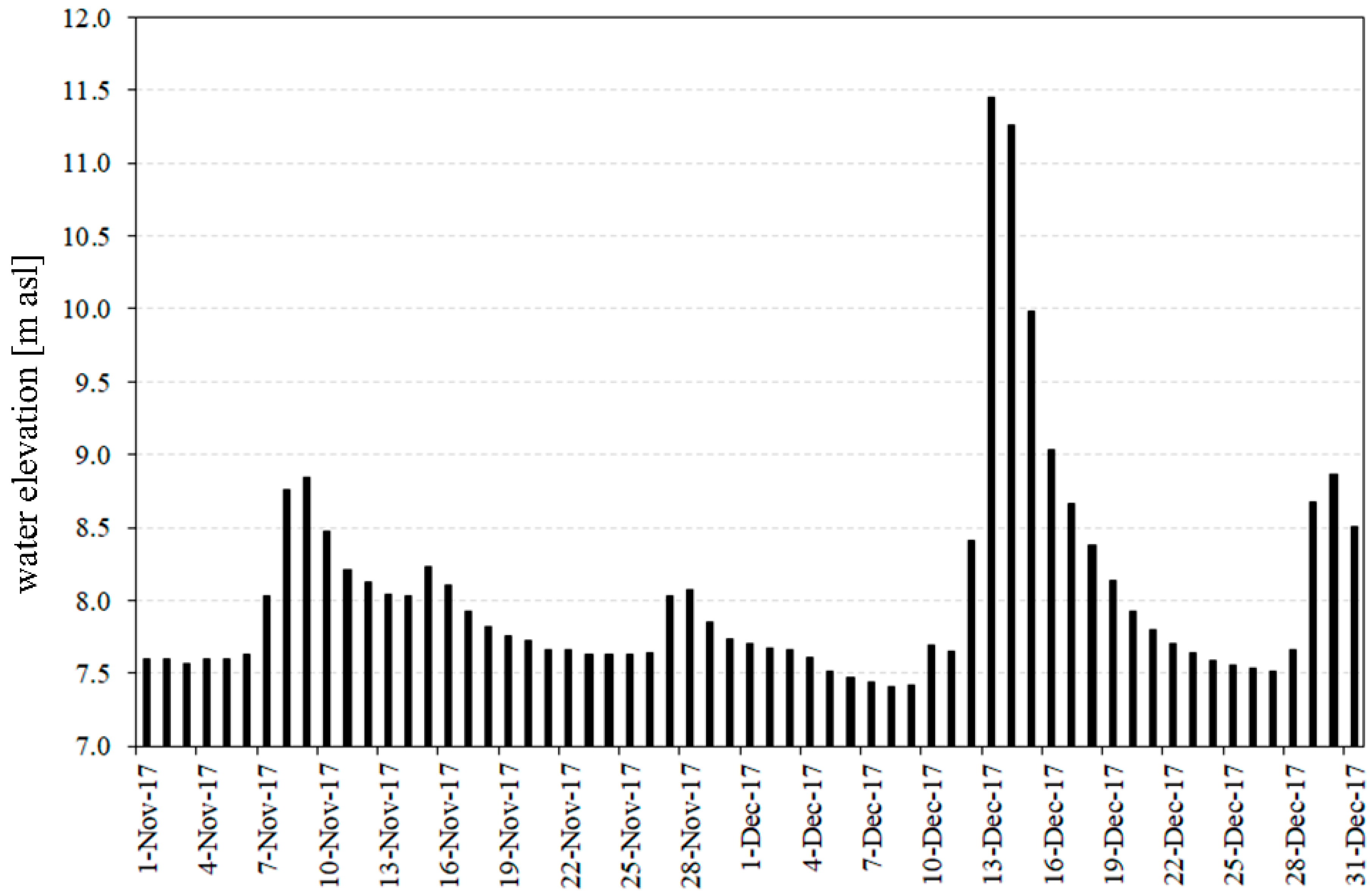
3.3. Water Level Data

The water levels were continuously monitored at the road bridge of Revere (coordinates 45°03′18″ N, 11°08′03″ E) located around 300 m upstream of the study area, where a gauging station measures the levels via a radar device. The data were acquired every 30 min, and an hourly average was adopted for the study case to give the level corresponding to edge-of-water lines tracked from 12-h spaced images. The water level at the gauging station was corrected based on the observed water slope along the river, eventually assessing the edge-of-water lines actual levels.

The reliability of the time-lapse photography in capturing the edge-of-water line changes of the sandbar was tested on the flooding event occurred in the period November–December 2017. As shown in Figure 4, increased precipitation started on 12 December, causing a flood wave in the region, which lasts for a couple days with significant values if compared to the typical low water depths measured before and after such event.

3.4. Model Implementation

To numerically model the flooding event with the iRIC 3.0 code, the domain was schematized using nested unstructured grids having a triangular shape, based on a previous analysis of the hydro-morphodynamics of the entire reach performed with the same solver [26]. As shown in Figure 5, for the entire domain, a maximum surface of 1000 m² for each cell was adopted, while between the two bridges, a finer grid of 250 m²/cell of maximum area was implemented. Aiming to describe in detail the morphodynamic evolution of the sandbar downstream of the railway bridge and the observed displacements of few meters, this area was discretized using a very fine grid of 50 m²/cell. Given these spatial constrictions, a sensitivity analysis on the numerical stability was performed, and for the runs, a time step of 0.2 s was eventually adopted, driving to relevant computational times for a standard PC with Intel Core i5.

The measured time series of water levels at Revere fixed the water depths in the model domain, whereas the flow velocities were computed by assuming a fixed bed roughness and water slope of 0.035 m^1/3/s and 7 × 10⁻⁵, respectively. This embeds a negligible loss of the hydraulic head that appears reasonable for the small domain simulated and aiming to reproduce the morphodynamics tendency for a very short period. Coherently with this approach, the incoming loads of sediment into the model domain were assumed in equilibrium with the hydraulic conditions and the river morphology at the boundary.

4. Results

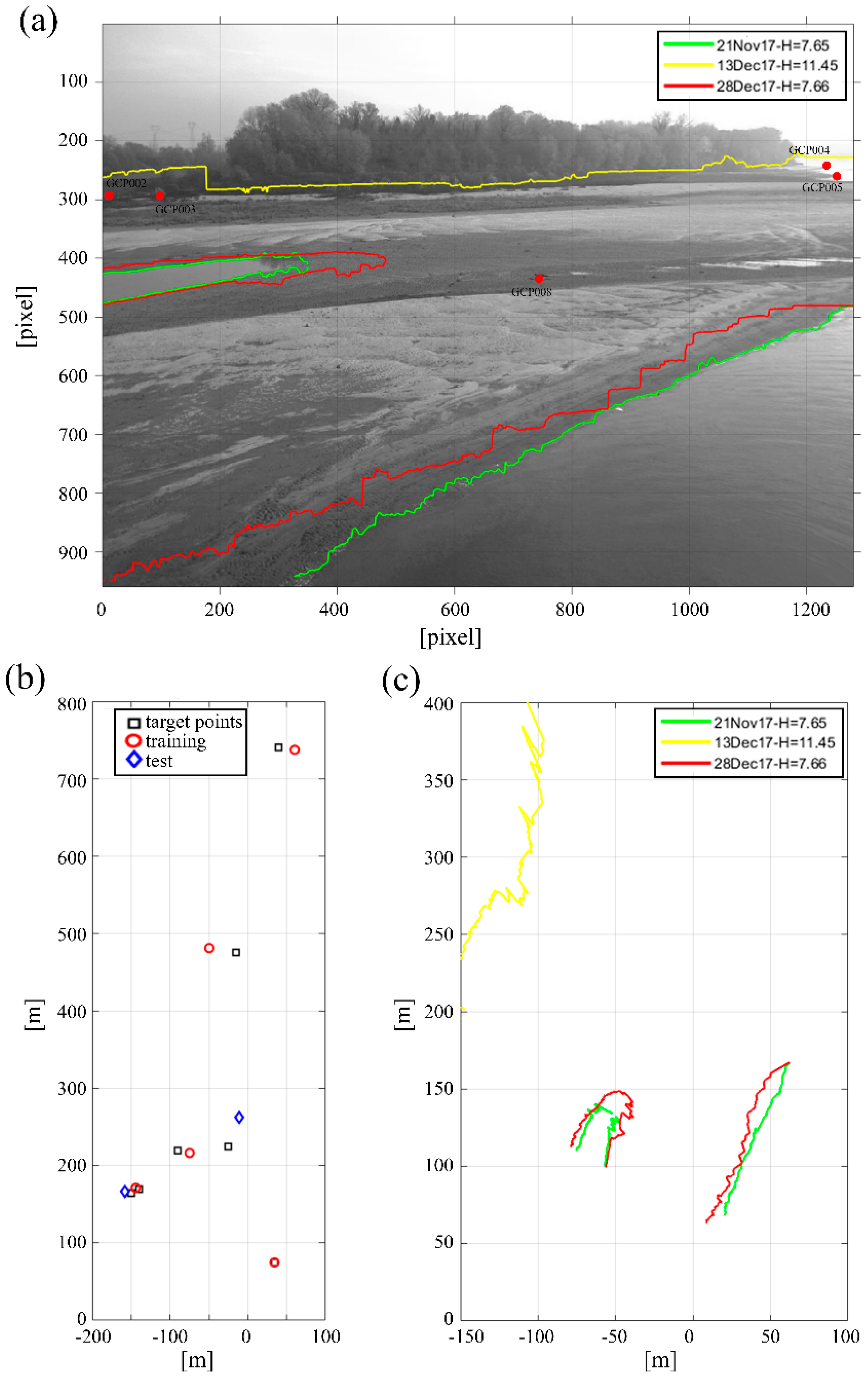
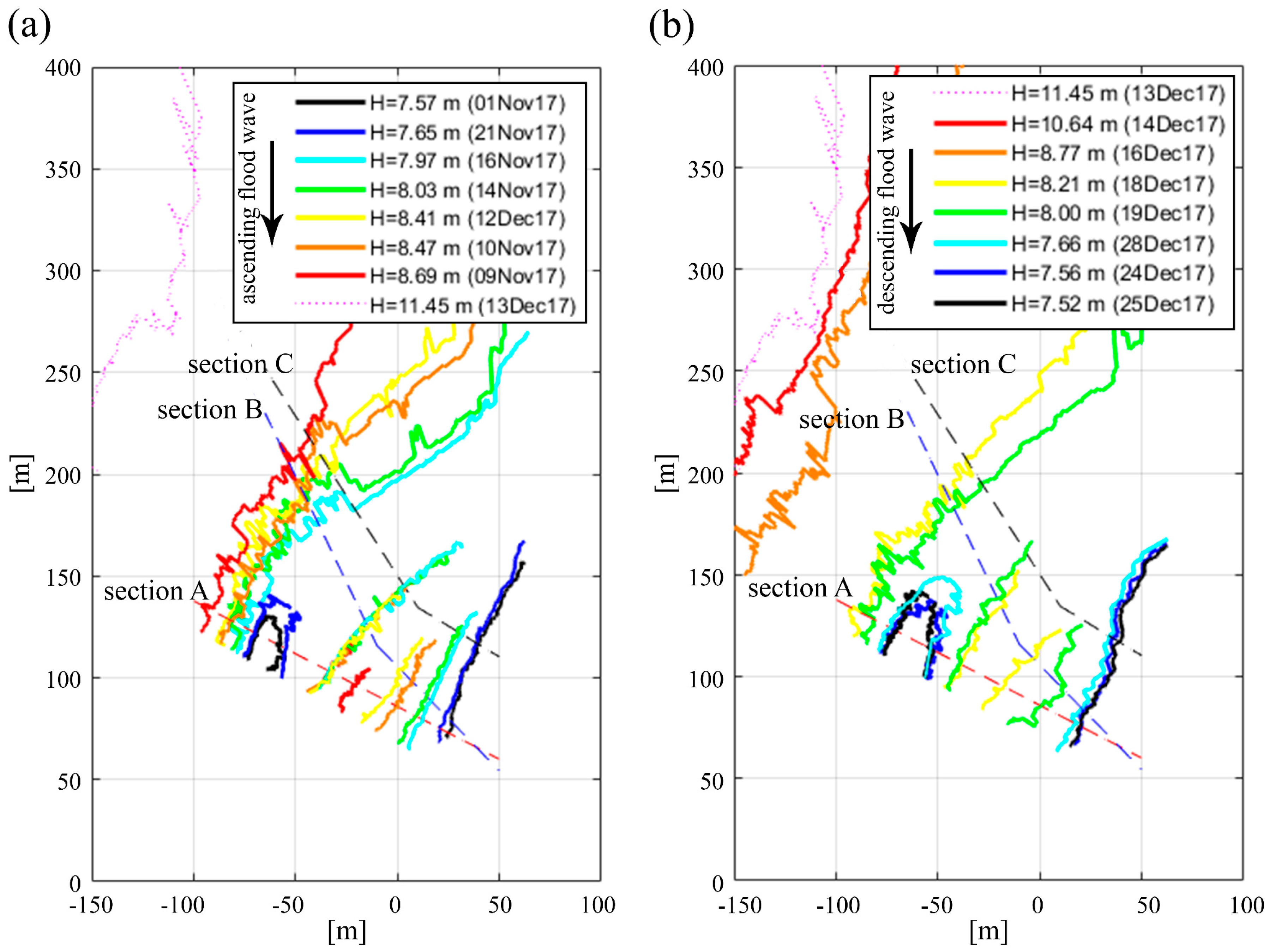
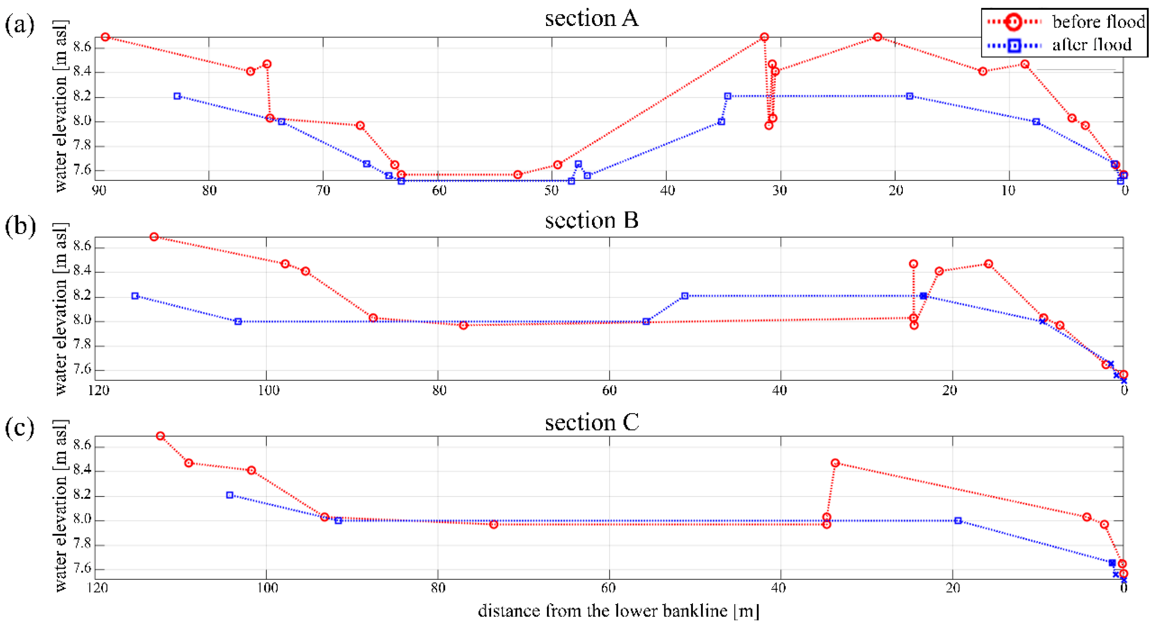
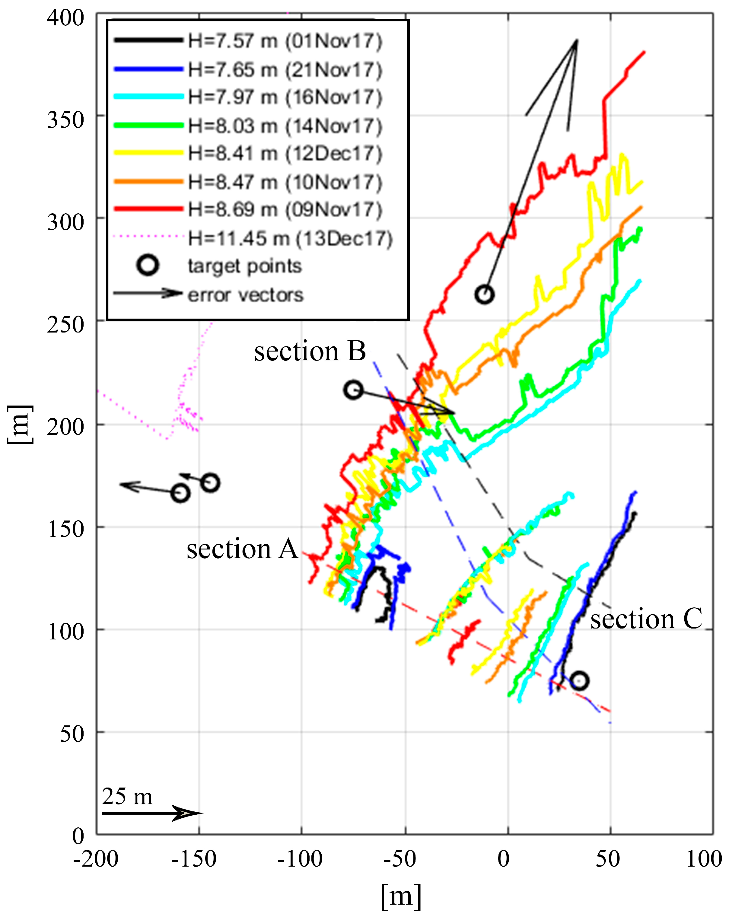
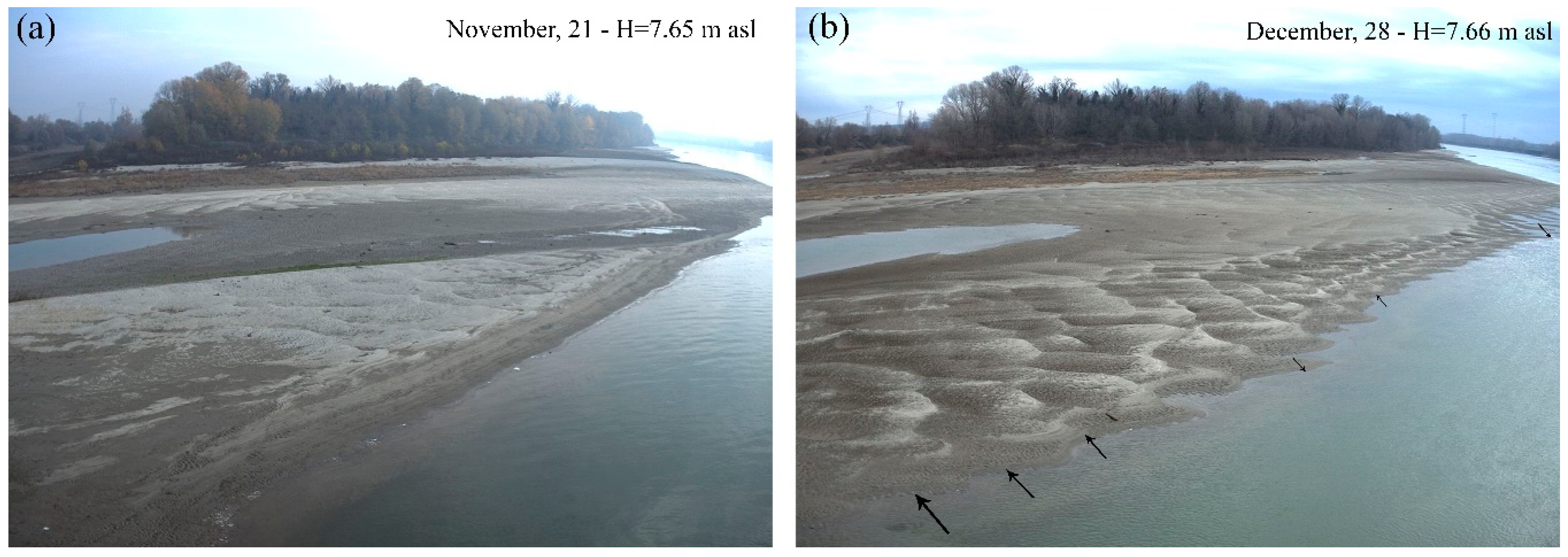
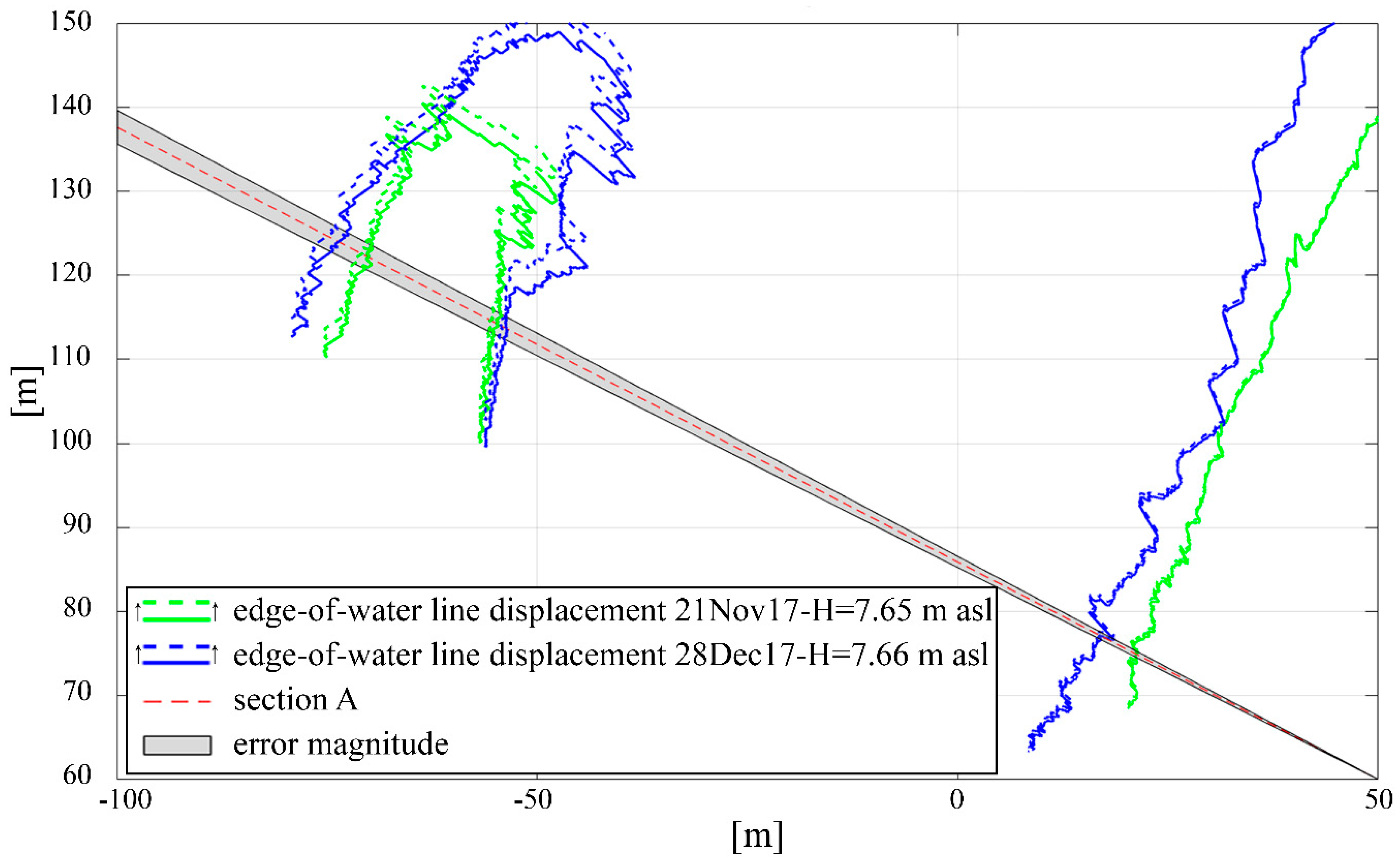
4.1. Edge-of-Water Line Evolution Monitored with the Camera

Several edge-of-water lines spanning the period November–December 2017 were tracked to evaluate the effects of a transient hydrology (flood wave) on the river morphology, namely the timeframe before and after the flooding event of 13 December. In comparing two images referred to the same water level (Figure 6), no specific bedforms were visible, but sediment movements are recognizable because of the flooding event (indicated here by the arrows). A quantitative estimation is not possible analyzing the raw data because of the image distortion and the absence of georeferenced information.

On the contrary, a quantitative estimation is possible based on the rectified images before and after the flood (Figure 7a,b, respectively). The evaluation of the riverbed changes was made on three cross-sections (namely, A, B and C in Figure 7), moving from close to the bridge towards downstream, and considering only the edge-of-water lines before and after the flood, neglecting the data referred to 13, 14 and 16 December that correspond to the peak levels.

As shown, section A is straight and closest to the camera, resulting in the shorter section, while the other two farther sections are longer (sections B and C). Section B intersects a variety of edge-of-water lines at the sandbar, corresponding to 5–7 water stages, while section C represents the downstream margin of the same bar. Based on these three cross sections, for each edge-of-water line, an intersection point was identified to reconstruct the river bottom profiles. The detected edge-of-water lines indicate a shallow area at the left margin of the thalweg, corresponding to the pier just next to the camera one. Even shallower at the left side, the Boschina Island is a rather stable zone as recognizable by the presence of well-established vegetation.

The river morphology is described in Figure 8, where the comparison between the cross sections A, B and C before and after the flooding event is reported. For all the analyzed cross-sections, an erosion is recognizable, indicating that the flood wave moved sediments towards downstream, with a higher magnitude close to the bridge (section A) rather than in the farther region (section C) because of the effect of the bridge piers. This comparison shows an erosion of the observed sandbar close to bridge piers, which protrudes for several meters downstream.

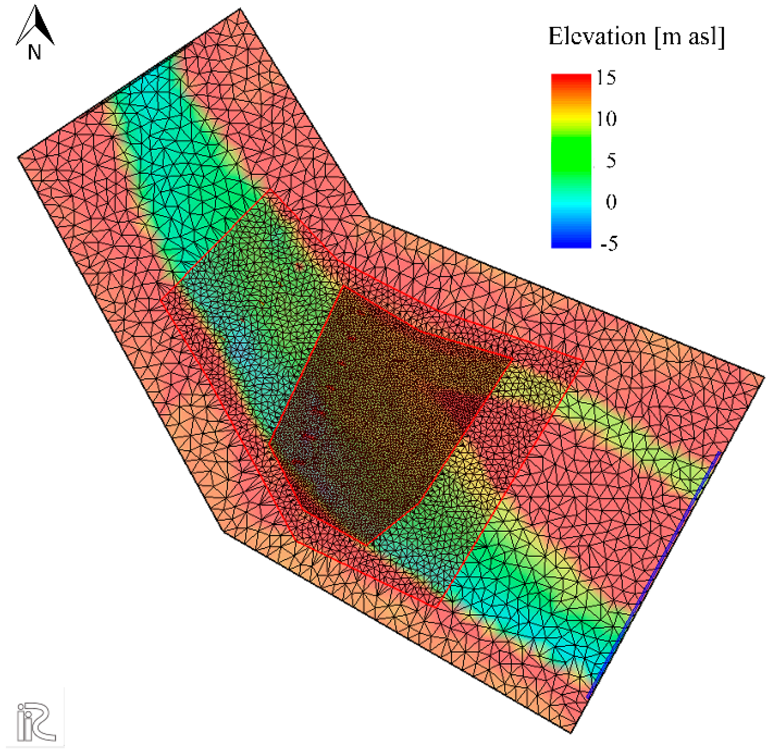
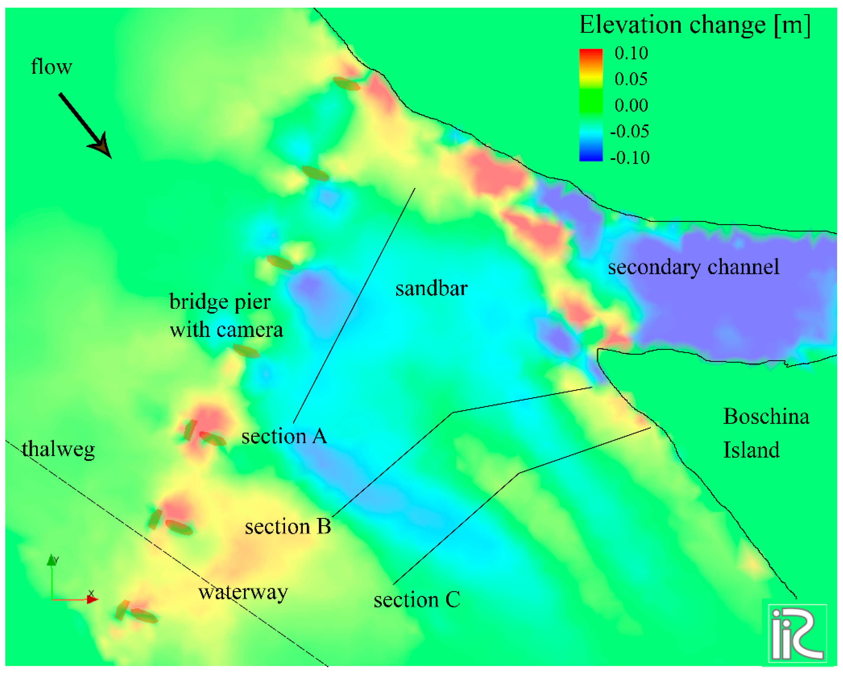
4.2. Modeled Evolution of the River Bed

The numerical modeling of this reach of the Po River provided a qualitative comparison with the morphological change derived from the time-lapse photography of the edge-of-water line displacements. In fact, the iRIC 3.0 suite along with its 2-D solver Mlow_02, was applied to simulate the flood of November–December 2017 by imposing the corresponding hydrograph measured at the Revere gauging station and using the DEM (Digital Elevation Model) derived from the ADCP survey of October 2017 combined with the 2005 2-m DEM as starting bathymetry.

After a preliminary calibration of the submerged (active) channel performed with the same code [26], several runs were carried out to analyze the capability of the model in reproducing the morphological change of the region submerged only during high flow conditions as observed from the time-lapse photography. The simulation outcomes show that increased velocities during the flooding event resulted in erosional patterns just downstream of the bridge piers. These regions correspond to the shallow area and the sandbar at the left side of the river channel, outside of the waterway (Figure 9). At the same time, a small deposition was simulated along the thalweg close to the right margin. The secondary channel on the left side, which creates the Boschina Island, appears with a noticeable deposition at its entrance that reduces the sediment incoming and causes the consequent degradation of the channel bed because of the outcome of sediments and water from downstream, corroborating field evidence.

The three piers located across the navigation channel (i.e., at the thalweg on the right side of the river channel) are characterized by protecting structures from floating debris and vessel impacts. These piers resulted in a deposition in the order of 5–10 cm, which is mainly due to the flow deceleration. On the contrary, the piers located on the left side of the river channel are poorly impacted by the main current, especially during normal base flow conditions but result with modest erosions after the flooding event.

Both the time-lapse photography and the numerical model point out a moderate erosion at the shallow area in the left side of the river channel that corresponds to a downstream displacement of the sandbar covering this shallow zone. The erosion is assessed in the order of tens of centimeters from the edge-of-water lines detection performed with the camera, while the iRIC model simulates variations of few centimeters because of the constraints related to such kind of modeling.

5. Discussion

The photogrammetric method requires a calibration of the camera parameters (lens distortion, focus, etc.) and on the positioning of the target points to adequately transpose the image coordinates into the real-world ones. As described in Section 2.2, the transposition from image to real-world coordinates was performed using a linear homography calibrated and validated with seven target points obtained from a DGPS survey and satellite imagery. Given the reduced number of points and the simple relationship chosen, this operation introduces errors in the planimetric positions of the image portions, which are evaluated by subtracting the actual positions of the target points from the assessed ones (arrows in Figure 10, double-scaled to improve the readability). These errors are rather irrelevant close to the camera, but can reach tens of meters in the very far-field. However, for the evaluated cross-sections (section A, B and C in Figure 10) close to the camera, such errors have a quite low influence, having the same order of magnitude of the image resolution and resulting in few meters of displacement of the tracked edge-of-water lines.

An error analysis was performed focusing on section A, which is the closest to the bridge pier. In this case, the positioning errors range from 5–10 cm along the lower edge-of-water line (low-right angle in Figure 10) to around 4 m for the edge-of-water lines detected close to the Boschina Island (end of section A on the left side). Given the low number of target points, a linear variation of the error while moving along the section A is assumed (i.e., error changes in the range 0.1–4 m). The edge-of-water lines displacement is reconstructed as influenced by the observed errors in the homographic projection (Figure 11) to estimate the deviation between the positions of the actual and the projected edge-of-water lines. As visible, this deviation is not significantly close to the camera and can be estimated in few meters for the edge-of-water lines located further away from the bridge pier. However, given the large length and small slope of the observed sandbar (i.e., 300–400 m and 1–5%, respectively), a deviation of few meters in the horizontal plan appears negligible and does not reflect in a significant variation in the corresponding bed elevation. In addition, the difference between the reconstructed morphologies before and after the flooding event is only slightly affected by the errors in the edge-of-water lines positioning. As a matter of fact, these errors are comparable at a given distance from the camera and therefore they reduce the edge-of-water lines differences.

The numerical modeling bears out a river section redistribution during a flood: the thalweg at the right side is slightly deposited whereas the sandbar close to the Boschina Island is eroded. This is consistent with the observed changes of the bar morphology from the time-lapse photography and prove the expected succession of the river channel narrowing and widening during dry and flood seasons, respectively. Despite this agreement among video analysis and the numerical model, the latter clearly underestimate the bar erosion during the flood. As a matter of fact, the simulated erosion is few centimeters rather than in the order of 10⁻¹ m as it results from the time-lapse photography and previous research [32,43], although other application of the same model [26] shown that it can represent the overall dynamics of this reach. The underestimation can be ascribed to the limited length of the computation domain, the adopted sediment transport equations and to the imposed conditions of equilibrium between water and flow discharges at the model boundaries, that make persistent the initial morphology. These limitations are particularly relevant for the simulation of the dynamics of the emerged bar, which have a wavelength in the order of the computational domain length. In addition, the model runs were performed based on a fixed roughness (Manning coefficient n = 0.035 m^1/3/s) for the entire channel, that reproduces quite well the active channel dynamics [26] but, as observable here, this schematization could be not adequate to evaluate the sudden changes on temporarily dry regions.

Despite the differences in simulating the sandbar changes, the qualitative comparison between time-lapse photography and modeling results highlights the importance of using continuous video monitoring to be further applied for the calibration of existing numerical modeling tools. In particular, this camera-based method captured the dynamics of the emerged sandbars along the Po River that clearly indicate the need for a specific implementation in a CFD model to properly represent the sandbar dynamics.

To overcome the usual limitation of available field data regarding the emerged parts of a river, the monitoring of edge-of-water line displacements with noninvasive techniques like the photogrammetric method described here can be very helpful. As a matter of fact, once installed, the camera can acquire images for very long periods, covering all the water level conditions and therefore evaluating the long-term morphodynamics of the watercourse. The morphological changes of large sandy rivers are quite slow and can be satisfactorily tracked via edge-of-water line monitoring with long timeframes.

A traditional survey of the river morphology uses the DGPS, which measures the landscape evolution in a very precise manner, reaching the accuracy of within a few centimeters—both in planimetry and altimetry. Besides the initial costs of the instrumentation, however, the surveying of the evolution of a riverine environment for long periods (i.e., 5–10 years depending on the hydromorphological and sedimentological conditions) to eventually evaluate the fluvial morphodynamics appears costly also in terms of human workforce. As an example, to acquire the ground control points and dynamically track one edge-of-water line in the Po River case study, two persons work for half a day. In first approximation, one can estimate that this DGPS campaign should be repeated around four times per year given the typical hydrological cycle (two peaks in discharge, generally in autumn and spring) to adequately track the consequent morphological changes. On the contrary, the use of fixed cameras operating remotely are more profitable, both from a purely economic point of view and considering the workforce required. Indeed, if the initial costs of the instrumentation (i.e., camera and acquisition system versus DGPS) may be comparable, the camera operates autonomously once installed, possibly requiring some sporadic maintenance and only one field campaign to adequately calibrate the system. In the long-term, this contributes to reduce the management costs in favor of a cheap, continuous and reliable, although less accurate, representation of the river morphodynamics. Indeed, aiming to reproduce the edge-of-water line dynamics of semi-exposed regions of sandy river, an accuracy of some meters in the planimetric positioning may be enough, while coupling the planimetric view from photogrammetry with water elevation acquired via a radar system assures an altimetric accuracy of few centimeters, comparable with the one of a traditional DGPS. This accuracy is appropriate to track large sandbars dynamic driven by flood events as in the case study presented herein.

To improve the planimetric accuracy of the edge-of-water line displacements extracted from images analysis, a detailed calibration should be performed, using several target points equally distributed in the entire field view. As for the present case study, in fact, one of the constraints is that it was not possible to cover all the calibration imaged with points acquired with a DGPS given the presence of water on the right side and trees on the background. To overcome such a limitation and increase the database of ground control points, satellite images were analyzed, eventually yielding additional points but with a lower accuracy. For the future, specific field campaigns using Unmanned Surface Vehicles (USV) are planned to complete the dataset of target points that will improve the calibration and therefore reduce the planimetric errors observed in this preliminary application.

In addition, the present study proves the advantages of a video camera method in tracking edge-of-water line displacements with respect to more established methods like satellite imagery and on-the-fly techniques [49,50]. Indeed, Landsat and Sentinel sensors have a resolution of 30 m and 10 m, respectively, which is one order of magnitude higher than the time-lapse photography accuracy, once calibrated with well-distributed target points. Even more relevant, the temporal resolution is clearly in favor of the camera, given that satellites images are available every 15–30 days, and therefore cannot be used to track relatively fast phenomena like flood waves. Moreover, having a comparable resolution of the obtained images [51,52], the use of a fixed camera could overcome some limitations related to using unmanned aerial vehicles (UAV) in nonoptimal weather conditions, which are likely to happen during floods, being complementary to largely adopted methods [53,54].

Positional uncertainties (namely, the uncertainty in both the horizontal and the vertical location of individual topographic points in a point cloud) are the main source of errors for such kind of measurements [50]. The sources of positional uncertainties are the sensor’s precision and accuracy, the geometry of acquisition and the position of the sensor [55]. Requiring a field campaign with DGPS, uncertainties associated with time-lapse photography are a combination of precision and accuracy of the used GPS system (centimeters) and the resolution of the captured images (around one meter).

The use of economic and noninvasive techniques for monitoring river at the long-term can result fundamental in water management, addressing one of the major problems of river restoration: the project age [56]. Indeed, post-project monitoring is one of the missing gaps in fluvial restoration because of its costs and technical challenges, and the proposed approach via edge-of-water line tracking can overcome these problems in a relatively profitable manner. Moreover, besides the evaluation of the river morphodynamics, the present approach can be further developed to dynamically track the riparian vegetation, to eventually derive metrics helpful in assessing the overall quality of a watercourse.

6. Conclusions

Aiming to investigate the sandbar dynamics and the consequent variations of the riverbed, a simple video-based method was applied, which continuously acquired the edge-of-water line positions of a large and semiexposed sandbar in the Po River in Italy. The occurred morphological change is therefore evaluated and qualitatively compared to numerical modeling results. The quantification this change is achieved through the mapping of multiple edge-of-water lines of the sandbar by using a fixed camera for the planimetric positioning and the recording from a nearby hydrological gauging station giving the corresponding water levels. Both the time-lapse photography and numerical results show that, in this region, flood waves can easily remove sediments that accumulated at bars during low flow conditions. In fact, the flooding event redistributes the river flow into a wider cross section, reshaping the deepening and narrowing of the main channel typically observed during dry periods and described by previous studies.

The paper demonstrates that monitoring the riverine edge-of-water line displacements with a fixed camera can be an economical and reliable method for reproducing the river morphodynamics by detecting the changes of emerged morphological features due to flooding happenings, thus offering novel evidence for numerical models’ calibration. This preliminary application shows the feasibility of the proposed approach and suggests its application to larger periods to simulate the long-term evolution of alluvial rivers with a higher resolution with respect to satellite imagery, requiring a limited effort in terms of workforce.

References

1. Marion, A.; Nikora, V.; Puijalon, S.; Bouma, T.; Koll, K.; Ballio, F.; Tait, S.; Zaramella, M.; Sukhodolov, A.; O’Hare, M.T.; et al. Aquatic interfaces: A hydrodynamic and ecological perspective. J. Hydraul. Res. 2014, 52, 744–758. [Google Scholar] [CrossRef]
2. Gurnell, A.M.; Corenblit, D.; García de Jalón, D.; González del Tánago, M.; Grabowski, R.C.; O’Hare, M.T.; Szewczyk, M. A Conceptual Model of Vegetation–hydrogeomorphology Interactions within River Corridors. River Res. Appl. 2016, 32, 142–163. [Google Scholar] [CrossRef]
3. Nones, M.; Di Silvio, G. Modeling of River Width Variations Based on Hydrological, Morphological, and Biological Dynamics. J. Hydraul. Eng. 2016, 142, 04016012. [Google Scholar] [CrossRef]
4. Vesipa, R.; Camporeale, C.; Ridolfi, L. Effect of river flow fluctuations on riparian vegetation dynamics: Processes and models. Adv. Water Resour. 2017, 110, 29–50. [Google Scholar] [CrossRef]
5. Scorpio, V.; Zen, S.; Bertoldi, W.; Surian, N.; Mastronunzio, M.; Dai Prà, E.; Zolezzi, G.; Comiti, F. Channelization of a large Alpine river: What is left of its original morphodynamics? Earth Surf. Process. Landf. 2018, 43, 1044–1062. [Google Scholar] [CrossRef]
6. Amitrano, D.; Di Martino, G.; Iodice, A.; Riccio, D.; Ruello, G.; Ciervo, F.; Papa, M.N.; Koussoubè, Y. Effectiveness of high-resolution SAR for water resource management in low-income semi-arid countries. Int. J. Remote Sens. 2014, 35, 70–88. [Google Scholar] [CrossRef]
7. Domeneghetti, A. On the use of SRTM and altimetry data for flood modeling in data-sparse regions. Water Resour. Res. 2016, 52, 2901–2918. [Google Scholar] [CrossRef]
8. Payne, C.; Panda, S.; Prakash, A. Remote Sensing of River Erosion on the Colville River, North Slope Alaska. Remote Sens. 2018, 10, 397. [Google Scholar] [CrossRef]
9. Schwenk, J.; Khandelwal, A.; Fratkin, M.; Kumar, V.; Foufoula-Georgiou, E. High spatiotemporal resolution of river planform dynamics from Landsat: The RivMAP toolbox and results from the Ucayali River. Earth Space Sci. 2017, 4, 46–75. [Google Scholar] [CrossRef]
10. Moretto, J.; Rigon, E.; Mao, L.; Picco, L.; Delai, F.; Lenzi, M.A. Channel adjustments and island dynamics in the Brenta River (Italy) over the last 30 years. River Res. Appl. 2014, 30, 719–732. [Google Scholar] [CrossRef]
11. Nones, M.; Gerstgraser, C. Morphological changes of a restored reach: The case of the Spree River, Cottbus, Germany. In Hydrodynamic and Mass Transport at Freshwater Aquatic Interfaces, 167–182 GeoPlanet: Earth and Planetary Sciences; Rowiński, P., Marion, A., Eds.; Springer International Publishing: Cham, Switzerland, 2016. [Google Scholar]
12. Spiekermann, R.; Betts, H.; Dymond, J.; Basher, L. Volumetric measurement of river bank erosion from sequential historical aerial photography. Geomorphology 2017, 296, 193–208. [Google Scholar] [CrossRef]
13. Langhammer, J.; Bernsteinová, J.; Miřijovský, J. Building a High-Precision 2D Hydrodynamic Flood Model Using UAV Photogrammetry and Sensor Network Monitoring. Water 2017, 9, 861. [Google Scholar] [CrossRef]
14. Micheletti, N.; Chandler, J.H.; Lane, S.N. Investigating the geomorphological potential of freely available and accessible structure-from-motion photogrammetry using a smartphone. Earth Surf. Process. Landf. 2015, 40, 473–486. [Google Scholar] [CrossRef] [Green Version]
15. Archetti, R.; Paci, A.; Carniel, S.; Bonaldo, D. Optimal index related to the shoreline dynamics during a storm: The case of Jesolo beach. Nat. Hazards Earth Syst. Sci. 2016, 16, 1107–1122. [Google Scholar] [CrossRef]
16. Pyle, C.J.; Richards, K.S.; Chandler, J.H. Digital photogrammetric monitoring of river bank erosion. Photogramm. Rec. 1997, 15, 753–764. [Google Scholar] [CrossRef]
17. Chandler, J.H. Effective application of automated digital photogrammetry for geomorphological research. Earth Surf. Process. Landf. 1999, 24, 51–63. [Google Scholar] [CrossRef]
18. Stojic, M.; Chandler, J.H.; Ashmore, P.; Luce, J. The assessment of sediment transport rates by automated digital photogrammetry. Photogramm. Eng. Remote Sens. 1998, 64, 387–395. [Google Scholar]
19. Aarninkhof, S.G.J.; Turner, I.L.; Dronkers, T.D.T.; Caljouw, M.; Nipius, L. A video-based technique for mapping intertidal beach bathymetry. Coast. Eng. 2003, 49, 275–289. [Google Scholar] [CrossRef]
20. Kroon, A.; Davidson, M.A.; Aarninkhof, S.G.J.; Archetti, R.; Armaroli, C.; Gonzalez, M.; Medri, S.; Osorio, A.; Aagaard, T.; Holman, R.A.; et al. Application of remote sensing video systems for coastline management problems. Coast. Eng. 2007, 54, 493–505. [Google Scholar] [CrossRef]
21. Archetti, R. Quantifying the evolution of a beach protected by low crested structures using video monitoring. J. Coast. Res. 2009, 25, 884–899. [Google Scholar] [CrossRef]
22. Archetti, R.; Romagnoli, C. Analysis of the effects of different storm events on shoreline dynamics of an artificially embayed beach. Earth Surf. Process. Landf. 2011, 36, 1449–1463. [Google Scholar] [CrossRef]
23. Archetti, R.; Zanuttigh, B. Integrated monitoring of the hydro-morphodynamics of a beach protected by low crested detached breakwaters. Coast. Eng. 2010, 57, 879–891. [Google Scholar] [CrossRef]
24. Domeneghetti, A.; Carisi, F.; Castellarin, A.; Brath, A. Evolution of flood risk over large areas: Quantitative assessment for the Po River. J. Hydrol. 2015, 527, 809–823. [Google Scholar] [CrossRef]
25. Schumann, G.J.-P.; Domeneghetti, A. Exploiting the proliferation of current and future satellite observations of rivers. Hydrol. Process. 2016, 30, 2891–2896. [Google Scholar] [CrossRef]
26. Nones, M.; Pugliese, A.; Domeneghetti, A.; Guerrero, M. Po River morphodynamics modelled with the open-source code iRIC. In Free Surface Flows and Transport Processes. GeoPlanet: Earth and Planetary Sciences; Kalinowska, M., Mrokowska, M., Rowiński, P., Eds.; Springer: Cham, Switzerland, 2018. [Google Scholar]
27. Amorosi, A.; Maselli, V.; Trincardi, F. Onshore to offshore anatomy of a late Quaternary source-to-sink system (Po Plain-Adriatic Sea, Italy). Earth-Sci. Rev. 2016, 153, 212–237. [Google Scholar] [CrossRef]
28. Syvitski, J.P.M.; Kettner, A.J. On the flux of water and sediment into the Northern Adriatic Sea. Cont. Shelf Res. 2007, 27, 296–308. [Google Scholar] [CrossRef]
29. Cozzi, S.; Giani, M. River water and nutrient discharge in the Northern Adriatic Sea: Current importance and long-term changes. Cont. Shelf Res. 2011, 31, 1881–1893. [Google Scholar] [CrossRef]
30. Montanari, A. Hydrology of the Po River: Looking for changing patterns in river discharge. Hydrol. Earth Syst. Sci. 2012, 16, 3739–3747. [Google Scholar] [CrossRef]
31. Cati, L. Idrografia e Idrologia del Po; Ufficio Idrografico del Po: Parma, Italy, 1981. (In Italian) [Google Scholar]
32. Guerrero, M.; Lamberti, A. Flow Field and Morphology Mapping Using ADCP and Multibeam Techniques: Survey in the Po River. J. Hydraul. Eng. 2011, 137. [Google Scholar] [CrossRef]
33. Lamberti, A.; Schippa, L. Studio dell’abbassamento del fiume Po: Previsioni trentennali di abbassamento a Cremona. In Navigazione Interna; Azienda Regionale per i Porti di Cremona e Mantova: Cremona, Italy, 1994. (In Italian) [Google Scholar]
34. Lanzoni, S. Evoluzione morfologica recente dell’asta principale del Po. In Proceedings of the Convegni dei Lincei; Giornata Mondiale dell’Acqua, Accademia Nazionale dei Lincei: Roma, Italy, 2012. (In Italian) [Google Scholar]
35. Surian, N.; Rinaldi, M. Morphological response to river engineering and management in alluvial channels in Italy. Geomorphology 2003, 50, 307–326. [Google Scholar] [CrossRef]
36. Zanchini, F. Metodi di Rilievo degli Argini Mediante Utilizzo di Tecniche Geomatiche Integrate: Isola Boschina, Ostiglia, Mantova. Master’s Thesis, University of Bologna, Italy, 2017. (In Italian). [Google Scholar]
37. Astori, B.; Solaini, L. Fotogrammetria. Clup: Milano, Italy, 1974. (In Italian) [Google Scholar]
38. Guerrero, M.; Lamberti, A. Clouds image processing for velocity acquisition. In Proceedings of the 32nd IAHR Congress, Venice, Italy, 1–6 July 2007. [Google Scholar]
39. Nelson, J.M.; Shimizu, Y.; Abe, T.; Asahi, K.; Gamou, M.; Inoue, T.; Iwasaki, T.; Kakinuma, T.; Kawamura, S.; Kimura, I.; et al. The international river interface cooperative: Public domain flow and morphodynamics software for education and applications. Adv. Water Resour. 2016, 93, 62–74. [Google Scholar] [CrossRef]
40. iRIC Software. Mflow_02 Solver Manuals. 2014. Available online: http://i-ric.org (accessed on 8 May 2018).
41. Nezu, I.; Nakagawa, H. Turbulence in Open-Channel Flow; IAHR Monograph, Belkema: Rotterdam, The Netherlands, 1993. [Google Scholar]
42. Lomax, H.; Pulliam, T.H.; Zingg, D.W. Fundamentals of Computational Fluid Dynamics; Springer: Berlin/Heidelberg, Germany, 2013. [Google Scholar]
43. Guerrero, M.; Di Federico, V.; Lamberti, A. Calibration of a 2-D morphodynamic model using water–sediment flux maps derived from an ADCP recording. J. Hydroinform. 2013, 15, 813–828. [Google Scholar] [CrossRef]
44. Ashida, K.; Michiue, M. Studies on Bed Load Transportation for Nonuniform Sediment and River Bed Variation; Disaster Prevention Research Institute Annuals: Kyoto, Japan, 1972; 14p. [Google Scholar]
45. Garcia, M.H.; Parker, G. Entrainment of bed sediment into suspension. J. Hydraul. Eng. 1991, 144, 414–435. [Google Scholar] [CrossRef]
46. Rouse, H. Modern conception of the mechanics of turbulence. Trans. ASCE 1937, 102, 463–543. [Google Scholar]
47. Agenzia Interregionale per il Fiume Po—AIPO. Rilievo Sezioni Topografiche Trasversali Nella Fascia B del Fiume Po, Dalla Confluenza con il Ticino al Mare; AIPO: Parma, Italy, 2005. (In Italian) [Google Scholar]
48. Nones, M.; Guerrero, M.; Conevski, S.; Rüther, N.; Di Federico, V. The acoustic backscatter at two well-spaced grazing angles to characterize moving sediments at riverbed. In Proceedings of the XXXVI Convegno Nazionale di Idraulica e Costruzioni Idrauliche, Ancona, Italy, 12–14 September 2018. [Google Scholar]
49. Donchyts, G.; Baart, F.; Winsemius, H.; Gorelick, N.; Kwadijk, J.; van de Giesen, N. Earth’s surface water change over the past 30 years. Nat. Clim. Chang. 2016, 6, 810–813. [Google Scholar] [CrossRef]
50. Passalacqua, P.; Belmont, P.; Staley, D.M.; Simley, J.D.; Arrowsmith, J.R.; Bode, C.A.; Crosby, C.; DeLong, S.B.; Glenn, N.F.; Kelly, S.A.; et al. Analyzing high resolution topography for advancing the understanding of mass and energy transfer through landscapes: A review. Earth-Sci. Rev. 2015, 148, 174–193. [Google Scholar] [CrossRef] [Green Version]
51. Rusnák, M.; Sládek, J.; Kidová, A.; Lehotský, M. Template for high-resolution river landscape mapping using UAV technology. Measurement 2018, 115, 139–151. [Google Scholar] [CrossRef]
52. Legleiter, C.J.; Roberts, D.A.; Lawrence, R.L. Spectrally based remote sensing of river bathymetry. Earth Surf. Process. Landf. 2009, 34, 1039–1059. [Google Scholar] [CrossRef]
53. Legleiter, C.J. Remote measurement of river morphology via fusion of LiDAR topography and spectrally based bathymetry. Earth Surf. Process. Landf. 2012, 37, 499–518. [Google Scholar] [CrossRef]
54. Kelly, S.A.; Belmont, P. High Resolution Monitoring of River Bluff Erosion Reveals Failure Mechanisms and Geomorphically Effective Flows. Water 2018, 10, 394. [Google Scholar] [CrossRef]
55. Lichti, D.D.; Skaloud, J. Registration and calibration. In Airborne and Terrestrial Laser Scanning; Vosselman, G., Maas, H.-G., Eds.; CRC Press Inc.: Boca Raton, FL, USA, 2010; pp. 83–133. [Google Scholar]
56. Nones, M. River restoration: The need for a better monitoring agenda. In Proceedings of the 13th International Symposium on River Sedimentation, Stuttgart, Germany, 19–22 September 2016; pp. 908–913. [Google Scholar]
Figure 1. Study site: (a) Po River catchment; (b) satellite image; (c) digital elevation model of the studied reach close to the city of Revere; (d) location of the camera on the railway bridge crossing the Po River at Revere (sight from downstream).
Water 10 00617 g001
Figure 2. (a) Example of edge-of-water line tracking on the original image and location of some ground control points. (b) The two-steps method for the homographic transformation between image and real plane coordinates. (c) Example of corrected edge-of-water line positions.
Water 10 00617 g002
Figure 3. (a) Location of the camera and example of images acquired at Revere in (b) low flow conditions and (c) during the flooding event.
Water 10 00617 g003
Figure 4. Water levels measured at the Revere gauging station in the analyzed period of November–December 2017.
Water 10 00617 g004
Figure 5. Nested grid structure and elevation of the bottom.
Water 10 00617 g005
Figure 6. Images captured (a) before and (b) after the flooding event of December 13. The water levels are almost the same: on November 21 (a) it was 7.65 m a.s.l., while on December 28 (b) was 7.66 m a.s.l. The arrows indicate the displacement of the edge-of-water line.
Water 10 00617 g006
Figure 7. Riverine edge-of-water lines during the (a) ascending and (b) descending waves of the flooding event of December 13 (magenta pointed line). The dashed lines locate the three cross sections used to evaluate the morphological changes.
Water 10 00617 g007
Figure 8. Comparison between riverine morphologies before (red line) and after (blue line) the flooding event in (a) section A, (b) section B and (c) section C, as resulted from the edge-of-water lines time-lapse photography. The x-axis represents the distance from the lower edge-of-water line while the y-axis indicates the water elevation measured at the gauging station of Revere corrected by accounting for the mean slope of the free surface.
Water 10 00617 g008
Figure 9. Simulated erosion and deposition pattern numerically modeled with iRIC.
Water 10 00617 g009
Figure 10. Deviations between actual and calculated positions of target points from the homography reported on the edge-of-water lines map. Error arrows are double-scaled.
Water 10 00617 g010
Figure 11. Variation of the error magnitude along the section A and the estimated deviations between positions of actual and projected edge-of-water lines.
Water 10 00617 g011