Abstract
River systems are crucial for the Earth system. However, they are profoundly impacted by human activities, especially land use change. To reveal the impact of land use change on river systems, river system data and land use data in Suzhou City from the 1960s to 2010s were analyzed through grid river density on a 3 km × 3 km scale. The spatial-temporal variation was very different for different river orders. The lower the river order, the larger was the variation in the accumulated length (including both an increase and a decrease). The river systems were modified to meet the needs of human development in different social development stages. During the period of agricultural modification, undeveloped land was reclaimed to increase the amount of arable land available, but when the proportion of cultivated land exceeded a threshold level, higher order rivers were invaded, cut off and even buried, which forced a part of the higher order rivers to transform into narrower rivers. During the period of urbanization, higher order rivers were usually dredged, reconstructed and protected to improve the abilities of storage and discharge, and lower order rivers were buried after 40% of the land proportion had been built up. These results provide a reliable foundation on which to formulate policies and manage river systems.
1. Introduction
The surface landscape is often fundamentally altered during economic and social development, and quantity, morphology, and structure of river systems are usually inadvertently influenced along with land use change [1,2,3]. Strahler [4] initially outlined erosion and aggradation as system responses when a steady state was upset by human activities. Wolman [5] further revealed how river channels respond to three stages of urban development: an equilibrium pre-development stage; a period of construction during which bare land is exposed to erosion, leading to sedimentation within river channels; a stage of urban landscape that is dominated by an impervious surface, leading to increased runoff and decreased sediment production, followed by continued river channel erosion from increased runoff coupled with a decline in sediment that yield enlarged river channels. A compilation of research results from more than 100 studies all over the world found that persistence of the sediment production phase varied from months to several years, whereas several decades were likely needed for enlarging river channels to stabilize and potentially reach a new equilibrium [6]. The hydro-geomorphic response to land use change is further amplified when river systems are deliberately modified—to meet the needs of human development (e.g., agricultural modification, industrialization, urbanization)—through reshaping, widening, occupation and burial, etc. [7], and has been identified as one of the most widespread and dramatic influences on river systems since the middle of the twentieth century [1].
In Nurmijarvi (Southern Finland), the number and length of open ditches decreased by 88% (from 323 to 40) and 69% (from 97,896 m to 30,537 m), respectively—caused by agricultural modification from 1954 to 1997—and on average about 500 m/ha of open ditches have been replaced by subsurface drains over the state [8]. A similar phenomenon occurred in the Lake Thunderbird Watershed (Oklahoma, USA) where almost 25% of the river length was lost from 1942 to 2011; most river losses were replaced by agriculture. Furthermore, urban development has gradually increased river loss and disconnection [3]. As urban development has intensified, the size, shape, and connectivity of urban water bodies (rivers, lakes, wetlands and so on) are increasingly different from that of undeveloped landscapes, and surface water distribution in cities is more similar to each other than that of their surrounding landscapes. This phenomenon has been verified by comparing water bodies of 100 U.S. cities with their surrounding undeveloped land. The river density and water surface rate decreased by 71% and 89%, respectively, compared to that of undeveloped land; however, urbanization has increased the occurrence of surface water in drier landscapes [9]. A sharp decrease in river channels has led to an increase in the number of urban river deserts (i.e., areas within a watershed that exhibit no surface river channels due to the effects of human development and population growth) [7,10] and a heavy dependence on engineered subsurface water conveyance systems, creating what has been referred to as urban karst [11]. However, as time goes on, aging and poorly maintained underground pipes are no longer able to function, inflicting more pressure on the already reduced river systems.
As river systems have a fundamental role in the movement of organisms and dead matter [12], being an important carrier of water source, river channel and riparian zone [13], the status of river systems is closely related to water resources [14,15], the water environment [16], and the water ecosystem [8,17]. It is necessary to analyze the form and processes of river systems in the past, present, and future to reveal the interrelationship between the evolution of river systems and human activities, especially land use change [18]. This will allow us to learn and adjust what we are doing so as to get the best out of the river systems [19,20].
In previous studies, watersheds [21], water conservation zones [22,23], and districts [24,25] were usually used as the basic unit for calculating river density and other characteristic indexes of river systems [26]. It is difficult to depict exactly the temporal and spatial characteristics of river systems due to the coarser spatial scale and the limited number of analyzing samples [27]. In this study, we have presented and applied a method of grid river density on a river network plain in Eastern China to reveal the impact of land use change on a river system in Suzhou City, a city that has gone through a period of rapid population growth and human development.
2. Study Area
Suzhou City, located in Eastern China, is surrounded by the Yangtze River, Tai Lake, and Hangzhou Bay, and covers an area of 8639 km2. There are six counties under the jurisdiction of Suzhou City: Zhangjiagang, Changshu, Taicang, Kunshan, Suzhou, and Wujiang (Figure 1). Across Suzhou City, the landform is made up of plains, waters, and hills, accounting for 55%, 42%, and 3% of the study area, respectively. The highest elevation is 341.70 m above sea level, located on the eastern bank of Tai Lake, and the average elevation is 7.97 m above sea level. The climate type belongs to the subtropical monsoon climate with a multi-year average precipitation of 1100 mm. The rainy days and precipitation amount are mainly concentrated in the flood season, including plum rain (May to June) and typhoon rain (July to September), which account for 61% of the annual precipitation. Special topography and climate conditions have formed densely covered lakes and rivers and the region is typical with a river network plain. Based on materials in the 1960s and 2010s (waters of the Yangtze River and Tai Lake were excluded), the average river density was 3.85 km/km2 and 3.36 km/km2 and the average water surface ratio was 11.31% and 9.56%, respectively.
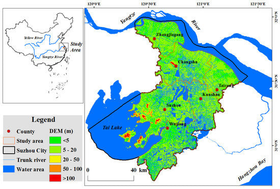
Figure 1.
Location of the study area. The trunk river shown in the figure is based on the data of the river systems in the 2010s. In order to represent a dense river system and a low and flat terrain as well, the digital elevation model (DEM) does not cover the trunk river and water area over the study area.
Suzhou City was selected as the study region because it (1) is a well-known region in China that is crisscrossed with water; (2) is currently one of the most developed regions in China; (3) has experienced in a short time two historic transformations, one to a traditional agriculture-based society and then one to a modern urbanized society. It should be noted that the study area did not contain waters of the Yangtze River and Tai Lake.
3. Materials and Methods
3.1. Land Use Data
Landsat 5 images (Thematic Mapper, TM) from 1983 and Landsat 8 images (Operational Land Imager, OLI) from 2014 were provided by Geospatial Data Cloud site, Computer Network Information Center, Chinese Academy of Sciences (http://www.gscloud.cn), which was systematically done using radiation calibration and geometric correction. Moreover, the spatial resolution of remote sensing images is 30 m, and the geographic coordinate system is the World Geodetic System 1984 and the projected coordinate system is the Universal Transverse Mercator.
Firstly, the remote sensing images were pretreated by layer stack, mosaic, mask, and so on; then, they were classified into the same four land use types: cultivated land, woodland, built-up land, and open water, by unsupervised classification in ERDAS IMAGINE software (version 9.2, Intergraph, Atlanta, GA, USA). Up to 200 test samples were randomly selected to assess the accuracy of the classification results in 1983 and 2014. Comparing the classification results with reference data (through visual interpretation), the results showed that the overall accuracy was 0.81 in 1983 and 0.80 in 2014, and the kappa coefficient was 0.64 in 1983 and 0.70 in 2014. Therefore, the quality of the classification results was very good and reliable.
3.2. River System Data
River system data were extracted from topographic maps at a 1:50,000 scale. Since compiling a topographic map needs several months or years at the early ages, the topographic maps of the study area spanned several years. Therefore, the river system data were named after chronology in this study. The river system data in the 1960s and 1980s were digitized from paper topographic maps compiled during 1964–1969 and 1978–1983, respectively. The river system data in the 2010s were derived from digitalized topographic maps compiled in 2014.
River systems are composed of planar rivers and linear rivers, according to the drawing specification of a topographic map. In practical terms, the area of the lake and reservoir was greater than 2500 m2. The planar river comprised a river and canal with a width greater than 20 m and is drawn on the map in a scale according to real spatial distribution and shape. For the linear river, the width of the river was between 10 m and 20 m and the width of the canal was less than 10 m; they are drawn as unified bold lines and fine lines, respectively [28,29].
As the flow direction of the rivers in Suzhou City is a rectilinear current affected by tide and the river network belongs to a trellis drainage pattern, the rivers cannot be graded by the Strahler method or the Shreve method. Because of the same difficulty in ordering rivers in Shanghai City, which abuts Suzhou City, the Shanghai Water Authority devised a river classification system that considers both natural features and the social roles of rivers, i.e., first-order (village level), second-order (town level), third-order (district level), and fourth-order (city level) rivers. This river classification system has been extended and applied in the Yangtze Delta, such as Suzhou, Wuxi, and Ningbo cities [22,30]. In this study, we borrowed this river classification system and defined a planar river as a first-order river (trunk river), bold line river as a second-order river (first tributary), and fine line river as a third-order river (second tributary), considering both the width and social attribute of the rivers (Table 1).

Table 1.
River systems were graded according to the width and social attribute.
3.3. Grid River Density
The grid river density (GRD) is a method to describe the quantitative characteristics of river systems in a grid. All operations of this method can be performed on ArcMap software (version 10.0, Environmental Systems Research Institute, Redlands, CA, USA) as follows:
- (1)
- Generating square boxes with side length ε through the Create Fishnet function, and each square box corresponding to a unique binary code.
- (2)
- Extracting the square boxes that intersect with the river systems through the Intersect function.
- (3)
- Calculating river density in each square box (i.e., the river density is equal to river length per area in a box scale) through the Field Calculator function.
- (4)
- Determining the optimal grid scale for calculating GRD. The approach is shown below:
There was a tendency that the mean GRD decreased with grid size (i.e., 1.0, 1.5, …,10.0 km), and the relationship between mean GRD and grid size was well fitted by the power function at each time (Figure 2), which indicates that the mean GRD has a scale effect [29,31]. The mean of the change-point method is a mathematical statistics method used to work out a turning point from steeply decreasing/increasing to gently decreasing/increasing of a fitted curve for nonlinear data, and the turning point is regarded as the optimal grid scale for calculating river density [32,33]. The mean of the change-point method can be described by the following equations:
where N is the sample number; is the sample mean; S is the square sum of deviations; i = 2,…,N; and Si is the difference between a sample’s two parts.
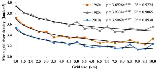
Figure 2.
Mean grid river density of the study area in different grid sizes. Grid size increased from 1.0 km to 10.0 km in 0.5 km increments. The relationship between mean grid river density (GRD) and grid size was well fitted by the power function at each time.
4. Results
4.1. Land Use Change
A transfer matrix of land use was constructed to quantitatively reflect the land use change from 1983 to 2014 (Table 2). Over time, land use was obviously different within the study area. The proportion of woodland and open water increased by 2.55% and decreased by 3.50% between 1983 and 2014. By contrast, land use change occurred mainly in cultivated land and built-up land. In 1983, the proportion of cultivated land was 62.05% while the proportion of built-up land was only 10.12%. Built-up land was concentrated in the older sections of Suzhou County (Figure 3). These indicated that cultivated land was the main land use type and agricultural production was a dominant part before 1983. As time went on, the proportion of cultivated land fell to 31.56% by 2014; the reduced cultivated land was converted mainly to built-up land. At the same time, the built-up land displaced cultivated land and turned to be the largest land use type; the proportion of built-up land increased to 41.55%. Such evidence indicates that Suzhou City experienced a transformation from an agrarian, rural economy to a highly urbanized economy from 1983 to 2014.
Table 2.
Transfer matrix of land use (%). Each cell in the matrix represents how land cover changed between two land use types between 1983 and 2014.
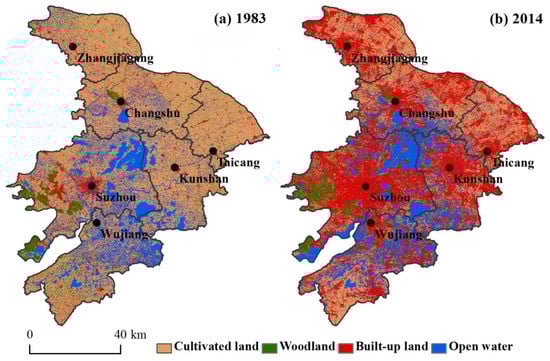
Figure 3.
Land use maps of the study area in 1983 (a) and 2014 (b) at a 30-m resolution.
4.2. River Systems Change
4.2.1. River Systems Change in Length
The length of the total rivers approximated 22,408 km by the 1960s but increased to 23,988 km by the 1980s and decreased to 21,379 km by the 2010s. Along with the time, the length of the first-order river firstly decreased slightly and then increased slightly while the length of the second-order river continued to fall substantially. However, the length of the third-order river firstly increased sharply and then decreased substantially (Figure 4). That is, agricultural modification (during the 1960s–1980s) was associated with a decrease in the length of the first-order river and second-order river but with an increase in the length of the third-order river; however, urbanization (during the 1980s–2010s) was associated with an increase in the length of the first-order river but with a decrease in the length of the second-order river and third-order river.
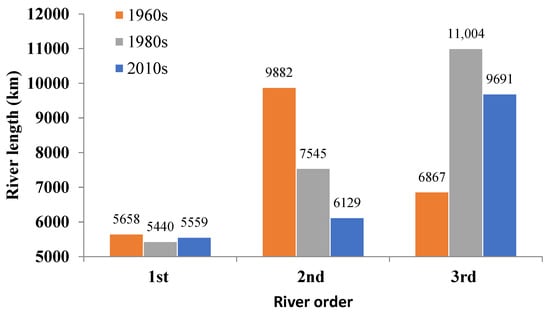
Figure 4.
River systems changed in length at each time.
4.2.2. Optimal Grid Scale
The existence of a turning point would make a growing gap between S and Si; therefore, the maximum difference value at a point was the turning point [29,32,33]. The difference value between S and Si firstly increased and then decreased and the maximum difference value was at point 6 for each time, i.e., the optimal grid scale for calculating GRD was 3 km × 3 km, as shown in Figure 5.
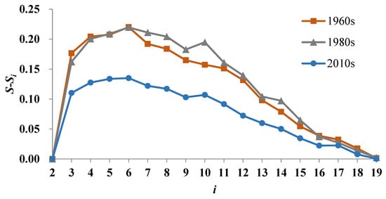
Figure 5.
Change curve of the difference value between S and Si at each time.
4.2.3. River Systems Change in GRD
The GRD was calculated on a 3 km × 3 km scale to reflect the spatial change of the river system, as shown in Figure 6. Different orders of rivers were remarkably different in the GRD changes during each period, as shown in Figure 6. For the first-order river, the decreased parts were slightly more than the increased parts during the 1960s–1980s with the opposite happening during 1980s–2010s; the increased parts focused on urban centers and neighboring areas (Figure 6a,b). The second-order river mostly decreased in GRD for each period, and the decreased parts during the 1960s–1980s were slightly more than during the 1980s–2010s (Figure 6c,d). For the third-order river, the GRD increase occurred in 71% of the region of the study area during the 1960s–1980s, while the GRD decrease occurred in 54% of the region of the study area during 1980s–2010s (Figure 6e,f). For total rivers, the GRD was mostly increased during the 1960s–1980s, and the increased parts accounted for 64% of the grids (Figure 6g). However, the GRD was almost opposite to the previous period during the 1980s–2010s; the increased parts accounted for only 38% of the grids while 61% of the grids decreased (Figure 6h).
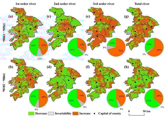
Figure 6.
River system changes in grid river density during the 1960s–1980s (a, c, e, g corresponding to first-order river, second-order river, third-order river and total river, respectively) and the 1980s–2010s (b, d, f, h corresponding to first-order river, second-order river, third-order river and total river, respectively). Each pie-chart in the lower right corner of the grid river density chart represents the percentage of grid river density that decreased, increased, or was unchanged.
For the variation in river length at a 3 km × 3 km scale, the length of the first-order river varied within a narrow range in both periods; the massive decrease in length of the second-order river and the massive increase in length of the third-order river were remarkable characteristics during the 1960s–1980s. The lengths of the second-order and third-order river were all decreased during the 1980s–2010s, and the decrease in length of the third-order river was more than that of the second-order river (Figure 7). Moreover, the lower the order of the river, the larger was the variation in the accumulated length (including increase and decrease). In addition, the accumulated length variation of the total rivers during the 1960s–1980s was greater than during the 1980s–2010s, which indicates that the river systems were more seriously transformed and disturbed during the agricultural modification period than during the urbanization period.
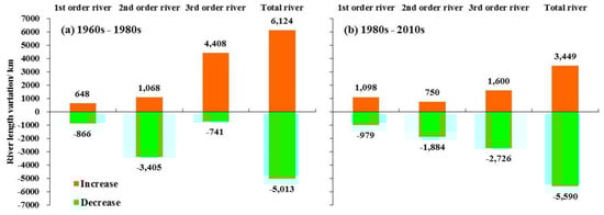
Figure 7.
River length changes during the 1960s–1980s (a) and the 1980s–2010s (b), using a 3 km × 3 km grid as the basic statistical unit. Note that (a, b) have the same vertical axis.
5. Discussion
5.1. Relationship between the Proportion of Cultivated Land and the Evolution of River Systems
In 1983, the proportion of built-up land was only 10.12% while the proportion of cultivated land was up to 62.05% (Table 2), which indicates that agriculture played a decisive role in the economic and social developments before 1983.
Figure 8 shows the relationship between the proportion of cultivated land and the corresponding mean GRD of the river system on a 3 km × 3 km scale in 1983. The mean GRD of the total rivers continued to increase until the proportion of cultivated land was 90%, and the increasing trend became slower as a whole. For different orders of rivers, the mean GRD firstly increased and then showed different change characteristics, i.e., the mean GRD of a first-order river and second-order river went down with a turning point at 70% and 80% cultivated land proportion, respectively, while the third-order river speeded up with a turning point at 80% cultivated land proportion. These results concur with those of Han et al. [21,34] who found that an increased river density was associated with agricultural water conservancy construction in the 1980s. Moreover, we speculate that undeveloped land was reclaimed to increase the amount of available arable land [25], but when the undeveloped land had been fully developed, the riverbanks were then reclaimed. In other words, when the proportion of cultivated land exceeded a threshold level, the higher order rivers were invaded, cut off, and even buried, which forced a part of the higher order rivers to transform into narrower rivers. However, in the agricultural areas of developed countries, rivers (including open ditches and channels) were replaced with subsurface drains [8] or were even buried [35] to provide more efficient access to the land. Therefore, the river system evolution varies from region to region under different agricultural modes.
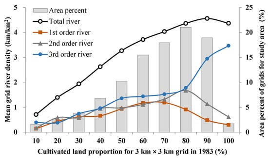
Figure 8.
Relationship between the proportion of cultivated land and the evolution of river systems. Note that the label “10” on the horizontal axis shows that the cultivated land proportion for a 3 km × 3 km grid is greater than or equal to 0 and less than 10, and so on.
5.2. Relationship between the Proportion of Built-Up Land and the Evolution of River Systems
The proportion of built-up land increased from 10.12% to 41.55% between 1983 and 2014, while the proportion of cultivated land decreased from 62.05% to 31.56% (Table 2). The land urbanization level (i.e., built-up land proportion) is an important indicator to estimate the level of urbanization [36]. Han et al. [21] used this indicator to estimate the urbanization level of counties in the Yangtze River Delta and defined counties with a land urbanization level under 30% as a low urbanization level and over 40% as a high urbanization level. Therefore, Suzhou City experienced a sharp urbanization process between 1983 and 2014.
Previous researchers showed that urbanization has a profound impact on river systems, and most researchers have concentrated on correlations between river indicators and impermeable surface coverage in watersheds or districts [20]. Figure 9 shows the relationship between the proportion of built-up land and the corresponding mean GRD of river systems on a 3 km × 3 km scale in 2014. The mean GRD of a first-order river and second-order river increased until the proportion of built-up land was 20%, and then smoothly fluctuated and tended to weakly decrease with an overall increase in the proportion of built-up land. However, the mean GRD of a third-order river first sharply increased and then continuously decreased; the corresponding turning point was a 40% proportion of built-up land. Similar results have been found in previous studies. The larger rivers (or higher order rivers) were usually dredged and reconstructed to meet the needs of flood protection and drainage during low urbanization levels in the Hangzhou-Jiaxing-Huzhou Plain [26] and the Tai Lake Watershed [28]. Moreover, in heavily urbanized portions of the Gunpowder-Patapsco Watershed, larger rivers were protected from burial by prominent riparian zones and environmental legislation [12]. In contrast, smaller rivers (or lower order rivers) were more extensively buried than larger rivers [3] and the difference increased with increasing impervious surface coverage in the Chesapeake Bay Watershed [35] and the Nansi Lake Basin [12]. In addition, some smaller rivers were widened and changed into larger rivers to improve the abilities of storage and discharge [28].
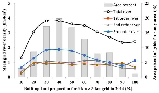
Figure 9.
Relationship between the proportion of built-up land and the evolution of river systems. Note that the label “10” in the horizontal axis shows that the built-up land proportion for a 3 km × 3 km grid is greater than or equal to 0 and less than 10, and so on.
It should be noted that with urbanization proceeding, there will more and more regions where the proportion of built-up land exceeds 40%, and more and more third-order river will be disturbed if we do not start to protect them now.
5.3. Analysis Accuracy and Uncertainty
River density is the most commonly used indicator for revealing the impact of land use change on river systems. In previous studies, watersheds [21], water conservation zones [22,23], and districts [24,25] were usually used as the basic unit for calculating river density. However, there are some limitations with these approaches, such as limited samples (from a few to hundreds of samples) and incompatible basic units (various areas for analysis units). Therefore, it is difficult to exactly depict the temporal and spatial characteristics of river systems. Accordingly, the analysis results about the relationship between land use change and river systems remain a great uncertainty. In this study, we presented a method of GRD that describes quantitative characteristics of river systems in an optimal grid scale. There are up to 826 samples in the study area and under the same analysis unit (3 km × 3 km grid). Moreover, it is easy to perform computation between GRD and raster data (e.g., land use data).
In this study, the phenomena and corresponding results only statically reflect the relationship between the proportion of cultivated land/built-up land and the evolution of river systems in 1983 and 2014 but is not enough to explain the impact of land use change on river systems during the agricultural modification/urbanization period. In addition, previous studies have demonstrated that the decision to change rivers can also be influenced by other regional landscapes, such as mean annual precipitation and soil type [35]. Therefore, further research should complete a comprehensive analysis (including natural and anthropogenic factors) to understand the mechanisms of river system evolution.
6. Conclusions
In this paper, river system evolution from the 1960s to 2010s in a river network plain was investigated, the temporal and spatial characteristics of river systems were analyzed through grid river density on a 3 km × 3 km scale, and the impacts of land use change on river systems in typical years were explored. The conclusions are as follows:
- (1)
- The length of the total rivers approximated 22,408 km by 1960s but increased to 23,988 km by 1980s and decreased to 21,379 km by 2010s. The grid river density of the total rivers was mostly increased during the 1960s–1980s but was almost opposite to the previous period during the 1980s–2010s. The spatial-temporal variation is very different for different order rivers.
- (2)
- The lower the order of the river, the larger was the variation in the accumulated length (including increase and decrease). River systems were transformed and disturbed more seriously during the agricultural modification period (1960s–1980s) than during the urbanization period (1980s–2010s), based on the variation in the accumulated length of the total rivers.
- (3)
- The river systems have been modified to meet the needs of human development in different social development stages. During the period of agricultural modification, undeveloped land was reclaimed to increase the amount of available arable land but when the proportion of cultivated land exceeded a threshold level, higher order rivers were invaded, cut off and even buried, which forced a part of higher order rivers to transform into narrower rivers. During the period of urbanization, higher order rivers were usually dredged, reconstructed and protected to improve the abilities of storage and discharge, and lower order rivers were buried after the proportion of built-up land exceeded 40%.
- (4)
- Compared with the traditional river density which concerns watersheds, water conservation zones, and districts as the basic unit, grid river density can quantify the spatial distribution of river systems on a finer spatial scale and can acquire more samples and higher analysis accuracy. Moreover, it is easy to perform a computation between grid river density and raster data (e.g., land use data).
Author Contributions
Y.X. and L.W. conceived the manuscript; L.W., J.Y., Y.X., and Q.W. collected and analyzed the data; L.W. wrote the paper, L.W., X.X. and H.W. proofread the paper.
Funding
This research was funded by the National Key Research and Development Program of China [2016YFC0401502], the National Natural Science Foundation of China [41771032, 41601018], the Water Conservancy Science and Technology Foundation of Jiangsu Province [2015003] and the State Foundation for Studying Abroad [201706190207].
Acknowledgments
The authors would like to express our thanks to the anonymous reviewers and the editors for useful ideas for improvement. Any errors and views expressed in this paper are the sole responsibility of the authors.
Conflicts of Interest
The authors declare no conflict of interest.
References
- Harden, C.P. Human impacts on headwater fluvial systems in the Northern and Central Andes. Geomorphology 2006, 79, 249–263. [Google Scholar] [CrossRef]
- Ollero, A. Channel changes and floodplain management in the meandering middle Ebro River. Geomorphology 2010, 117, 247–260. [Google Scholar] [CrossRef]
- Julian, J.P.; Wilgruber, N.A.; de Beurs, K.M.; Mayer, P.M.; Jawarneh, R.N. Long-term impacts of land cover changes on stream channel loss. Sci. Total Environ. 2015, 537, 399–410. [Google Scholar] [CrossRef] [PubMed]
- Strahler, A.N. The nature of induced erosion and aggradation. In Man’s Role in Changing the Face of the Earth; Thomas, W.L., Jr., Ed.; University of Chicago Press: Chicago, IL, USA, 1956. [Google Scholar]
- Wolman, M.G. A cycle of sedimentation and erosion in urban river channels. Geomorphology 1967, 49, 385–395. [Google Scholar]
- Chin, A. Urban transformation of river landscapes in a global context. Geomorphology 2006, 79, 460–487. [Google Scholar] [CrossRef]
- Napieralski, J.; Keeling, R.; Dziekan, M. Urban Stream Deserts as a Consequence of Excess Stream Burial in Urban Watersheds. Ann. Assoc. Am. Geogr. 2015, 105, 649–664. [Google Scholar] [CrossRef]
- Hietala-koivu, R.; Lankoski, J.; Tarmi, S. Loss of biodiversity and its social cost in an agricultural landscape. Agric. Ecosyst. Environ. 2004, 103, 75–83. [Google Scholar] [CrossRef]
- Steele, M.K.; Heffernan, J.B.; Bettez, N. Convergent Surface Water Distributions in U.S. Cities. Ecosystems 2014, 17, 685–697. [Google Scholar] [CrossRef]
- Napieralski, J.A.; Carvalhaes, T. Urban stream deserts: Mapping a legacy of urbanization in the United States. Appl. Geogr. 2016, 67, 129–139. [Google Scholar] [CrossRef]
- Kaushal, S.S.; Belt, K.T. The urban watershed continuum: Evolving spatial and temporal dimensions. Urban Ecosyst. 2012, 15, 409–435. [Google Scholar] [CrossRef]
- Elmore, A.J.; Kaushal, S.S. Disappearing headwaters: Patterns of stream burial due to urbanization. Front. Ecol. Environ. 2008, 6, 308–312. [Google Scholar] [CrossRef]
- Wheeler, A.P.; Angermeier, P.L.; Rosenberger, A.E. Impacts of New Highways and Subsequent Landscape Urbanization on Stream Habitat and Biota. Rev. Fish. Sci. 2005, 13, 141–164. [Google Scholar] [CrossRef]
- Nilsson, C.; Reidy, C.A.; Dynesius, M.; Revenga, C. Fragmentation and flow regulation of the world’s large stream system. Science 2005, 308, 405–408. [Google Scholar] [CrossRef] [PubMed]
- Yin, Y.X.; Xu, Y.P.; Chen, Y. Relationship between Changes of River-lake Networks and Water Levels in Typical Regions of Taihu Lake Basin, China. Chin. Geogr. Sci. 2012, 22, 673–682. [Google Scholar] [CrossRef]
- Sear, D.A.; Newson, M.D. Environmental change in river channels: A neglected element. Towards geomorphological typologies, standards and monitoring. Sci. Total Environ. 2003, 310, 17–23. [Google Scholar] [CrossRef]
- Vanacker, V.; Molina, A.; Govers, G.; Poesen, J.; Dercon, G.; Deckers, S. River channel response to short-term human-induced change in landscape connectivity in Andean ecosystems. Geomorphology 2005, 72, 340–353. [Google Scholar] [CrossRef]
- Gregory, K.J.; Davis, R.J.; Downs, P.W. Identification of river channel change due to urbanization. Appl. Geogr. 1992, 12, 299–318. [Google Scholar] [CrossRef]
- Burt, T.P. Monitoring change in hydrological systems. Sci. Total Environ. 2003, 310, 9–16. [Google Scholar] [CrossRef]
- Walsh, C.J.; Roy, A.H.; Feminella, J.W.; Cottingham, P.D.; Groffman, P.M.; MorGan, R.P. The urban stream syndrome: Current knowledge and the search for a cure. J. N. Am. Benthol. Soc. 2005, 24, 706–723. [Google Scholar] [CrossRef]
- Han, L.F.; Xu, Y.P.; Lei, C.C.; Liu, Y.; Deng, X.J.; Hu, C.S.; Xu, G.L. Degrading river network due to urbanization in Yangtze River Delta. J. Geogr. Sci. 2016, 26, 694–706. [Google Scholar] [CrossRef]
- Yang, K.; Yuan, W.; Zhao, J.; Xu, S.Y. Stream structure characteristics and its urbanization responses to tidal river system. Acta Geogr. Sin. 2004, 59, 557–564. [Google Scholar]
- Yuan, W.; Yang, K.; Wu, J.P. River structure characteristics and classification system in river network plain during the course of urbanization. Sci. Geogr. Sin. 2007, 27, 401–407. [Google Scholar]
- Xu, H.; Yang, S.J. Exploring the evolution of river networks in plain polders of Taihu Lake basin. Adv. Water Sci. 2013, 24, 366–371. [Google Scholar]
- Deng, X.J.; Xu, Y.P.; Han, L.F.; Li, G.; Wang, Y.F.; Xiang, J.; Xu, G.L. Spatial-temporal changes of river systems in Jiaxing under the background of urbanization. Acta Geogr. Sin. 2016, 71, 75–85. [Google Scholar]
- Xu, G.L.; Xu, Y.P.; Wang, L.Y. Temporal and spatial changes of river systems in Hangzhou-Jiaxing-Huzhou Plain during 1960s–2000s. Acta Geogr. Sin. 2013, 68, 966–974. [Google Scholar]
- Huang, Y.L.; Wang, Y.L.; Liu, Z.H. Stream construction characteristics in rapid urbanization area: Shenzhen city as a case. Geogr. Res. 2008, 27, 1212–1220. [Google Scholar]
- Deng, X.J.; Xu, Y.P.; Han, L.F.; Song, S.; Liu, Y.; Li, G.; Wang, Y.F. Impacts of Urbanization on River Systems in the Taihu Region, China. Water 2015, 7, 1340–1358. [Google Scholar] [CrossRef]
- Wu, L.; Xu, Y.P.; Xu, Y.; Yuan, J.; Xiang, J.; Xu, X.; Xu, Y. Impact of rapid urbanization on river system in river network plain. Acta Geogr. Sin. 2018, 73, 104–114. [Google Scholar]
- Zhao, J.; Lin, L.Q.; Yang, K.; Liu, Q.X.; Qian, G.G. Influences of land use on water quality in a reticular river network area: A case study in Shanghai, China. Landsc. Urban Plan. 2015, 137, 20–29. [Google Scholar] [CrossRef]
- Yu, G.M.; Wu, L.; Yu, Q.W. Scale dependence of landscape indices based on the analysis of land use database. Open Trans. Geosci. 2014, 2, 34–49. [Google Scholar] [CrossRef]
- Chen, X.X.; Chang, Q.R.; Guo, B.Y.; Zhang, X.J. Analytical study of the relief amplitude in China based on SRTM DEM data. J. Basic Sci. Eng. 2013, 21, 670–678. [Google Scholar]
- Chang, Z.Y.; Wang, J.; Bai, S.B.; Zhang, Z.G. Determination of accumulation area based on the method of applying mean of change-point analysis. J. Nanjing Norm. Univ. 2014, 1, 147–150. [Google Scholar]
- Han, L.F.; Xu, Y.P.; Yang, L.; Deng, X.J.; Hu, C.S.; Xu, G.L. Temporal and spatial change of stream structure in Yangtze River Delta and its driving forces during 1960s–2010s. Acta Geogr. Sin. 2015, 70, 819–827. [Google Scholar]
- Stammler, K.L.; Yates, A.G.; Bailey, R.C. Buried streams: Uncovering a potential threat to aquatic ecosystems. Landsc. Urban Plan. 2013, 114, 37–41. [Google Scholar] [CrossRef]
- Wang, Y.; Wang, S.J.; Qin, J. Spatial evaluation of land urbanization level and process in Chinese cities. Geagr. Res. 2014, 33, 2228–2238. [Google Scholar]
© 2018 by the authors. Licensee MDPI, Basel, Switzerland. This article is an open access article distributed under the terms and conditions of the Creative Commons Attribution (CC BY) license (http://creativecommons.org/licenses/by/4.0/).