Hydrological Process Simulation of Inland River Watershed: A Case Study of the Heihe River Basin with Multiple Hydrological Models

Abstract

Simulating the hydrological processes of an inland river basin can help provide the scientific guidance to the policies of water allocation among different subbasins and water resource management groups within the subbasins. However, it is difficult to simulate the hydrological processes of an inland river basin with hydrological models due to the non-consistent hydrological characteristics of the entire basin. This study presents a solution to this problem with a case study about the hydrological process simulation in an inland river basin in China, Heihe River basin. It is divided into the upper, middle, and lower reaches based on the distinctive hydrological characteristics in the Heihe River basin, and three hydrological models are selected, applied, and tested to simulate the hydrological cycling processes for each reach. The upper reach is the contributing area with the complex runoff generation processes, therefore, the hydrological informatic modeling system (HIMS) is utilized due to its combined runoff generation mechanisms. The middle reach has strong impacts of intensive human activities on the interactions of surface and subsurface flows, so a conceptual water balance model is applied to simulate the water balance process. For the lower reach, as the dissipative area with groundwater dominating the hydrological process, a groundwater modeling system with the embedment of MODFLOW model is applied to simulate the groundwater dynamics. Statistical parameters and water balance analysis prove that the three models have excellent performances in simulating the hydrological process of the three reaches. Therefore, it is an effective way to simulate the hydrological process of inland river basin with multiple hydrological models according to the characteristics of each subbasin.

1. Introduction

Hydrological models are important tools for simulating hydrological cycling processes for water resource assessment, management, and utilization [1]. Since the concept of unit hydrograph was produced by Sherman [2], the development of hydrological models experienced three stages. The first one is about the knowledge exploration of the infiltration, evaporation, and streamflow concentration, which are the critical parts of hydrological cycling processes. Based on the accumulation of hydrological knowledge, lumped hydrological models are developed including Stanford model [3], Soil Conservation Service model (SCS) [4], Xinanjing Model [5]. After the concept of distributed hydrological model was introduced by Freeze and Harlan [6], distributed models are developed and widely applied, such as Soil and Water Assessment Tool (SWAT) [7], Hydrologic System Program Fortran (HSPF) [8], and Variable Infiltration Capacity model (VIC) [9].

Hydrological model development considers the spatial heterogeneity with the model structure and description of hydrological processes [10]. The study area has been discretized into sub-watersheds [11], grid cells [9], representative elementary areas (REA) [12], and hydrological response units (HRU) [7] based on digital elevation models (DEMs), land cover, and soil datasets with the technologies of geographical information system and remote sensing. Hydrological models define them as the basic spatial simulating unit, on which the hydrological cycling process is simulated. The spatial heterogeneity of hydrological model input about precipitation is presented with the monitoring meteorological stations together with the interpolation methods of Kriging, ridge regression, and inverse distance weighted (IDW) [13].

Spatial heterogeneity is considered when representing hydrological processes by hydrological models about the runoff generation and streamflow channel routing. Xinanjiang model presents the soil infiltration with the probability distribution function based on the variable infiltration capacity accounting for the soil properties [5]. Soil Conservation Service developed the curve number method to determine the rainfall–runoff relationship and coefficients based on the soil, land cover, and slope [4]. The runoff generation mechanisms of saturation excess dominated in the humid area and intensity excess in the arid area are combined with time compression analysis method [9,14] to increase the runoff predicting accuracy in semi-arid areas. Regarding channel routing, the kinematic wave model described the overland flow concentration process accounts for the distance of hillslope, surface roughness, and slope. The lumped overland flow concentration method GIUH adds the geomorphological characteristics into the instantaneous unit hydrograph [15,16] in estimating the streamflow concentration time, velocity, and quantity. Distributed channel routing models, such as Saint-Venant equations, estimate the flow rate, velocity, and depth along the channels considering distance along watercourse, cross section area, and the watercourse bottom slope with the numerical solutions working under different basin hydrological conditions [17].

Even though spatial heterogeneity has been considered in hydrological model development, no single hydrological model can be applied under all conditions. Therefore, exclusive models are developed in describing the hydrological processes with distinctive characteristics and applied in appropriate areas. For urban areas with subsurface pipe-nets, storm water management model (SWMM) [18] is applied to simulate the runoff quantity and quality by describing the streamflow concentration and subsurface water movement through pipe-nets. In the ground water dominated watersheds, groundwater model MODFLOW model is developed and applied to estimate the groundwater quantity through describing the water balance processes and physical mechanism of the groundwater dynamics [19,20]. In glacierized watersheds, the streamflow is estimated through describing the processes of melt water from glaciers draining to the catchment outlet with the coupled model HBV and the glacier retreat model developed by Li et al. [21].

The characteristics of an inland river basin in regards to the hydrological cycling process are not consistent over the entire basin, with the upper subbasin as the contributing area, and middle and lower subbasins as the dissipative areas. It is hard to obtain excellent simulating results utilizing one hydrological model, much less to provide scientific support about the water allocation among different subbasins and water resource management within the subbasins, even though spatial heterogeneity is considered in hydrological models such as VIC, SWAT, or exclusive models. Therefore, this study presents a solution to simulate the hydrological process of an inland river basin with multiple hydrological models by providing a case study of the hydrological process simulation of the Heihe River basin in China. Three hydrological models are selected, applied, and tested in simulating the hydrological processes of the upper, middle, and lower reaches of Heihe River basin respectively, according to the distinctive hydrological characteristics of the three subbasins of Heihe River basin.

2. Materials and Methods

2.1. Study Area

Heihe River basin is the second largest inland river basin in China with a drainage area of 14.29 × 10⁴ km² located in the northwestern China (98°34′–101°09′ E, 39°09′–37°43′ N). Heihe River goes over three provinces, Qinghai, Gansu, and Inner Mongolia, and then disappears in Inner Mongolia due to evaporation and baseflow recharge. The Heihe River basin goes through semi-arid, arid, and extremely arid areas, therefore, it has been divided into three subbasins with two valleys: Yingluoxia valley and Zhengyixia valley (Figure 1). The study area is the three reaches of the mainstream located in the three subbasins.

The upper reach is the contributing area of the entire Heihe River basin, gauged at Yingluoxia hydrological station with the drainage area of 10,000 km², and elevation of 1673–5011 m (Figure 1 and

Table 1. Parameters of the three reaches.

Parameters	Heihe River	Upper Reach	Middle Reach	Oasis Area (Lower Reach)
Area (104 km2)	11.6	1	2.56	3.4
ET (mm)	800–2200	800–1200	1200–1800	>2000
Air temperature (°C)	2.0–8.0	2.0–1.5	2.8–7.6	8.0
Streamflow (mm)	30	100–200	50–100	50–5
P (mm)	30–420	300–600	100–300	30–100
Arid index		<3.0	3.0–10.0	>10.0
River length (km)	821	303	185	333
Elevation		3000–3500	1000–2600	1000–1500

Note: Arid index = ET_a/P.

). It provides nearly 70% of the streamflow in the entire study domain, which supplies agricultural irrigation and benefits the social economy development in the middle and lower basins [22]. This reach belongs to the semi-arid area with annual precipitation of 360 mm, annual average air temperature of −3 to 1 °C, and evaporation of 800–1200 mm. The precipitation of June to September accounts for 73% of the annual precipitation quantity. The streamflow is recharged by precipitation in summer and snowmelt in spring. The dominant soil types are Alpine meadow soil, chestnut soil, alpine frost soil, and calcareous soil. Land is covered by grass (51%), forests (21%), and unused areas (24%).

The middle reach is the dissipative area of the entire Heihe River basin, and gauged at Zhengyixia hydrological station with the drainage area of 2.56 × 10⁴ km² and elevation of 1000–2600 m (Figure 1 and Table 1). It is in the arid Gobi Desert with the annual average air temperature of 2.7 to 8 °C, arid index of 3.0–10.0, annual precipitation from 100 to 300 mm, and annual ET from 1200 to 1800 mm. This area is covered with 29.2% grassland and 41.4% unused area, and other land covers include agricultural area (16%), forest land (9.7%), and bare soil (3.7%). As more than 90% residents of the Heihe River basin concentrate in the middle reach, interactions between the surface streamflow and subsurface flow are prompted by the intensive human activities [23] such as constructing water supply projects, developing irrigated agriculture, reclaiming fallow land, etc.

The lower reach is the other dissipative area of the Heihe River basin, and an oasis is located in the lower subbasin of the Heihe River Basin (Figure 1) with an area of 3.4 × 10⁴ km² and mean elevation around 1000 m. It belongs to the extremely arid area with annual precipitation less than 100 mm, average annual air temperature 8.2 °C, potential evapotranspiration more than 2000 mm, and arid index greater than 10.0. The land cover is sparse vegetation dominated by xeric shrubs and subshrubs. Due to the extremely arid climate, the streamflow of Heihe River eventually disappears in this area through evaporation and baseflow recharge, and the groundwater is the dominant water resource for the maintenance of the oasis ecosystem. Figure 2 indicates the geo-tectonic structure of the oasis. The underground aquifer system is composed of unconsolidated Quaternary sediments of 100–200 m [24,25]. The aquifers vary from a zone to a multilayered zone [24,26] with the lithological features varied gradually from gravel and pebbles to fine sands and silts [25].

2.2. Streamflow Simulating Systems of the Heihe River Basin

According to the hydrological characteristics of the three reaches, three different hydrological models are selected and applied to simulate the hydrological processes of the three reaches correspondingly. The HIMS model is utilized for the upper reach due to the semi-arid climate with runoffs generated by both the mechanisms of intensity excess and saturation excess [1]. The water balance model is developed for the middle reach based on the frequent interactions of surface and subsurface flows prompted by the human activities. The groundwater modeling system (GMS7.0) [27] imbedded with MODFLOW is applied in the lower reach to simulate the water cycling process dominated by the groundwater dynamics (

Table 2. The model simulating systems for each reach.

Reach	Model	Source
Upper reach	HIMS	Wang et al. [1]
Middle reach	Water balance model	Li, 2005 [28]
Lower reach	GMS	Owen et al. [27]

).

2.2.1. HIMS Model of the Upper Reach

HIMS model is selected to simulate the hydrological process of the upper reach, as it has the structure of combined runoff generation mechanisms of intensity excess and saturation excess, and the snow module composed with equations of degree-day and energy conservation. Details of HIMS model can be found in Wang et al. [1], while it is briefly introduced here for clarity. This model has the grid cell or sub-watershed as its basic unit of water cycling process, as indicated by Figure 3. In each grid cell/sub-basin, nine processes of hydrological cycling, namely, precipitation, Evapotranspiration (ET), snowmelt, interception, infiltration, surface flow, subsurface flow, and baseflow, are described. Precipitation falls on the ground as rainfall or snow after interception process, and the actual ET is simulated for each vegetation type accounting for the impacts of LAI and soil moisture of root zone. Soil of each grid cell or sub-basin is divided into three layers: root zone, transition zone, and the saturated layer for integration with the crop model which describes the crop biomass accumulation processes and communicates with hydrological model with actual ET and irrigation (Figure 3). Surface flow, lateral flow, and the partial baseflow of three soil layers are combined as streamflow leaving the hillslopes and heading for the reservoirs/lakes or changing into ET. The rest of the baseflow from hillslopes goes into the next sub-watershed through ground water directly, as a way to describe the sub-watersheds water communication through underground water movement. In the simulating frame of HIMS for the upper reach, ET is estimated with the Hargreaves equation [29]; snowmelt is calculated with the Degree-Day equation and energy balance equation; the runoff generation modular is LCM [30], and the channel routing routine is the Muskingum model [31] which clarifies the streamflow concentrating process. The upper reach has been divided into 152 grid cells with resolution of 10 km × 10 km. The observed dataset of streamflow from Yingluoxia hydrological station is used for the model calibration and validation.

2.2.2. Water Balance Model of the Middle Reach

Due to the intensive interactions of surface and subsurface flows under the impacts of human activities in the middle reach, a conceptualized water balance model is developed and applied to simulate the hydrological process. This model is based on the water conservation principle accounting for the inflow and outflow items of the entire middle reach with the involvement of the water balance equations of the six major land covers and water communications among the six land covers. The water balance equations are developed for each land cover and listed in

Table 3. Equations of the concept water balance model for the middle reach.

Number	Area	Water Balance Equations
1	Entire middle reach	$Pre+R_{in}+D=E+R_{out}$
2	Agricultural land	$\Delta S_1=P_1+U_{in1}+G_1-E_1-R_1-I_1$
3	Forest land	$\Delta S_2=P_2+U_{in2}-E_2-R_2-I_2$
4	Grass land	$\Delta S_3=P_3+U_{in3}-E_3-R_3-I_3$
5	Urban area	$\Delta S_5=P_5+U_{in5}-E_5-R_5$
6	Water area	$\Delta S_4=P_4+R_{in}+M_4+Q_4-R_{out}-U_{out4}-E_4-I_4$
7	Unused area	$\Delta S_6=P_6-R_6-E_6-I_6$
	Parameter	Equations
8	Water storage change	$\Delta S_7=D-G_1-Q_4+I_1+I_2+I_3+I_4+I_5+I_6$
9	Infiltration	$I=k\left(P+U_{in}\right)$
10	Surface flow	$R=\alpha *P$
11	Actual ET	$E{T}_c=K_s*K_c*E{T}_0=\beta *E{T}_0$

Note: P_re is the precipitation quantity, R_in is the inflow of Yingluoxia station, D is the lateral recharge quantity, E is the evaporation quantity, Rout is the outflow of Zhengyixia station; ∆S is the water storage change, U_in is the surface inflow, G is the subsurface inflow, R is the quantity of generated runoff, I is the infiltrated water quantity (subscript: 1, agricultural land; 2, forestland; 3, grassland; 4, water area; 5, urban area; 6, unused land; 7, entire middle reach), M₄ is the inflow concentrated into the water area, Q₄ is the spring outflow, k is the percolation coefficient, N is the surface flow quantity, α is the runoff generation coefficient, ET_c is the ET of water saving crops, ET₀ is the ET of referencing crops, K_c is the crop coefficient, K_s is the adjustment coefficient of soil moisture, and β is the ET coefficient obtained through timing K_c with K_s.

according to the characteristics of water cycling process of each land cover type. Flow communications among the six land covers are realized through infiltration, groundwater extraction, and spring outlet with Equations (1) and (8) in Table 3. The basic structure of the water balance model is shown in Figure 4 for the entire middle reach. The study area has been divided into 262 grid cells with resolution of 10 km × 10 km, based on which the model is run. Model inputs for the entire middle reach are the precipitation, the maximum and minimum air temperatures, surface water inflow, subsurface water inflow, recharge of lateral flow, and streamflow from the upper reach. The model outputs are ET and the streamflow of the middle reach.

2.2.3. MODFLOW Application to the Lower Reach

The hydrological process of the lower reach is dominated by the groundwater dynamics due to the extreme arid climate. The hydrological cycling process of the lower reach is simulated with the ground water system (GWS) which is a software program for groundwater simulation with a collection of the preeminent groundwater models [27]. The modules of GWS applied in this study are shown in Figure 5. The streamflow evaporation and infiltration vertically, and outflow horizontally of each grid cell are simulated with streamflow-routing 2 (SFR2) model. The groundwater movement from aquifers is simulated with MODFLOW [32]. The MODFLOW is a finite-difference groundwater model, which has the aquifer divided into different layers in the vertical direction and into grid cells at the horizontal level for each layer. Inputs of MODFLOW are river stage, groundwater recharge, water transfer, drainage, aquifer ET. Outputs are the cell based recharge, aquifer-river exchange rate, variation of GW head, drainage, and aquifer ET.

The lower reach has been horizontally divided into 43,891 cells of 500 m × 500 m, and three layers of the aquifer vertically: phreatic aquifer, aquiclude, and the confined aquifer. Six zones are identified (Figure 1) within which aquifer parameters are the same, according to groundwater dynamics analysis [25]. The geological difference among the three layers and six parameter zones are presented with three hydrogeological parameters of the aquifer: the horizontal and vertical infiltration rates of water storage (K and K_z, respectively) and the rate of water storage (μ). Water recharges of the oasis are streamflow from the middle reach, the precipitation, and the infiltration of the surface flow and irrigation. Outputs of the oasis are the ET and groundwater extraction. Hydrological simulation is focused on the vertical flow interaction and the baseflow movement.

2.3. Observed Datasets

For the three reaches of the Heihe River basin, DEM and land cover maps from 2005 with a resolution of 30 m × 30 m are obtained from the Data Center of Environmental and Ecological sciences of Western China (http://westdc.westgis.ac.cn). Soil dataset with a resolution of 1 km × 1 km is from the Data Center of Environmental Sciences of Chinese Academy. The climate dataset of the upper reach is obtained through interpolation with the Thiessen polygons method based on the datasets of four meteorological stations shown in Figure 1: Tuole station, Yeniugou station, Minle station, and Sunan Station. It includes precipitation and maximum air temperatures from 1960 to 2010 at daily time step. The observed streamflow dataset of the upper reach comes from Yingluoxia station from 1976 to 1998 with the absence from 1987 to 1990 at daily time step. It is used for HIMS model calibration from 1979 to 1987 and validation from 1990 to 1998.

For the middle reach, climate dataset is obtained through interpolation with the Thiessen polygons method based on the observed datasets from eight meteorological stations shown in Figure 1: Shandan station, Zhangye station, Jiuquan station, Tuole station, Yeniugou station, Qilian station, Alashanyouqi station, and Yongchang station. It includes precipitation and air temperature from 1960 to 2009 at monthly time step. The dataset of monthly surface water division quantity, groundwater division quantity, and the observed lateral flow recharge from the upstream basin is obtained from Yearbook of Heihe River from 2000 to 2009. The observed streamflow dataset of Zhengyixia station is from 1977 to 2009 at monthly time step, and used for model calibration from 1980 to 1989 and model validation from 1990 to 2009.

For the lower reach, the climate dataset comes from Ejina meteorological station from 2000 to 2009 at daily time step, and includes the precipitation, air temperature, and the maximum evaporation. Observed streamflow of the same period comes from Langxinshan hydrological station at daily time step and is processed into monthly time step as the model input. Groundwater levels of the 15 wells located in the oasis area shown in Figure 1 are recorded once per 10 days from 2000 to 2008 and once per 30 min from 2009 to 2011. The observed datasets of groundwater level depth of 15 wells are used for the model calibration and validation from 2000 to 2005 and from 2006 to 2011, respectively.

Statistical parameters used to evaluate the model performance in estimating streamflow are Nash–Sutcliffe efficiency (NSE), water error (WE), and the root mean square error observations standard deviation ratio (RSR). NSE describes the fitting extent between simulation and observation datasets on streamflow. WE evaluates the predicting accuracy of HIMS about streamflow quantity. RSR is recommended by Moriasi et al. [33] for testing the streamflow simulation. If NSE is greater than 0.5, the RSR is less than 0.6, and the WE is within the range of ±10%, then the simulating results are regarded to be satisfactory. The mean absolute error (MAE) and the root mean square (RMS) are used to evaluate the GMS performance in groundwater level simulation and are statistically satisfied with values less than or equal to 0.5.

$$\mathrm{NSE}=1-\frac{{{\displaystyle \sum }}_{\mathrm{i}=1}^{\mathrm{n}}{({\mathrm{Y}}_{\mathrm{i}}^{\mathrm{obs}}-{\mathrm{Y}}_{\mathrm{i}}^{\mathrm{sim}})}^2}{{{\displaystyle \sum }}_{\mathrm{i}=1}^{\mathrm{n}}{({\mathrm{Y}}_{\mathrm{i}}^{\mathrm{obs}}-{\mathrm{Y}}^{\mathrm{mean}})}^2}$$

(1)

$$\mathrm{WE}=\frac{{{\displaystyle \sum }}_{\mathrm{i}=1}^{\mathrm{n}}{\mathrm{Y}}_{\mathrm{i}}^{\mathrm{obs}}-{{\displaystyle \sum }}_{\mathrm{i}=1}^{\mathrm{n}}{\mathrm{Y}}_{\mathrm{i}}^{\mathrm{sim}}}{{{\displaystyle \sum }}_{\mathrm{i}=1}^{\mathrm{n}}{\mathrm{Y}}_{\mathrm{i}}^{\mathrm{obs}}}\times 100\%$$

(2)

$$\mathrm{RSR}=\frac{\sqrt{{{\displaystyle \sum }}_{\mathrm{i}=1}^{\mathrm{n}}{({\mathrm{Y}}_{\mathrm{i}}^{\mathrm{obs}}-{\mathrm{Y}}_{\mathrm{i}}^{\mathrm{sim}})}^2}}{\sqrt{{{\displaystyle \sum }}_{\mathrm{i}=1}^{\mathrm{n}}{({\mathrm{Y}}_{\mathrm{i}}^{\mathrm{obs}}-{\mathrm{Y}}^{\mathrm{mean}})}^2}}$$

(3)

$$\mathrm{MAE}=\frac{1}{\mathrm{n}}{\displaystyle \sum }_{\mathrm{i}=1}^{\mathrm{nw}}{\left({\mathrm{h}}_{\mathrm{m}}-{\mathrm{h}}_{\mathrm{s}}\right)}_{\mathrm{i}}$$

(4)

$$\mathrm{RMS}=\sqrt{\frac{{{\displaystyle \sum }}_{\mathrm{i}=1}^{\mathrm{nw}}{\left({\mathrm{h}}_{\mathrm{m}}-{\mathrm{h}}_{\mathrm{s}}\right)}^2}{\mathrm{nw}}}$$

(5)

where Y_i^obs is the ith observation; Y_i^sim is the ith simulated value; Y^mean is the mean of observed data; n is the number of dataset; h_m and h_s are the observed and simulated values of aquifer’s hydraulic head, respectively; and nw is the total number of the monitoring wells.

3. Results and Discussion

3.1. Streamflow Simulation of the Upper Reach

The simulated streamflow of the upper reach with HIMS model is compared with the observed streamflow in Figure 6 at monthly time step and the statistical evaluating results are listed in

Table 4. The statistical results of streamflow simulations of the upper and middle reaches.

Monthly	Calibration			Validation
	NSE	WE (%)	RSR	NSE	WE (%)	RSR
Upper reach	0.97	6.1	0.44	0.97	6.9	0.44
Middle reach	0.72	9.4	0.46	0.68	−9.74	0.53

. The simulated streamflow well fits the observation in both the calibration and validation periods with the exception of the streamflow peaks generated by the extreme storm events. To ensure the streamflow simulation performance of HIMS model with one set of parameters for the many precipitation events, less attention is paid to the extreme storm events in the calibration process. The statistical results for the comparison of simulated and observed streamflow are satisfied at monthly time steps. HIMS model has better performance in streamflow estimation than the SWAT model with NSE 0.93 obtained by Yang et al. [34] and VIC model with NSE 0.62 by He et al. [35] for the same study area and time periods at monthly time step. It is probably due to the combined runoff generation mechanism structure of HIMS model about intensity excess and saturation excess.

The simulated streamflow indicates the characteristics of the semi-arid upper reach. It is low in winter (November to March) as the streamflow mainly comes from the groundwater, increases in spring (April to June) due to the snowmelt caused by the air temperature, and increases quickly in summer (July to September) as a result of the frequent precipitation events. Small streamflow peaks are created in May/June by the snowmelt water, while the streamflow peak in July to September are produced by rainfall. The water balance is closed in both the calibration and validation periods with the involvement of precipitation including rainfall and snow, actual ET, streamflow with snow water equivalent (SWE) and runoff, and the change of soil moisture at annual time step (

Table 5. Water balance status of the upper reach of Heihe River Basin.

Upper Reach	Precipitation (mm/year)		A.E.T.* (mm/year)	Streamflow (mm/year)		$\mathbf{\Delta }$ Soil Moisture (mm/year)
	Rain	Snow		Runoff	SWE*
Calibration period	331.4	25.7	196.6	148.9	7.8	3.8
Validation period	329.9	30.7	204.3	148	9.4	−1.1

Note: SWE* denotes snow water equivalent. A.E.T.* denotes the actual evapotranspiration.

). In the upper reach, the major inflow is rain of 330 mm and snow of 25.7–30.7 mm. The two major outflows are the actual ET and streamflow with ET being greater than the streamflow. The streamflow obtains runoff of 156 mm generated by precipitation and SWE of 7.8–9.4 mm produced by snow. Therefore, the snowmelt is a streamflow source but not the major one relative to the rainfall for the upper reach as the contributing area for the entire Heihe River basin.

3.2. Water Balance Analysis of the Middle Reach

The water balance model is applied to estimate the streamflow and simulate the hydrological process of the middle reach. Streamflow comparison between the simulation and observation is shown in Figure 7 at monthly time step in the calibration and validation periods. The model performs well in estimating the streamflow indicated by the evaluating statistical result with NSE exceeding 0.65, WE within ±10%, and RSR less than 0.6 (Table 4). The error mainly comes from July to September on agricultural land, due to the alternation of the three months’ inflows from 2001 to 2006 with the average monthly inflows from 2007 to 2009 as a result of missing data for the surface streamflow and groundwater division during the three months for the agricultural land.

The middle reach is the dissipative area with six major land covers, water balance is closed for each land cover based on the annual averaged inflows and outflows from 2001 to 2009 (

Table 6. Inflows of the six land use types of the middle reach of Heihe River.

Land Uses	Area (%)	P* (mm)	Uin* (mm)	Gin* (mm)	Rin* (mm)	Surface Flow (mm)	Spring Outflow (mm)
Water area	2.3	161.82	-	-	2760.90	985.44	1362.12
Agricultural Land	16.1	156.49	409.76	99.14	-	-	-
Forestland	9.7	280.20	47.16	-	-	-	-
Grassland	29.2	207.39	6.48	-	-	-	-
Urban area	1.3	99.82	158.54	-	-	-	-
Unused area	41.3	146.49	-	-	-	-	-

Note: P* is the precipitation; U_in* is the surface flow division; G_in* is the groundwater division; R_in* is the input of streamflow from the upstream basin.

and

Table 7. Outflows of the six land use types of the middle reach of Heihe River basin.

Land Uses	E.T. (mm)	Streamflow (mm)	Percolation (mm)	Drainage (mm)	Outflow (mm)	Uout (mm)
Water area	219.62	-	399.60	-	1415.13	3236.46
Agricultural Land	461.69	31.30	172.31	-	-	-
Forestland	241.30	50.44	35.76	-	-	-
Urban area	69.24	45.51	-	142.69	-	-
Grassland	174.96	33.18	5.71	-	-	-
Unused area	144.57	1.46	0.46	-	-	-

Note: U_out is water division.

). The streamflow is mainly recharged by the precipitation and inflow from the upper reach for the water areas, while precipitation and the surface flow division are the two sources for the other areas with five land covers. Agricultural land plays the dominant role in influencing the water balance status of the entire middle reach, as it has the greatest inflow and water consumption of 665.39 mm and 665.31 mm among all land use types except water area. Although the inflow is the artificial water division and precipitation, artificial water division is the major inflow for the agricultural land, as it is greater than the precipitation. ET is the primary outflow item for the agricultural land followed by percolation (Table 7). The water consumptions of forest and grasslands are both lower than agricultural land with the precipitation and ET as the major inflow and outflow items (Table 6 and Table 7). This finding supports the conclusion of Sang et al. [36] that the increased air temperature decreases runoff quantity through increasing ET in the middle reaches, although it increases runoff in the upper reach in spring by the accelerating the snowmelt process.

For the entire middle reach, water balance is kept between the inflows and outflows in the study period (

Table 8. Water balance of the entire middle reach.

Parameters	Inputs			Outputs
	Precipitation (mm)	Lateral Flow (mm)	Inflow (mm)	E.T. (mm)	Outflow (mm)
Quantity	178.45	5.05	63.50	214.49	32.51

). Precipitation is the major inflow of the middle reach, followed by the lateral flow and streamflow from the upper reach. The primary outflow is ET followed by the downstream flow, which makes sense as the middle reach locates in the arid area (Table 8). The downstream flow of the 2000s is decreased by 10% relative to that of the 1960s due to the middle reach water division for irrigation [37], which causes the declination of groundwater level in the lower reach [38]. However, more streamflow is expected to be delivered to the lower reach in the future through reducing ET of the entire middle reach, particularly agricultural land. Agricultural land water consumption can be reduced by replacing the present irrigation methods such as flood irrigation and cannel water transportation with technologies of greater water use efficiency such as spray irrigation. Returning agricultural land to grasslands and forests is the other way to reduce water consumption based on our finding about the water balance analysis of forest and grasslands. However, Li et al. [37] found more water can be saved for downstream delivery by changing the cropland patterns, even though the agricultural area increases, as low water consumption cropland, such as corn and wheat, increases while high water consumption cropland, such as rice paddies, decreases water consumption.

3.3. Water Balance Simulation of the Lower Reach

As groundwater is the major water resource in lower reach with extremely arid climate, dynamics of the groundwater is simulated with the GMS embedded with the MODFLOW model. Comparisons of the groundwater levels between the simulation and observation are conducted from 2000 to 2009 for the 15 wells, three of which are shown in Figure 8, in both the calibration and validation periods. The model simulations are decent, as indicated by the statistical parameters of MAE and RMS for the 15 wells, which are listed in

Table 9. The statistical result between the simulation and observation of three of fifteen wells.

Well	Calibration (2000–2005)		Validation (2006–2008)
	MAE	RMS	MAE	RMS
Well 1	0.33	0.43	0.45	0.55
Well 2	0.35	0.42	0.22	0.25
Well 3	0.34	0.47	0.61	0.72

with for three wells. The simulating errors may come from the differences between the model inputs and the real lower reach boundaries, as the aquifers inputs are obtained from the maps and the borders are assigned based the investigation of western and eastern study domain. Errors may also come from the hydrological parameters which are adjusted for the six zones separately, as it is possible that the hydrological parameters change gradually among different zones.

The major inflow of the lower reach is found to be streamflow percolation accounting for 78% of the total inflow, followed by the precipitation infiltration, lateral flow, and lake percolation. The major outflow is evaporation accounting for 63% of the groundwater outflow, followed by the transpiration of 23% and pumpage of 14% (Table 8). Water balance is almost closed with the annual average inflow of 3.67 × 10⁸ m³ and outflow of 3.54 × 10⁸ m³ from 2001 to 2009 based on the simulation of GMS (Table 8), although the lower reach is in the extreme arid area with high evaporation. It makes sense, as the ecological water division from the middle reach has been fed to this area since 2000 through regulating water consumption of the middle reach by the Chinese government with the ecological water division project (EWDP) to protect the lower reach from the desertification process [38]. Water storage dynamics of the lower reach is plotted in Figure 9 from 2001 to 2011 together with evaporation, streamflow percolation, and the difference between the evaporation and streamflow percolation. We find the fluctuation status of the water storage is the same as that of the streamflow percolation, and the water storage changes is lower than the difference between the streamflow percolation and evaporation. Groundwater level of the entire lower reach increases at the annual pace of 0.02 m in the period of EWDP with the negative values of water storage in 2001, 2004, 2009, and 2010, and positive values in the rest years.

The spatial distribution map of the simulated groundwater level is not shown for the consistency with the analysis of the upper and middle reaches. However, we find the rate of groundwater level increases by 0.04 m/year in the near-river channel area and decreases in the areas far away from the channels. In addition, the core area of the lower area has the greatest increasing rates of the groundwater level due to the large quantity recharge of streamflow percolation. It explains the findings of Zhao et al. [39] based on remote sense image analysis that areas with increased vegetation are concentrated in the along channel zones and the core area of the northern lower reach after the implementation of EWDF. It makes sense, as the groundwater table depth provides stresses on the vegetation in the growing process [38]. Desertification has occurred in the lower reach since the 1960s due to the high water division in the middle reach and large water consumption in the lower reach. However, the EWDP, conducted since 2000, works well in protecting the lower reach from desertification, as indicated by the elevating groundwater level and the restored vegetation through regulating the water consumption in the middle reach.

4. Conclusions

It is hard to simulate the hydrological processes of an inland river basin due to the inconsistency of the hydrological characteristics over the entire basin. This paper provides a solution to this problem by presenting a case study of Heihe River basin hydrological process simulation using multiple hydrological models. This inland basin is divided into three subbasins and three hydrological models are selected to simulated the hydrological processes of each reach based on the distinctive hydrological characteristics. It has been proven that this solution is practical and effective based on the three models’ excellent performances and the reasonable simulation of water balance status for each reach.

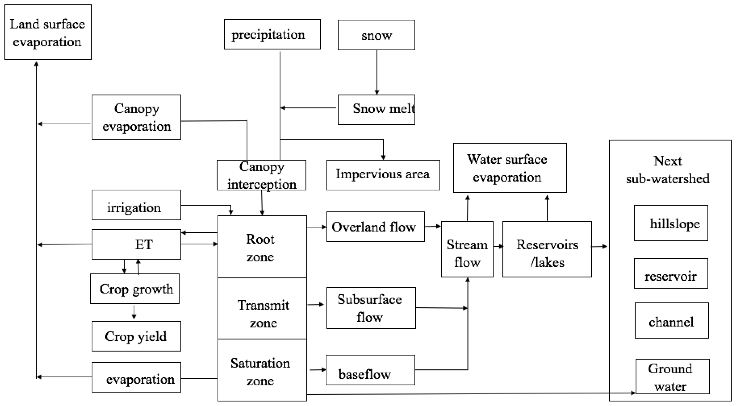
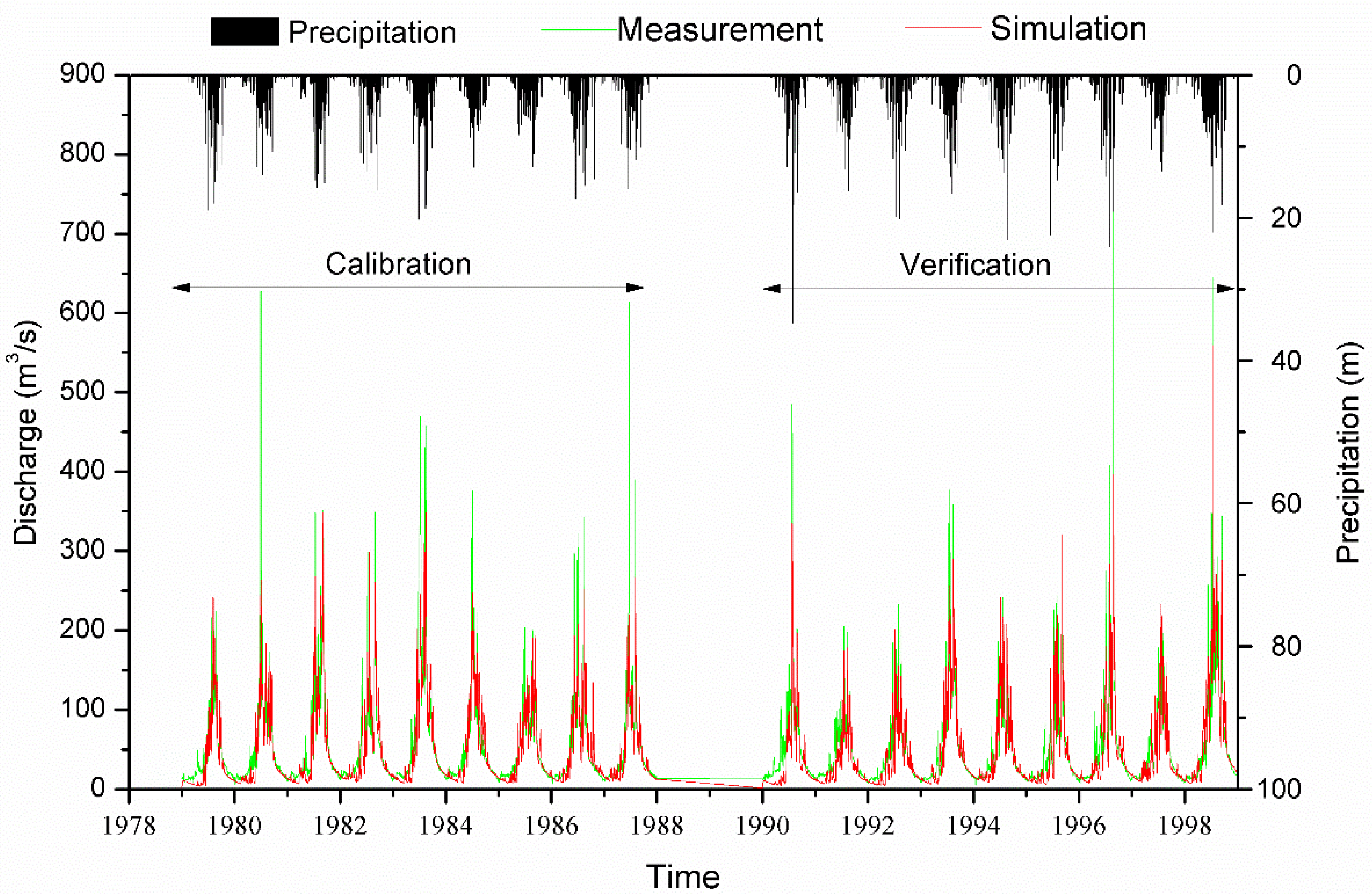
The upper reach locates in the semi-arid mountain area with runoff generated by the two mechanisms of intensity excess and saturation excess, therefore, HIMS is utilized to simulate the streamflow of the contributing area due to its structure of the combined runoff generation mechanisms. Simulated streamflow with HIMS model has greater predicting accuracy than those simulated with other models such as VIC and SWAT in the same study period. Water balance is closed in the study period for the upper reach with precipitation and snowmelt as the major water sources.

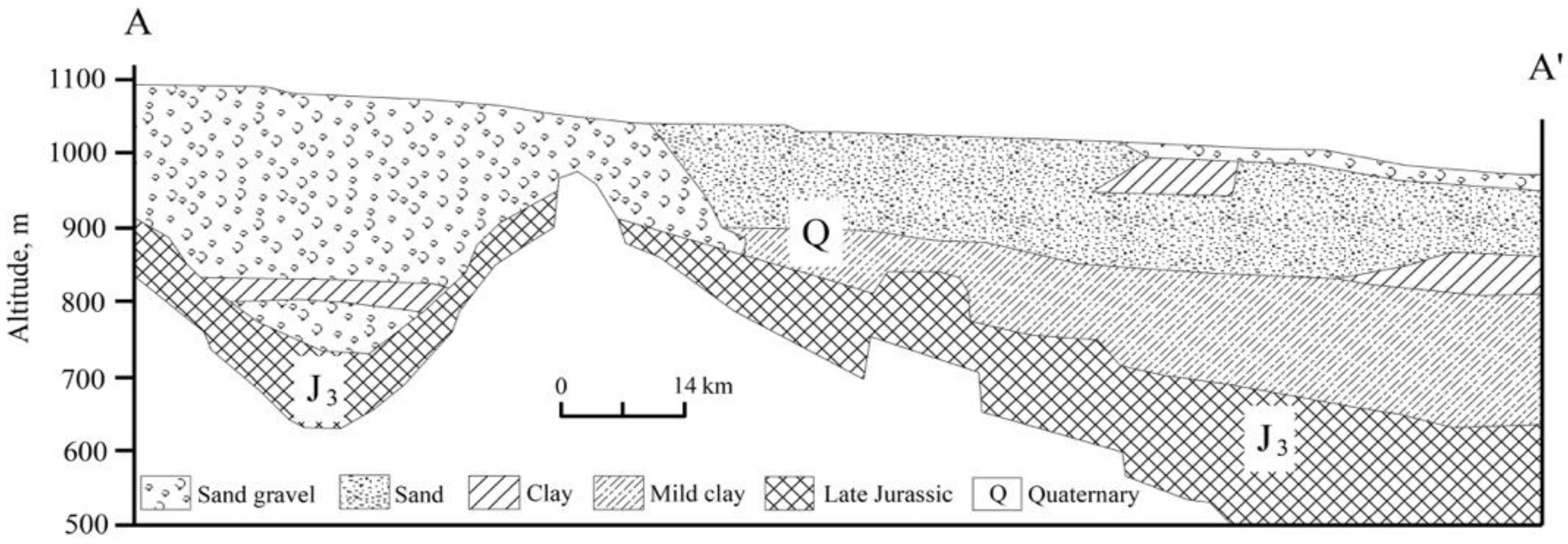
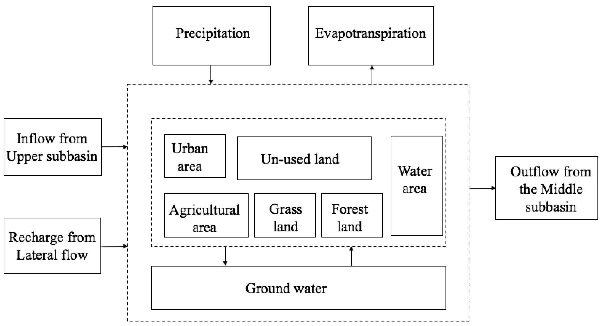
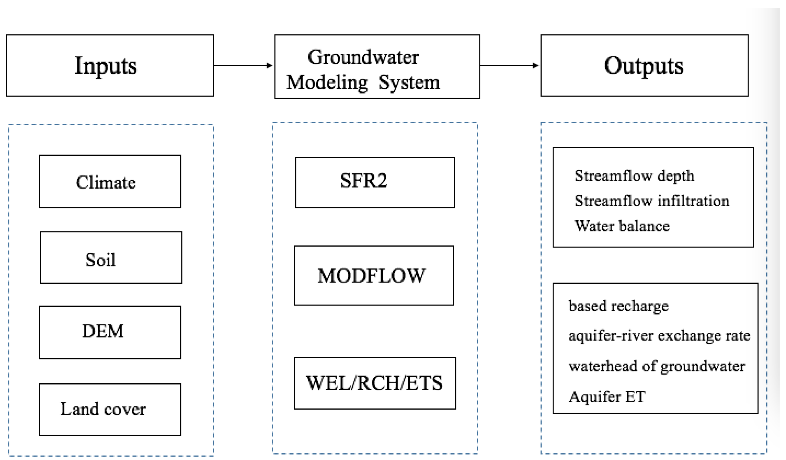
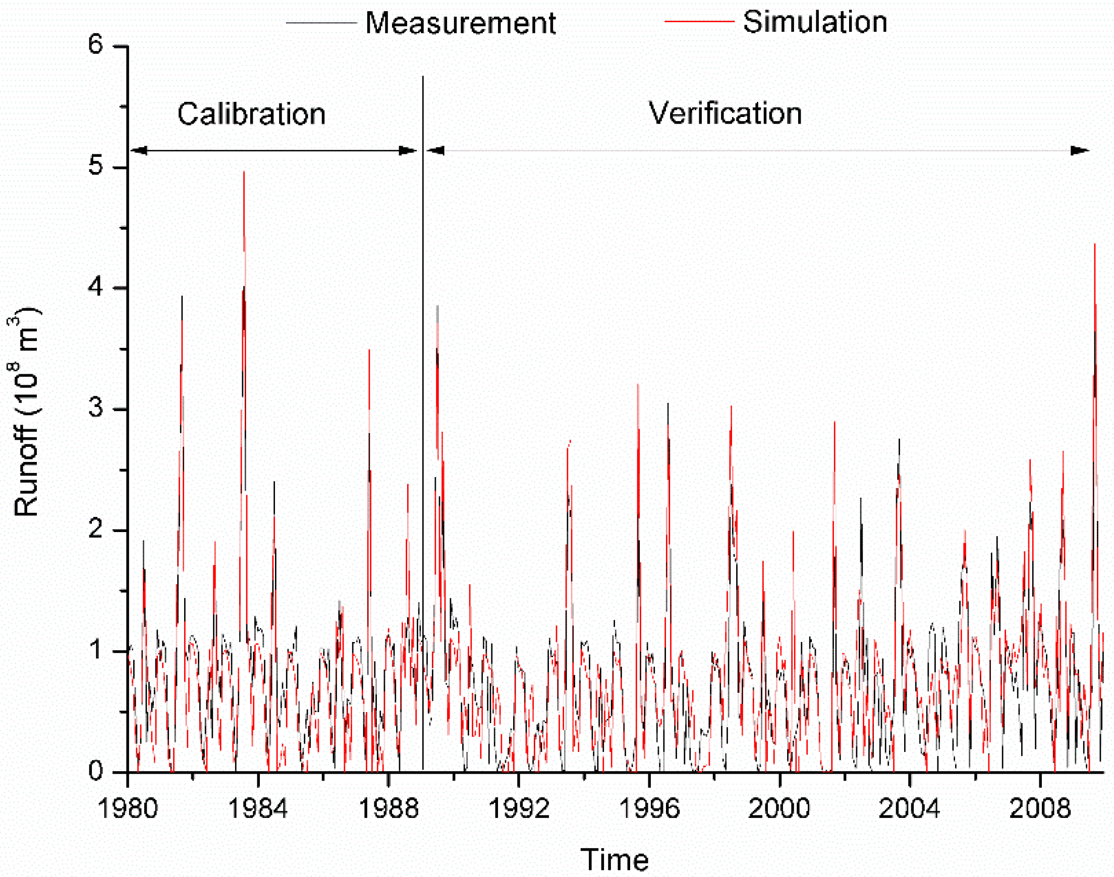
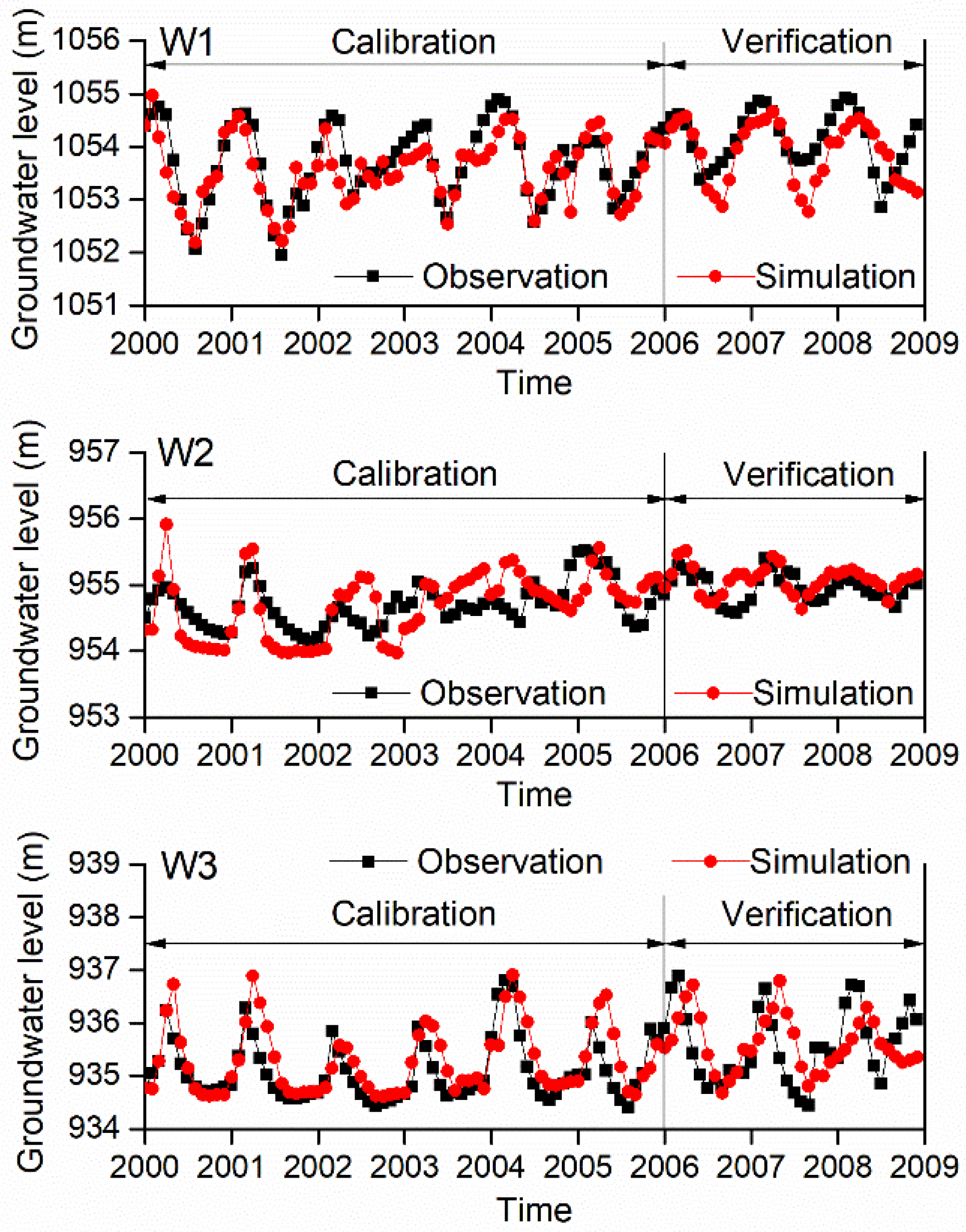
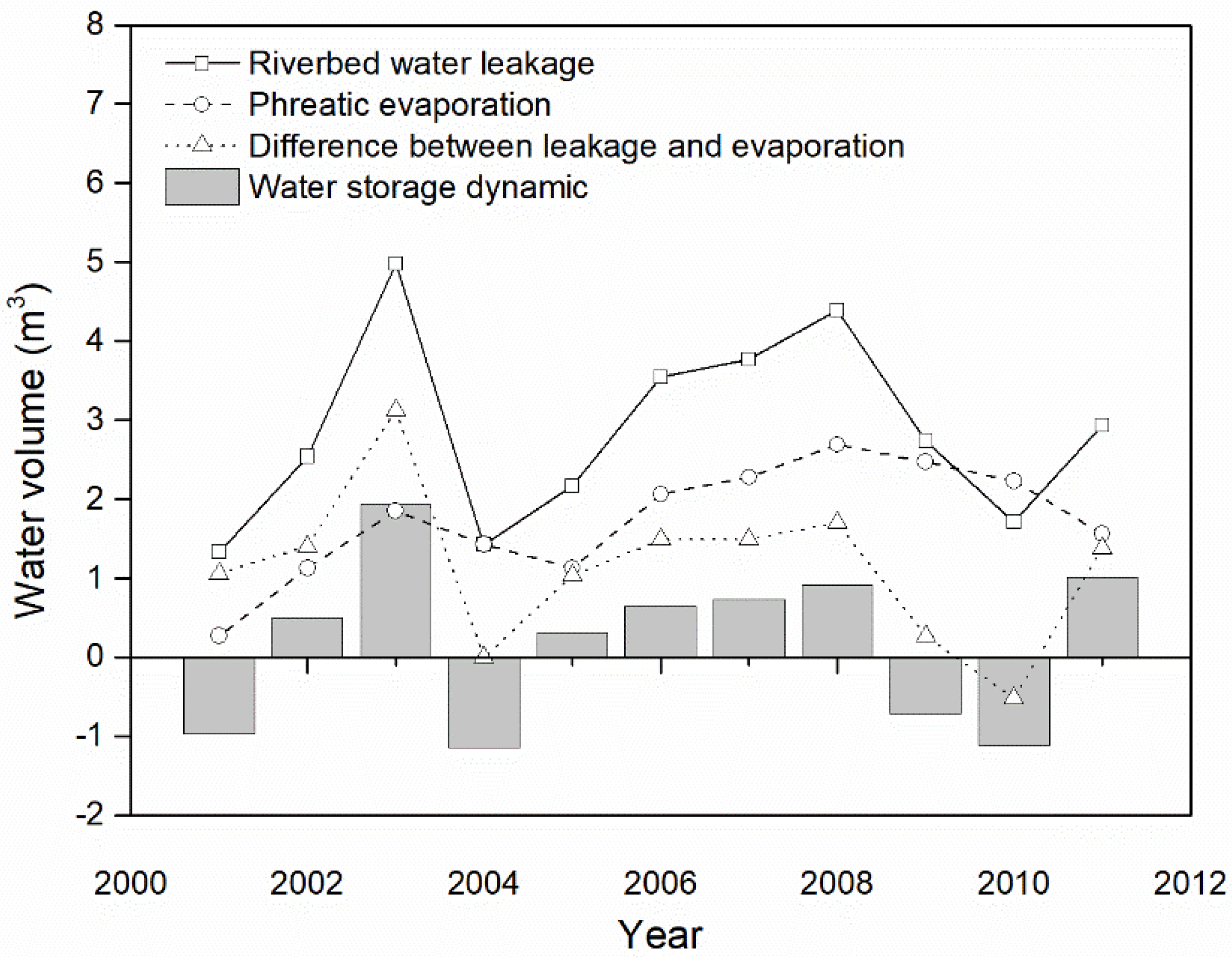
The middle reach is the dissipative area located in the arid area and a conceptual water balance model is utilized in simulating its streamflow accounting for the frequent interactions between the surface and subsurface flows under the impacts of the intensive human activities. Water balance is kept for the six land use types and the entire middle reach with the major inflow of precipitation and outflow of ET. More downstream flow can be expected through reducing ET and infiltration with effective irrigation methods and low water consuming crops. The lower reach is the other dissipative area located in the extreme arid climate area and the groundwater dynamics is well simulated with the GMS based on the statistical results in the calibration and validation periods for 15 wells. Water balance of the lower reach is kept in the study period between the inflow and outflow, even though the lower reach locates in the extreme arid area. Percolation and evaporation are identified as the key factors influencing the groundwater level, as evaporation decreases and percolation increases the groundwater level. The groundwater level over the entire lower reach keeps elevating at the average annual pace of 0.02 m due to the ecological division with negative water storage change values in dry years such as 2001, 2004, 2009, and 2010. The groundwater level increases by 0.04 m/year in the near-river channel area and decreases in the areas far away from the channels.

References

1. Wang, Z.G.; Wang, L.; Liu, C.M.; Li, J.; Liu, X.C. Development of a flexible hydrological informatics modeling system (HIMS). J. Hydrol. 2017. in review. [Google Scholar]
2. Sherman, L.K. Streamflow from Rainfall by the Unit Graph Method. Eng. News Rec. 1932, 108, 501–505. [Google Scholar]
3. Crawford, N.H.; Linsley, R.K. Stanford Watershed Model IV. Stanford, Digital Simulation in Hydrology; Technical Report No. 39; Department of Civil Engineering, University of California: Berkeley, CA, USA, 1966. [Google Scholar]
4. Williams, J.R.; LaSeur, W.V. Water yield model using SCS curve numbers. J. Hydraul. Div. 1976, 102, 1241–1253. [Google Scholar]
5. Zhao, R.J. The Xinanjiang model applied in China. J. Hydrol. 1992, 135, 371–381. [Google Scholar]
6. Freeze, R.A.; Harlan, R.L. Blueprint for a physically-based, digitally simulated hydrologic response model. J. Hydrol. 1969, 9, 237–258. [Google Scholar] [CrossRef]
7. Arnold, J.G.; Srinivasan, R.; Williams, J.R. Large area hydrologic modeling and assessment part I: Model development. J. Am. Water Resour. Assoc. 1998, 34, 73–89. [Google Scholar] [CrossRef]
8. Donigian, A.S., Jr.; Bicknell, B.R.; Imhoff, J.C. Hydrologic Simulation Program—FORTRAN. In Computer Models of Watershed Hydrology; Sirgh, V.P., Ed.; Water Resources Publications: Highlands Ranch, CO, USA, 1995; pp. 395–442. [Google Scholar]
9. Liang, X.; Lettenmaier, D.P.; Wood, E.F.; Burges, S.J. A simple hydrologically based model of land surface water and energy fluxes for general circulation models. J. Geophys. Res. Atmos. 1994, 99, 14415–14428. [Google Scholar] [CrossRef]
10. Tague, C. Chapter 7. Heterogeneity in Hydrological Processes: A terrestrial Hydrological Modeling Perspective. In Ecological Function in Heterogeneity Landscapes; Lovett, G.M., Jones, C.G., Turner, M.G., Weathers, C.K., Eds.; Springer: New York, NY, USA, 2005. [Google Scholar]
11. Arnold, J.G.; Williams, J.R.; Nicks, A.D.; Sammons, N.B. SWRRB, a Basin Scale Simulation Model for Soil and Water Resources Management; USDA-ARS Grassland, Soil and Water Research Laboratory: Temple, TX, USA, 1990; Volume 45, p. 142.
12. Woods, R.; Sivapalan, M.; Duncan, M. Investigating the representative elementary area concept: An approach based on field data. Hydrol. Process. 1995, 9, 291–312. [Google Scholar] [CrossRef]
13. Delfiner, P.; Delhomme, J.P. Optimum interpolation by kriging. In Display and Analysis of Spatial Data; Davis, J.C., McCullagh, M.J., Eds.; John Wiley: New York, NY, USA, 1973; pp. 96–114. [Google Scholar]
14. Xie, Z.H.; Su, F.H.; Liang, X.; Zeng, Q.C.; Hao, Z.C.; Guo, Y.F. Applications of a surface runoff model with Horton and Dunne runoff for VIC. Adv. Atmos. Sci. 2003, 20, 165–172. [Google Scholar]
15. Rigon, R.; Bancheri, M.; Formetta, G.; de Lavenne, A. The geomorphological unit hydrograph from a historical critical perspective. Earth Surf. Process Landf. 2016, 41, 27–37. [Google Scholar] [CrossRef]
16. Rinaldo, A.; Marani, A.; Rigon, R. Geomorphological dispersion. Water Resour. Res. 1991, 27, 513–525. [Google Scholar] [CrossRef]
17. Fread, D.L. Flow Routing. In Handbook of Hydrology; Maidment, D.R., Ed.; McGraw-Hill: New York, NY, USA, 1993; 10.3. [Google Scholar]
18. Huber, W.C.; Dickinson, R.E. Storm Water Management Model. User’s Manual Ver. IV; U.S. Environmental Protection Agency: Washington, DC, USA, 1988.
19. Tian, W.D.; Li, X.; Cheng, G.C.; Wang, X.; Hu, B.X. Coupling a groundwater model with a land surface model to improve water and energy cycle simulation. Hydrol. Earth System. Sci. 2012, 16, 4707–4723. [Google Scholar] [CrossRef] [Green Version]
20. Kim, W.N.; Yoo, M.C.; Won, S.; Arnold, J.G. Development and application of the integrated SWAT–MODFLOW model. J. Hydrol. 2008, 356, 1–16. [Google Scholar] [CrossRef]
21. Li, H.; Beldring, S.; Xu, C.Y.; Huss, M.; Melvold, K.; Jain, S.K. Integrating a glacier retrea model into a hydrological model—Case studies of three glacierised catchments in Norway an Himalayan region. J. Hydrol. 2015, 527, 656–667. [Google Scholar] [CrossRef] [Green Version]
22. Chen, Y.; Zhang, D.; Sun, Y.; Liu, X.; Wang, N.; Savenije, H. Water demand management: A case study of the Heihe River Basin in China. Phys. Chem. Earth 2005, 30, 408–419. [Google Scholar] [CrossRef]
23. Zhou, S.; Huang, Y.F.; Yu, B.F. Effects of human activities on the eco-environment in the middle Heihe River Basin based on an extended environmental Kuznets curve model. Ecol. Eng. 2015, 76, 14–26. [Google Scholar] [CrossRef]
24. Xie, Q. Regional Hydrogeological Survey Report of the People’s Republic of China (1:200,000): Ejina 2008, K-47-[24] [R]; Water Conservancy Department of Inner Mongolia: Inner Mongolia, China.
25. Wang, P. Shallow groundwater dynamics and its driving forces in extremely arid areas: A case study of the lower Heihe River in northwestern China. Hydrol. Process. 2014, 28, 1539–1553. [Google Scholar] [CrossRef]
26. Wen, X.; Wu, Y.; Su, J.; Zhang, Y.; Liu, F. Hydrochemical characteristics and salinity of groundwater in the Ejina Basin, Northwestern China. Environ. Geol. 2005, 48, 665–675. [Google Scholar] [CrossRef]
27. Owen, S.J.; Jones, N.L.; Holland, J.P. A comprehensive modeling environment for the simulation of groundwater flow and transport. Eng. Comput. 1996, 12, 235–242. [Google Scholar] [CrossRef]
28. Li, Y. Water Balance Analysis of the Middle Reach of the Heihe River Basin. Master’s Thesis, Chinese Academy Sciences, Beijing, China, 2016. [Google Scholar]
29. Hargreaves, G.H.; Asce, F.; Allen, R.G. History and Evaluation of Hargreaves Evapotranspiration Equation. J. Irrig. Drain. Eng. 2003, 129, 53–63. [Google Scholar] [CrossRef]
30. Liu, C.M.; Wang, G.T. The estimation of small-watershed peak flows in China. Water Resour. Res. 1980, 16, 881–886. [Google Scholar] [CrossRef]
31. Gill, M.A. Flood routing by the Muskingum method. J. Hydrol. 1978, 36, 353–363. [Google Scholar] [CrossRef]
32. McDonald, M.G.; Harbaugh, A.W. A Modular Three-Dimensional Finite-Difference Ground-Water Flow Model. In Techniques of Water-Resources Investigations, Book 6; U.S. Geological Survey: Reston, VA, USA, 1988. [Google Scholar]
33. Moriasi, D.N.; Arnold, J.G.; Van Liew, M.W.; Bingner, R.L.; Harmel, R.D.; Veith, T.L. Model evaluation guidelines for systematic quantification of accuracy in watershed simulations. Trans. ASABE 2007, 50, 885–900. [Google Scholar] [CrossRef]
34. Yang, X.; Xiong, Z. Runoff Simulation in the Upper Reaches of Heihe River Basin Based on the RIEMS–SWAT Model, 2016. Water 2016, 8, 455. [Google Scholar] [CrossRef]
35. He, R.; Pang, B.; Zhang, L.Y.; Shi, R. Uncertainty analysis of VIC model based on GLUE method. J. Beijing Norm. Univ. 2014, 50, 576–580. [Google Scholar]
36. Sang, Y.F.; Wang, Z.G.; Liu, C.M. The impact of changing enviroments on the runoff regime of the arid Heihe River Basin, China. Theor. Appl. Climatol. 2013. [Google Scholar] [CrossRef]
37. Li, F.; Zhang, L.H.; He, C.S. Analysis of agricultural land use change in the middle reach of the Heihe river basin, Northwest China. Environ. Res. Public Health 2014, 11, 2698–2712. [Google Scholar]
38. Wang, P.; Zhang, Y.C.; Yu, J.J.; Fu, G.B.; Ao, F. Vegetation dynamics induced by groundwater fluctuations in the lower Heihe River Basin, northwestern China. J. Plant Ecol. 2013, 4, 77–90. [Google Scholar] [CrossRef]
39. Zhao, Y.; Wei, Y.P.; Li, S.B.; Wu, B.F. Downstream ecosystem responses to middle reach regulation of river discharge in the Heihe River Basin, China. Hydrol. Earth Syst. Sci. 2016, 20, 4469–4481. [Google Scholar] [CrossRef]
Figure 1. The Contour of Heihe River Basin and the three reaches together with the meteorological stations and hydrological stations.
Water 10 00421 g001
Figure 2. The geological cross section of the Ejina Oasis area in the lower subbasin.
Water 10 00421 g002
Figure 3. HIMS model customization (Wang et al. [1]).
Water 10 00421 g003
Figure 4. The structure of the concept water balance model for the middle reach.
Water 10 00421 g004
Figure 5. The structure of the GMS for the lower reach.
Water 10 00421 g005
Figure 6. Monthly streamflow comparison between the simulations and observations in the calibration and validation periods of the upper reach at Yingluoxia station.
Water 10 00421 g006
Figure 7. Monthly streamflow comparison between the simulations and observations in the calibration and validation periods of the middle reach at Zhengyixia station.
Water 10 00421 g007
Figure 8. Comparisons between simulated and measured groundwater levels of three wells in the lower reach.
Water 10 00421 g008
Figure 9. Water storage dynamics of the lower reach from 2001 to 2011.
Water 10 00421 g009