Abstract
The characterization of flow in subsurface porous media is associated with high uncertainty. To better quantify the uncertainty of groundwater systems, it is necessary to consider the model uncertainty. Multi-model uncertainty analysis can be performed in the Bayesian model averaging (BMA) framework. However, the BMA analysis via Monte Carlo method is time consuming because it requires many forward model evaluations. A computationally efficient BMA analysis framework is proposed by using the probabilistic collocation method to construct a response surface model, where the log hydraulic conductivity field and hydraulic head are expanded into polynomials through Karhunen–Loeve and polynomial chaos methods. A synthetic test is designed to validate the proposed response surface analysis method. The results show that the posterior model weight and the key statistics in BMA framework can be accurately estimated. The relative errors of mean and total variance in the BMA analysis results are just approximately 0.013% and 1.18%, but the proposed method can be 16 times more computationally efficient than the traditional BMA method.
1. Introduction
Groundwater flow and contaminant transport are the key issues in the groundwater resources management. However, it is challenging to accurately predict the dynamic behavior of groundwater flow and the distribution of the pollutant. This can commonly be attributed to the insufficient knowledge to accurately understand the dynamic process of the groundwater system and the limited size of the error-prone measurement data to fully characterize the properties of the subsurface system. As such, stochastic methods have been developed to quantitatively solve the groundwater flow and solute transport problems under uncertainty [1,2,3]. The uncertainty associated with the groundwater modeling can arise from a variety of the factors, such as the mathematical model to represent the physical and chemical processes in the groundwater system, the initial and boundary conditions, the heterogeneity characterization of the hydrogeological parameters, and the static or dynamic observation data to constrain the groundwater model [4,5].
The overall uncertainty in the groundwater system can be categorized into two forms [5,6,7,8]. One is the aleatory uncertainty, which is the consequence of the stochastic nature of the groundwater system. It cannot be reduced by building a better model or collecting more data. Therefore, many efforts have been put into diminishing the other type of uncertainty—i.e., the so-called the epistemic uncertainty. This process is usually referred to as model calibration or inverse modeling [9]. The function of inverse modeling is to constrain the predictive uncertainty on the static data (e.g., the hydraulic conductivity measurements) or dynamic data (e.g., the hydraulic head or the concentration of the contaminants). Many inverse modeling methods have been proposed in the literature. The gradient-based inverse modeling methods have been developed in the non-linear regression framework. These methods require computation of the derivative of the objective function (a measure of the mismatch between the predictions and the observations) with respect to the model parameters, e.g., maximum likelihood estimation method [10] and pilot point method [11,12]. The adjoint-state method is commonly used in the gradient-based inverse modeling methods to alleviate the computational burden [13]. The ensemble- or sampling-based methods have been developed in a Bayesian updating framework. These methods run an ensemble of realizations to obtain the posterior distribution of the model parameters conditioning on the observations, such as Markov chain Monte Carlo (MCMC) method [14,15], ensemble Kalman filter method (EnKF) [16,17], and particle filter [18].
The aforementioned inverse modeling methods only take the parameter uncertainty and the measurement data uncertainty into account, which implicitly assumes that the underlying model structure is correct. In other words, only the parameter uncertainty and data uncertainty are propagated into the predictive uncertainty, and the model uncertainty is ignored since a single best model is used [19]. This is partially attributed to the fact that the parameter uncertainty and data uncertainty are relatively easily integrated into a Bayesian inference or non-linear regression framework. The concept of equifinality has been proposed by [20], which finds that the same observation dataset can fit several models equally well. Due to the complexity of the natural groundwater system, it tends to be interpreted with multiple models [21]. The generalized likelihood uncertainty estimator (GLUE) was developed to deal with the equifinality issue [22], and has been applied in groundwater flow and contaminant transport problems [23,24]. Even though the introduction of the GLUE method has a huge impact on the uncertainty assessment concerning the integration of all the plausible models, it suffers from the criticisms that GLUE is essentially an incoherent method and that subjective decisions are required in the implementation of this method [25,26,27]. As an alternative, Bayesian model averaging (BMA) is considered to be a rigorous Bayesian analysis framework that can account for the model uncertainty [28,29]. BMA and its maximum likelihood version have been used widely in hydrogeological research [21,30,31,32,33,34]. GLUE and BMA were integrated together by [35] in order to make GLUE more coherent with the Bayesian analysis framework.
One critical issue hindering the implementation of the multi-model analysis framework is computational effort. For a large-scale groundwater model with millions of numerical grid nodes, even one simulation outcome can be tedious to obtain. Due to the requirement of fully exploring the posterior predictive distribution, a large set of model evaluations must be performed in the multi-model analysis framework, which will indisputably aggravate the situation. The construction of the response surface for the original model has recently attracted more attention [36]. Polynomial chaos expansion is an efficient method to construct the response surface model by using an orthonormal polynomial basis. In this way, the original stochastic model can be approximated by a well-designed high-dimensional polynomial. Since the computation of the polynomial is much more efficient than the original simulation model, the computational efficiency of the ensemble-based stochastic methods can be greatly improved. Due to the high computational efficiency, it has been integrated with several ensemble-based inverse modeling methods, such as MCMC [37], ensemble Kalman filter [38,39], and bootstrap filter [40]. The response surface model can create a projection to represent the dependence of the model response on model parameters. Construction of the response surface model requires that the model parameters are statistically independent of each other. In the groundwater system, the hydrogeological properties (e.g., hydraulic conductivity and porosity) are spatially correlated and heterogeneous. The spatial distribution of the heterogeneous properties is characterized by a random field, where the spatial correlation can be described by geostatistical methods [41]. The Karhunen–Loeve expansion (KLE) can be used to convert the spatial correlated random field of the hydrogeological properties into independent uncorrelated random variables [42]. The evaluation of the polynomial coefficient of PCE (polynomial chaos expansion) approximation is important. A stochastic finite element method was developed in [43] to solve the PCE coefficients with Galerkin scheme, but it is a non-intrusive method which requires manipulation of the governing equation and the solution of a coupled set of deterministic equations. An intrusive method to obtain the PCE coefficient has been developed so that the governing equation can be treated as a black box, and any existing solver can be easily adopted. The probabilistic collocation method (PCM) is a non-intrusive method developed by [44] which uses the points of numerical evaluation of the Galerkin integral as collocation points [45,46]. However, the previous response-surface-based inverse modeling methods can only consider a single best model as mentioned before, and thus the model uncertainty has been ignored.
The novelty of this research is the integration of the probabilistic collocation method (PCM) into a Bayesian model averaging framework (BMA) in order to improve the computational efficiency and accuracy of the uncertainty quantification by considering model uncertainty in groundwater systems. In this paper, the heterogeneous random field of the hydraulic conductivity field is considered, and the conditional random field of hydraulic conductivity can be generated through conditional Karhunen–Loeve expansion (KLE) when the direct measurements of hydraulic conductivity are available. The consideration of the spatial heterogeneity of hydraulic conductivity renders the parameterization of the groundwater system to be associated with a high-dimensionality. To the authors’ knowledge, the performance of PCM-based response surface models with such high-dimensionally parameterized groundwater problems has been rarely studied in the context of multi-model Bayesian analysis.
The remainder of the paper is arranged as follows: (1) A computationally efficient multi-model analysis framework is proposed in Section 2, which contains the BMA method to deal with model uncertainty and the PCM method to establish a response surface model by using unconditional or conditional KLE approximation for the random hydraulic conductivity field and PCE approximation for the hydraulic head; (2) A synthetic test is designed to demonstrate the implementation of the proposed method in Section 3, and the efficiency and accuracy of the proposed method are evaluated by comparing the PCM-based BMA method with the traditional one that uses brute-force Monte Carlo simulation; (3) Conclusions are drawn based on the analysis results in Section 4.
2. Methods
In this section, the key methods for this research are introduced. The general mathematical form of the groundwater model is given first, the BMA method in groundwater modeling is then presented with hydraulic conductivity as model parameter and hydraulic head as prediction variable, and finally the PCM method for constructing the response surface model is demonstrated.
2.1. Governing Equations of Groudnwater Flow System
According to the continuity equation, the mathematical form of the transient groundwater flow in a saturated aquifer system can be described as [2]:
where is the hydraulic head in location ( for two-dimensional problem and for three-dimensional problem) at time , is the specific storage, and is the source (or sink) term. ( for two-dimensional problem and for three-dimensional problem) is the flow rate, and can be expressed by using Darcy’s law:
where is the hydraulic conductivity in different locations. The spatial distribution of is usually heterogeneous, and the heterogeneity can be described by using a geostatistical method where the logarithm of , , is assumed to be a multi-Gaussian stochastic process. In this case, the governing equation becomes a stochastic partial differential equation [3].
The initial associated with the groundwater system can be written as:
The boundary conditions (including Dirichlet boundary condition and Neumann boundary condition) associated with the groundwater system can be written as:
where is the prescribed head on the Dirichlet boundary , is the prescribed flux across the Neumann boundary , and is the outward unit vector normal to the boundary.
2.2. Bayesian Model Averaging Method
Different conceptualizations of hydrogeological conditions and groundwater flow processes can lead to different groundwater models (in this case, multiple interpretations of the hydrogeological heterogeneity characterization and sink/source term are considered, as will be shown in Section 3). Consider that a set of mutually independent groundwater models , where is the index for a postulated model and is the number of postulated models, can be postulated to simulate a prescribed groundwater system. The hydraulic head h can be consistently predicted through all the individual models in the postulated model set, then the predictive probability of hydraulic head conditioning on available data can be given as [28,29]:
where is the conditional predictive probability of the hydraulic head based on individual models, and is the posterior model weight. This equation indicates that the multi-model predictive probability is the summation of the predictive probability of individual models weighted by their posterior model weights.
The predictive mean in the multi-model context can be written as:
The predictive variance can be written as:
It can be found that the predictive variance is composed of (i.e., the within-model variance), and is the between-model variance.
According to Bayes’ rule, the posterior model weight can be written as:
where is the prior model probability. Its value can be assigned if expert opinions are available; otherwise, it can be assumed to follow a uniform distribution where each model is equally weighted. is the marginal likelihood of a model.
In this study, the hydraulic conductivity is considered as the sole uncertainty parameter, and the marginal likelihood can be written as:
where is the likelihood function. There are many types of likelihood measures, such as model efficiency likelihood function and Fuzzy likelihood function, but a Gaussian-type likelihood function is commonly used [35]:
where is the covariance matrix of hydraulic head measurements.
The evaluation of the integral in Equation (10) requires Monte Carlo simulations with a large number of parameter realizations to ensure the convergence. In some large-scale cases, even one prediction outcome takes a long time to run. The large parameter realizations set combined with the alternatively postulated model set may make the problem infeasible to solve, even with modern computational facility. It is urgent to develop a suitable algorithm to alleviate the computational burden. In the following subsections, the PCM-based response surface model is introduced to serve that purpose.
2.3. Unconditional and Conditional Karhunen–Loeve Expansion Methods
The Karhunen–Loeve expansion method can convert a correlated random function into a polynomial with independent and identically distributed Gaussian random variables [45,46]. Since the log hydraulic conductivity, , is heterogeneous and spatial correlated. The spatial correlation can be characterized with a known covariance function . The covariance function is bounded, symmetric, and positive definite; thus, it can be expanded as:
where are the spatial coordinates with the lag distance as , is the eigenvalue, and is the eigenfunction.
The eigenfunctions are orthogonal, and form a complete set. They satisfy the condition:
where is the Kronecker delta function.
The KLE of a zero-mean stochastic process can be expressed as:
where is the standard Gaussian random variable following the normal distribution and is the parameter in a probability space. Note that eigenvalues and eigenfunctions are deterministic terms. The unconditional random field can be generated by finding its eigenvalues and eigenfunctions.
The eigenvalues and eigenfunctions of the covariance function can be solved from the Fredholm equation:
If there are measurements , it may require the generation of random field conditioning on these measurements. The generation of the conditional random field can be achieved by conditional Kriging. The conditional Kriging covariance is [2]:
where are weighting functions, and the subscript c represents “conditional”.
The weighting function can be computed by using the following Kriging equations:
Similar to unconditional case, the conditional eigenvalues and eigenfunctions of the conditional covariance functions can be solved from the following Fredholm equation:
Once the eigenvalue and eigenfunction of the conditional covariance function are obtained, the conditional log hydraulic conductivity random field can be generated using:
In Equations (14) and (19) for the unconditional and conditional cases, the polynomials are known because the covariance function is known and the eigenvalues and eigenfunctions are solvable. Both equations are associated with infinite terms. In practice, the truncated KLE up to a desired accuracy with the first N largest eigenvalues can be used. The preserved energy of the random process is [47]:
2.4. Polynomial Chaos Expansion Method
The distribution of hydraulic head is usually non-Gaussian, and the covariance structure is unknown; thus, it cannot be expanded using the KLE method. A more general method called polynomial chaos expansion can be used [45,46]:
where is the deterministic coefficient, and the multivariate basis denotes the polynomial chaos of degree P with respect to N independent random variables .
The finite form of polynomial chaos of order P can be written more compactly:
where is a multi-index with the norm as in the set . is the compacted expression form of the multivariate polynomial basis function. , and there is one-to-one correspondence between and ; is the number of PCE terms determined by random input dimensionality and polynomial chaos up to degree :
The multivariate polynomial basis function can be constructed from the tensor product of univariate basis functions:
where is the polynomial of degree i in the j-th dimension.
For Gaussian random variables, the univariate basis can be Hermite polynomials [48]:
Other distribution types of random variables are also allowed in the generalized polynomial chaos method [48], and the polynomial basis can be selected from the hypergeometric polynomials of Askey scheme; e.g., the Legendre polynomial can be selected for uniform variables, and Laguerre polynomials can be selected for Gamma variables.
2.5. Probabilistic Collocation Method
The expansion coefficient for log hydraulic conductivity by using KLE method is known, but the coefficient in PCE for the hydraulic head is unknown. To obtain the coefficients, the probabilistic collocation method can be used, which is derived on the basis of weighted residual method. Denoting as the differential operator in Equation (1), the stochastic partial differential equation of groundwater flow model can be written as [44,46]:
If the hydraulic head is approximated by using PCE with finite terms in Equation (22), the residual can be computed as:
The minimization of residual in probability space yields:
where is the weight function and is the probability density function. In PCM, the weight function is chosen as the Dirac delta function:
The residual minimization equation in the integral form can be rewritten as:
This indicates that PCM does not require the residual function to be defined in the full probability space, and only needs to evaluate the value of the residual at the given collocation points. This results in a set of uncoupled equations to solve the coefficients in the PCE approximation for hydraulic head.
The selection of the collocation points is crucial to obtain the PCE coefficients accurately. Here, we adopt a heuristic method presented in [45]. The collocation points are chosen to take the roots of the higher-order Hermite polynomial. When the number of roots exceeds the number of required collocation points, the roots that are closer to the origin are selected due to its higher probability in a univariate normal distribution. The number of the collocation points shall be equal to the number of the unknown coefficients in PCE; i.e., the value of in Equation (23). With each set of collocation points , , we can construct a log hydraulic conductivity field by using KLE, and a corresponding hydraulic head field can be obtained by running the original groundwater model. The PCE coefficient, , can be solved by using linear regression:
Once the PCE coefficients of the hydraulic head are obtained, the response surface model is built, which means that we do not need to run the original groundwater model any more. The likelihood function in Equation (11) can then be evaluated as:
The predictive mean and variance of the hydraulic head in Equations (7) and (8) can be directly computed from the PCE coefficients:
In this way, all the terms in the multi-model analysis can be evaluated efficiently with the aid of the built response surface model of the hydraulic head. The efficiency and accuracy of the PCM-based multi-model analysis are demonstrated through comparison with the brute-force Monte-Carlo-based (MC) method. The flowcharts for PCM-based and MC-based multi-model analysis methods are presented in Figure 1 and Figure 2.
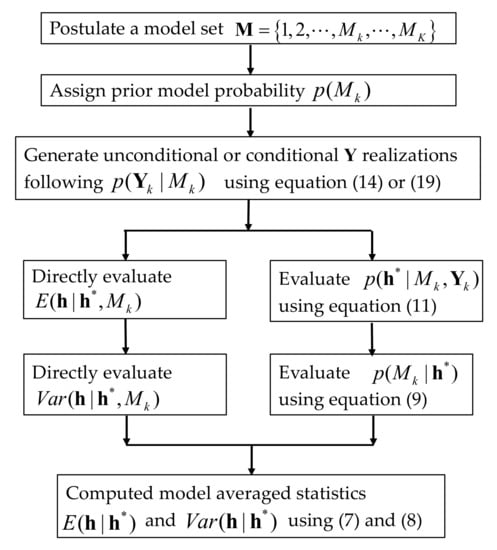
Figure 1.
Flowchart for Monte Carlo (MC)-based multi-model analysis.
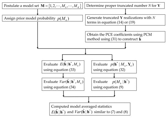
Figure 2.
Flowchart for probabilistic collocation method (PCM)-based multi-model analysis.
3. Results and Discussion
A two-dimensional saturated transient groundwater flow problem was designed to investigate the performance of the proposed PCM-based multi-model analysis method. In this section, the establishment of the reference model and alternative models, the detailed procedures to implement the proposed PCM-based multi-model analysis method, and the comparison results between PCM-based and MC-based multi-model analysis methods are presented.
3.1. Establishment of the Reference Model and Alternative Model Set
In the designed synthetic test, the domain was uniformly discretized into a 40 × 40 grid. Each cell had a square shape with a unit length (all quantities are given in consistent spatial length and temporal units, and the units for all the variables were ignored for concision). The zero-mean unconditional reference field of log hydraulic conductivity was generated using modified sequential Gaussian simulation code [41]. The reference variogram model used to generate the reference random field of log hydraulic conductivity was selected as the truncated power variogram model with Gaussian modes (TpvG) [32,49]:
where is the separation distance (lag) between any two points, is an upper cutoff scale proportional to domain size, is a Hurst scaling exponent—for this model . is variance, A is a coefficient so that the variance increases as a power of the upper cutoff scale, and is the incomplete gamma function. The corresponding integral scale is . Note that for a random field with constant finite variance , the relationship between variogram and covariance functions can be expressed as:
We set the parameters of the TpvG model equal to . The generated field can be found in Figure 3a. The reference flow model was designed with the left and right boundaries as the prescribed head ones and the upper and bottom boundaries as impervious ones. The prescribed head values were 10 (on the left) and 5 (on the right). A pumping well with a constant pumping rate of 5 was located at the center of the domain. The storage coefficient (i.e., the volume of water released from storage per unit decline in hydraulic head per unit area of the aquifer) was set to be 0.05. A rectangular recharge window with high permeability in the impermeable upper confining layer was used to reflect the effect of the geological discontinuity [34]. Its location can be found in Figure 3a. The flow problem was numerically solved using MODFLOW based on the reference log hydraulic conductivity field, and 20 time steps were simulated for the flow problem. The reference flow field at the last simulation step corresponding to the reference field is depicted in Figure 3b.
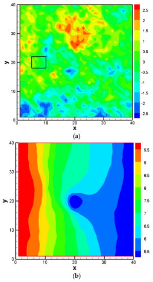
Figure 3.
Reference log hydraulic conductivity field and hydraulic head field distribution: (a) the reference log hydraulic conductivity field; (b) the reference hydraulic head field at the 20th time step. The black rectangle represents the location of the recharge window.
The obtained reference model was used to represent a typical real groundwater system in nature. However, in reality, the true groundwater system is unknown. To understand the system, we need to collect some samples from the true system. To simulate the sampling process, in this case, 10 log hydraulic conductivity data were randomly sampled from the reference field, and 20 randomly assigned monitoring wells provided dynamic hydraulic head data after the pumping well started pumping the groundwater out of the aquifer. The locations of the sampling process for log hydraulic conductivity data and hydraulic head data are shown in Figure 4. As discussed in Section 2, head observation data need to be perturbed with measurement errors. In this example, a measurement error with a magnitude of 1% of the observed hydraulic head value was added to perturb the observed hydraulic head data. These sampled data were considered as the only known information in the multi-model analysis.
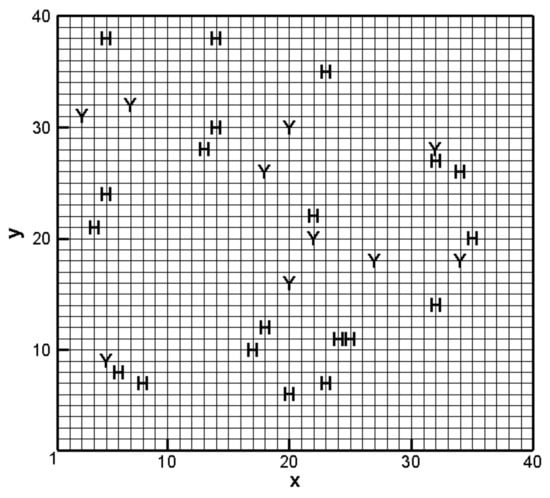
Figure 4.
Sampling locations of log hydraulic conductivity and hydraulic head. Y denotes the log hydraulic conductivity sampling locations and H represents the hydraulic head monitoring well location.
During the multi-model analysis, the model uncertainty needs to be considered; thus, a set of alternative models need to be postulated to analyze the obtained sampling information. Six alternative models are postulated in terms of the model uncertainty associated with the variogram types and the existence of the recharge window. The postulated model was intentionally selected in such a way that it was different from the reference one. The uncertainty associated with the existence of the recharge window lies in the fact that the geological discontinuity of the upper confining layer is difficult to detect by the current geophysical techniques. Several variogram models in geostatistics can characterize the correlation of the log hydraulic conductivity field. The selected variogram models are widely accepted exponential Gaussian and spherical models [41].
The exponential variogram can be written as:
The Gaussian variogram can be written as:
The spherical variogram can be written as:
The combination of three potential variogram models and two recharge window characterizations (existence or non-existence) resulted in six postulated models in the alternative model set. They are denoted as “Exp0” (exponential variogram without recharge window), “Exp1” (exponential variogram with recharge window), “Gau0” (Gaussian variogram without recharge window), “Gau1” (Gaussian variogram with recharge window), “Sph0” (spherical variogram without recharge window), and “Sph1” (spherical variogram without recharge window), respectively. All the settings of the problem design are summarized in Table 1.

Table 1.
Setting of the synthetic test to implement multi-model analysis.
3.2. Construction of PCM-Based Response Surface Model in BMA Multi-Model Analysis
The BMA multi-model analysis can be implemented in the standard manner with MC simulation [35] by using the above problem setting. The implementation procedures are summarized in Figure 1. However, it is well known that a large set of Y random realizations need to be generated in order to ensure the convergence of MC simulation results [50]. Here, after the convergence test introduced in [50], it was found that it required at least 10,000 realizations for each model to ensure the MC result convergence. Thus, it requires at least 60,000 groundwater simulation models to be run in order to obtain a reasonably converged result for the BMA multi-model analysis with six postulated alternative models. Even for a simple groundwater model such as the two-dimensional synthetic model here, it is tedious to obtain the results. Therefore, it is necessary to construct a response surface model to improve the efficiency of the BMA multi-model analysis.
The parameters in the three postulated variogram models need to be derived in order to conduct the geostatistical analysis. A sample variogram was obtained from 10 log hydraulic conductivity values, and the Levenberg–Marquardt non-linear regression algorithm was used to calibrate these three variogram models using the obtained the sample variogram. The calibration results can be found in Figure 5.
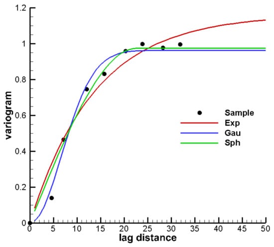
Figure 5.
Results of variogram model calibrations against sample variogram. Solid lines denote the calibrated variogram model curves, and black dots represent the sample variogram.
To construct the response surface model, we need to determine the proper truncated terms that can be retained in the KLE in Equation (12) for the unconditional case or (19) for the conditional case. Since there are 10 Y measurements, we need to use the conditional case. As mentioned in Section 2, the KLE to generate the conditional Y realizations is based on eigenvalues and eigenfunctions in the polynomial expansion. The generated conditional Y realization is mainly determined by the terms associated with the large eigenvalues. The computed eigenvalues for three calibrated variogram models were ranked from largest to smallest, and are depicted in Figure 6.
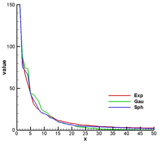
Figure 6.
Ranked eigenvalues for three postulated variograms.
It can be found that the first 30 eigenvalue terms were dominant in the KLE. The remaining eigenvalues can be safely ignored since they are too small to affect the final results of the KLE. The approach based on the visual inspection of the eigenvalue curve to determine the retained terms for KLE is effective, but rather qualitative.
A more quantitative way to determine the retained terms is to compute how much energy can be reserved for the corresponding retained terms by using Equation (20). The reserved energy curves are plotted in Figure 7. It can be found that if 85% of the total energy is deemed to be sufficiently reserved, then 26 terms need to be retained for the exponential variogram model, 18 terms for the Gaussian variogram model, and 12 terms for the spherical variogram model.
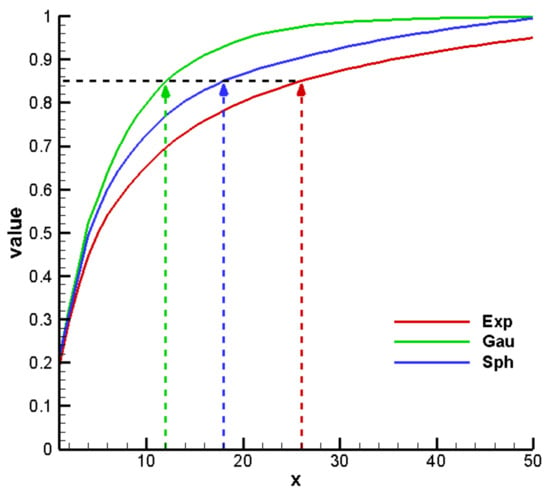
Figure 7.
Reserved energy curves for three postulated variograms.
After determining the proper number of the retained terms N in KLE for Y field, we need to select the proper polynomial order in PCE for hydraulic head. In this synthetic case, it can be shown that second order PCE (i.e., P = 2) was sufficient to approximate the hydraulic head. To obtain the collocations points, the roots of third-order univariate Hermite polynomial were used:
The roots of this univariate polynomial are . Therefore, the combination of these three roots can form a collocation point set for the PCM method. As a general rule, can be selected with priority since it is closer to the origin and has higher probability in a standard normal distribution. As mentioned in Section 2, the number of the collocation points is . For Exp0 and Exp1 model, it requires 325 collocation points. For Gau0 and Gau1 model, it requires 66 collocation points. For Sph0 and Sph1 model, it requires 153 collocation points. It can be inferred that the total number of forward groundwater modeling runs is 1088. Compared to the 60,000 forward runs in the MC-based multi-model analysis, the PCM-based analysis can reduce the number of model runs by a factor of 55. A huge amount of model evaluations can be saved, because once the response surface model is constructed, we do not need to evaluate the original groundwater model, but only to use the constructed response surface model to perform the multi-model analysis.
3.3. Comparison Results
To ensure the accuracy of the constructed response surface model, the posterior model probability of each model obtained through the PCM-based method was compared with that obtained through the MC-based method. The result is shown in Figure 8, from which it can be seen that PCM method could approximate the MC method very well in terms of the posterior model weight.
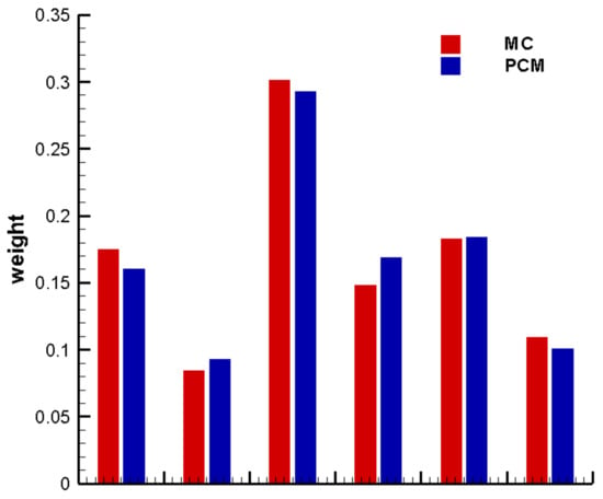
Figure 8.
Comparison of posterior model weight for each postulated model.
We then compared the obtained key statistics in the BMA multi-model analysis on the basis of the MC-based and PCM-based methods. The comparison results of the multi-model mean, within-model variance, between-model variance, and total variance are shown in Figure 9, Figure 10, Figure 11 and Figure 12, respectively. It can be found that the PCM-based analysis results with 1088 forward model runs could be as accurate as the MC-based results with 60,000 forward model runs.
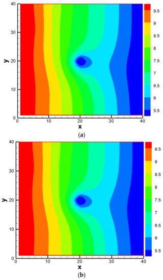
Figure 9.
Comparison of model averaged mean based on: (a) MC method; (b) PCM method.
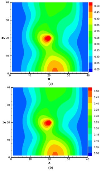
Figure 10.
Comparison of model averaged within-model variance based on: (a) MC method; (b) PCM method.
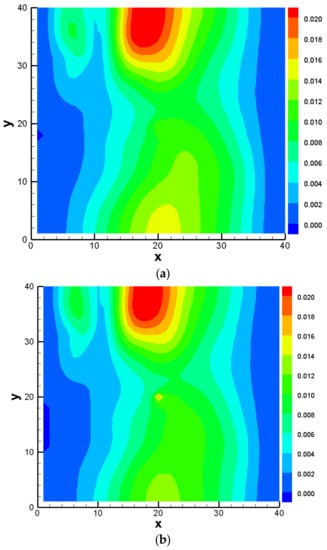
Figure 11.
Comparison of model averaged between-model variance based on: (a) MC method; (b) PCM method.
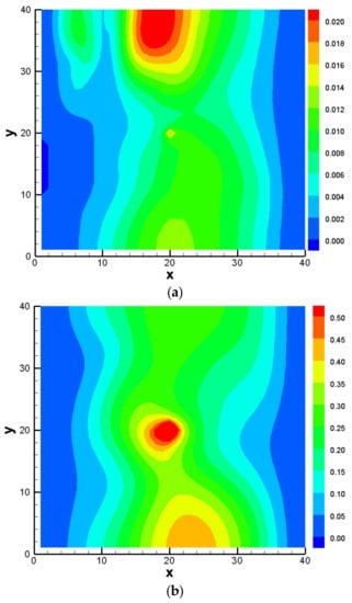
Figure 12.
Comparison of model averaged total variance based on: (a) MC method; (b) PCM method.
In addition to the visual inspection of the accuracy, we summarize the comparison results in terms of a scalar measure to get a more quantitative sense of accuracy. The scalar measurement is defined as the spatial average of the statistics () here, and it can be computed as:
where is the number of the grid nodes, and can be the value of multi-model mean, within-model variance, between-model variance, and total variance on the ith grid node. The comparison results are listed in Table 2. It can be found that the multi-model mean can be computed with the highest accuracy by using the PCM-based response surface model. This can be attributed to the fact that mean is a first-order statistical moment. For higher-order statistical moments, between-model variance had the largest error. However, the magnitude of the between-model variance was small relative to the within-model variance, and thus it did not significantly affect the total variance. The relative error was approximately 1%, which is acceptable. Overall, it is beneficial to use PCM-based response surface method to conduct BMA multi-model analysis.

Table 2.
Setting of the synthetic test to implement multi-model analysis.
In the previous subsection, the computational efficiency was compared in terms of the number of model evaluations. This is a theoretical measure of how much computational effort can be saved. Here, the computational time is further compared to show the computational efficiency. On the same computer with a 2.4 GHz CPU, the real computational time is demonstrated in Figure 13, where it can be found that the PCM-based method was almost 16 times more efficient than the MC-based one. The computational time was not proportionally reduced with the number of model evaluations, which is attributed to the fact that a large matrix inversion is required in Equation (31), and this step can be time-consuming. However, in this synthetic test, one forward run took less than 1 s. In a large-scale problem, a regional groundwater model can take hours to run. With the increase of the run time for each model evaluation, the time-consuming matrix inversion can become less significant and the computational efficiency can approach its theoretical measure.
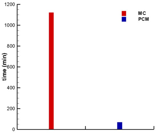
Figure 13.
Computational time for MC- and PCM-based multimodel analysis methods
4. Conclusions
A groundwater system is a complex natural system. Due to the data scarcity and limited knowledge, the characterization of groundwater systems tends to be interpreted with multiple models. Therefore, the model uncertainty may significantly affect the prediction of the groundwater system behavior. A Bayesian model averaging framework was developed to deal with the model uncertainty issue. However, the traditional BMA analysis is based on Monte Carlo simulation, which requires a large amount of forward model evaluations. To alleviate the computational burden, an efficient response surface model-based BMA analysis framework was proposed. The response surface model was constructed by using polynomial approximation, where the log hydraulic conductivity could be expanded into polynomials through Karhunen–Loeve method, hydraulic head could be expanded into polynomials through polynomial chaos method, and the PCE coefficients could be solved using probabilistic collocation method.
A two-dimensional synthetic groundwater flow problem was designed to demonstrate the procedures of the proposed analysis framework. The postulated multi-model set was developed based on the uncertainty of a variogram model to describe the heterogeneity of the hydraulic conductivity and geological discontinuity of the upper confining layer. To construct the polynomial response surface model, the proper retained terms in Karhunen–Loeve expansion for log hydraulic conductivity field and the order of polynomial in polynomial chaos expansion for hydraulic head need to be determined. In this case, the analysis shows that a polynomial with 26, 12, and 18 retained terms for exponential, Gaussian, and spherical variogram models and the second order is suitable to represent the original model. The accuracy of the proposed method was validated through comparison with the traditional method. The comparison results show that the computed posterior model probability and the key statistics (e.g., mean, within-model variance, between-model variance, and total variance) can all agree with those obtained through the traditional method very well. The relative errors of mean and total variance in the multi-model analysis were just 0.013% and 1.18%, respectively. By using the proposed method, the computational efficiency could be improved by 55 times in terms of the number of model evaluations and 16 times in terms of the CPU time.
Acknowledgments
This work is funded by the Science Foundation of China University of Petroleum-Beijing (Grant No. 2462014YJRC038), National Science and Technology Major Project (Grant Nos. 2016ZX05037003, 2016ZX05060002), China Postdoctoral Science Foundation (Grant No. 2016M591353), the Science Foundation of Sinopec Group (Grant No. P16058).
Author Contributions
Liang Xue performed the numerical test and wrote the paper; Cheng Dai designed the analysis framework; Yujuan Wu and Lei Wang analyzed the data.
Conflicts of Interest
The authors declare no conflict of interest.
References
- Gelhar, L.W. Stochastic subsurface hydrology from theory to applications. Water Resour. Res. 1986, 22, 135S–145S. [Google Scholar] [CrossRef]
- Zhang, D. Stochastic Methods for Flow in Porous Media: Coping with Uncertainties; Academic Press: Cambridge, MA, USA, 2001. [Google Scholar]
- Dagan, G.; Neuman, S.P. Subsurface Flow and Transport: A Stochastic Approach; Cambridge University Press: Cambridge, UK, 2005. [Google Scholar]
- Refsgaard, J.C.; Christensen, S.; Sonnenborg, T.O.; Seifert, D.; Højberg, A.L.; Troldborg, L. Review of strategies for handling geological uncertainty in groundwater flow and transport modeling. Adv. Water Res. 2012, 36, 36–50. [Google Scholar] [CrossRef]
- Gong, W.; Gupta, H.V.; Yang, D.; Sricharan, K., III; Hero, A.O. Estimating epistemic and aleatory uncertainties during hydrologic modeling: An information theoretic approach. Water Resour. Res. 2013, 49, 2253–2273. [Google Scholar] [CrossRef]
- Ross, J.L.; Ozbek, M.M.; Pinder, G.F. Aleatoric and epistemic uncertainty in groundwater flow and transport simulation. Water Resour. Res. 2009, 45, 641–648. [Google Scholar] [CrossRef]
- Sun, S.; Fu, G.; Djordjević, S.; Khu, S.T. Separating aleatory and epistemic uncertainties: Probabilistic sewer flooding evaluation using probability box. J. Hydrol. 2012, 420, 360–372. [Google Scholar] [CrossRef]
- Srinivasan, G.; Tartakovsky, D.M.; Robinson, B.A.; Aceves, A.B. Quantification of uncertainty in geochemical reactions. Water Resour. Res. 2007, 43, 497–507. [Google Scholar] [CrossRef]
- Sun, N.-Z. Inverse Problems in Groundwater Modeling; Springer: New York, NY, USA, 2013; Volume 6. [Google Scholar]
- Carrera, J.; Neuman, S.P. Estimation of aquifer parameters under transient and steady state conditions: 1. Maximum likelihood method incorporating prior information. Water Resour. Res. 1986, 22, 199–210. [Google Scholar] [CrossRef]
- Marsily, G.D.; Delay, F.; Gonçalvès, J.; Renard, P.; Teles, V.; Violette, S. Dealing with spatial heterogeneity. Hydrogeol. J. 2005, 13, 161–183. [Google Scholar] [CrossRef]
- Alcolea, A.; Carrera, J.; Medina, A. Pilot points method incorporating prior information for solving the groundwater flow inverse problem. Adv. Water Res. 2006, 29, 1678–1689. [Google Scholar] [CrossRef]
- Medina, A.; Carrera, J. Geostatistical inversion of coupled problems: Dealing with computational burden and different types of data. J. Hydrol. 2003, 281, 251–264. [Google Scholar] [CrossRef]
- Oliver, D.S.; Cunha, L.B.; Reynolds, A.C. Markov chain monte carlo methods for conditioning a permeability field to pressure data. Math. Geol. 1997, 29, 61–91. [Google Scholar] [CrossRef]
- Vrugt, J.A. Dream(d): An adaptive markov chain monte carlo simulation algorithm to solve discrete, noncontinuous, posterior parameter estimation problems. Hydrol. Earth Syst. Sci. 2011, 8, 3701–3713. [Google Scholar] [CrossRef]
- Chen, Y.; Zhang, D. Data assimilation for transient flow in geologic formations via ensemble kalman filter. Adv. Water Res. 2006, 29, 1107–1122. [Google Scholar] [CrossRef]
- Erdal, D.; Cirpka, O.A. Joint inference of groundwater-recharge and hydraulic-conductivity fields from head data using the ensemble kalman filter. Hydrol. Earth Syst. Sci. 2015, 12, 5565–5599. [Google Scholar] [CrossRef]
- Chang, S.-Y.; Chowhan, T.; Latif, S. State and parameter estimation with an sir particle filter in a three-dimensional groundwater pollutant transport model. J. Environ. Eng. 2012, 138, 1114–1121. [Google Scholar] [CrossRef]
- Zhou, H.; Gómez-Hernández, J.J.; Li, L. Inverse methods in hydrogeology: Evolution and recent trends. Adv. Water Res. 2014, 63, 22–37. [Google Scholar] [CrossRef]
- Beven, K.; Binley, A. The future of distributed models—Model calibration and uncertainty prediction. Hydrol. Process. 2010, 6, 279–298. [Google Scholar] [CrossRef]
- Neuman, S.P. Maximum likelihood bayesian averaging of uncertain model predictions. Stoch. Environ. Res. Risk Assess. 2003, 17, 291–305. [Google Scholar] [CrossRef]
- Beven, K.; Freer, J. Equifinality, data assimilation, and uncertainty estimation in mechanistic modelling of complex environmental systems using the glue methodology. J. Hydrol. 2001, 249, 11–29. [Google Scholar] [CrossRef]
- Binley, A.; Beven, K. Vadose zone flow model uncertainty as conditioned on geophysical data. Ground Water 2003, 41, 119–127. [Google Scholar] [CrossRef] [PubMed]
- Morse, B.S.; Pohll, G.; Huntington, J.; Castillo, R.R. Stochastic capture zone analysis of an arsenic-contaminated well using the generalized likelihood uncertainty estimator (glue) methodology. Water Resour. Res. 2003, 39, 377–380. [Google Scholar] [CrossRef]
- Montanari, A. Large sample behaviors of the generalized likelihood uncertainty estimation (glue) in assessing the uncertainty of rainfall-runoff simulations. Water Resour. Res. 2005, 41, 224–236. [Google Scholar] [CrossRef]
- Beven, K.J.; Smith, P.J.; Freer, J.E. So just why would a modeller choose to be incoherent? J. Hydrol. 2008, 354, 15–32. [Google Scholar] [CrossRef]
- Mcconnell, P. Hydrological forecasting uncertainty assessment: Incoherence of the glue methodology. J. Hydrol. 2006, 330, 368–381. [Google Scholar]
- Draper, D. Assessment and propagation of model uncertainty. J. R. Stat. Soc. Ser. B (Methodol.) 1995, 57, 45–97. [Google Scholar]
- Hoeting, J.A.; Madigan, D.; Raftery, A.E.; Volinsky, C.T. Bayesian model averaging: A tutorial. Stat. Sci. 1999, 14, 382–401. [Google Scholar]
- Poeter, E.; Anderson, D. Multimodel ranking and inference in ground water modeling. Ground Water 2005, 43, 597–605. [Google Scholar] [CrossRef] [PubMed]
- Nowak, W.; Barros, F.P.J.D.; Rubin, Y. Bayesian geostatistical design: Task-driven optimal site investigation when the geostatistical model is uncertain. Water Resour. Res. 2010, 46, 374–381. [Google Scholar] [CrossRef]
- Xue, L.; Zhang, D. A multimodel data assimilation framework via the ensemble kalman filter. Water Resour. Res. 2014, 50, 4197–4219. [Google Scholar] [CrossRef]
- Xue, L. Application of the multimodel ensemble kalman filter method in groundwater system. Water 2015, 7, 528–545. [Google Scholar] [CrossRef]
- Xue, L.; Zhang, D.; Guadagnini, A.; Neuman, S.P. Multimodel bayesian analysis of groundwater data worth. Water Resour. Res. 2015, 50, 8481–8496. [Google Scholar] [CrossRef]
- Rojas, R.; Feyen, L.; Dassargues, A. Conceptual model uncertainty in groundwater modeling: Combining generalized likelihood uncertainty estimation and bayesian model averaging. Water Resour. Res. 2008, 44, W12418. [Google Scholar] [CrossRef]
- Razavi, S.; Tolson, B.A.; Burn, D.H. Review of surrogate modeling in water resources. Water Resour. Res. 2012, 48, 7401. [Google Scholar] [CrossRef]
- Laloy, E.; Rogiers, B.; Vrugt, J.A.; Mallants, D.; Jacques, D. Efficient posterior exploration of a high-dimensional groundwater model from two-stage markov chain monte carlo simulation and polynomial chaos expansion. Water Resour. Res. 2013, 49, 2664–2682. [Google Scholar] [CrossRef]
- Li, W.; Oyerinde, A.; Stern, D.; Wu, X.H.; Zhang, D. Probabilistic collocation based kalman filter for assisted history matching—A case study. In Proceedings of the SPE Reservoir Simulation Symposium, The Woodlands, TX, USA, 21–23 February 2011. [Google Scholar]
- Dai, C.; Xue, L.; Zhang, D.; Guadagnini, A. Data-worth analysis through probabilistic collocation-based ensemble kalman filter. J. Hydrol. 2016, 540, 488–503. [Google Scholar] [CrossRef]
- Oladyshkin, S.; Class, H.; Nowak, W. Bayesian updating via bootstrap filtering combined with data-driven polynomial chaos expansions: Methodology and application to history matching for carbon dioxide storage in geological formations. Comput. Geosci. 2013, 17, 671–687. [Google Scholar] [CrossRef]
- Deutsch, C.; Journel, A. Gslib: Geostatistical Software Library and User’s Guide, 2nd ed.; Oxford University Press: Oxford, UK, 1998. [Google Scholar]
- Sarma, P.; Durlofsky, L.J.; Aziz, K.; Chen, W.H. Efficient real-time reservoir management using adjoint-based optimal control and model updating. Comput. Geosci. 2006, 10, 3–36. [Google Scholar] [CrossRef]
- Ghanem, R.G.; Spanos, P.D. Stochastic Finite Elements: A Spectral Approach; Springer: Berlin, Gremany, 1991; p. 224. [Google Scholar]
- Tatang, M.A.; Pan, W.; Prinn, R.G.; Mcrae, G.J. An efficient method for parametric uncertainty analysis of numerical geophysical models. J. Geophys. Res. Atmos. 1997, 102, 21925–21932. [Google Scholar] [CrossRef]
- Li, H.; Zhang, D. Probabilistic collocation method for flow in porous media: Comparisons with other stochastic methods. Water Resour. Res. 2007, 43, 6627–6632. [Google Scholar] [CrossRef]
- Liao, Q.; Zhang, D. Probabilistic collocation method for strongly nonlinear problems: 1. Transform by location. Water Resour. Res. 2013, 49, 7911–7928. [Google Scholar] [CrossRef]
- Chang, H.; Zhang, D. A comparative study of stochastic collocation methods for flow in spatially correlated random fields. Commun. Comput. Phys. 2009, 6, 509–535. [Google Scholar]
- Xiu, D.; Karniadakis, G.E. Modeling uncertainty in steady state diffusion problems via generalized polynomial chaos. Comput. Methods Appl. Mech. Eng. 2002, 191, 4927–4948. [Google Scholar] [CrossRef]
- Di Federico, V.; Neuman, S.P. Scaling of random fields by means of truncated power variograms and associated spectra. Water Resour. Res. 1997, 33, 1075–1085. [Google Scholar] [CrossRef]
- Ballio, F.; Guadagnini, A. Convergence assessment of numerical monte carlo simulations in groundwater hydrology. Water Resour. Res. 2004, 40, 285. [Google Scholar] [CrossRef]
© 2018 by the authors. Licensee MDPI, Basel, Switzerland. This article is an open access article distributed under the terms and conditions of the Creative Commons Attribution (CC BY) license (http://creativecommons.org/licenses/by/4.0/).