Sensitivity Analyses for Modeling Evolving Reactivity of Granular Iron for the Treatment of Trichloroethylene

Abstract

To better predict long-term performance of a remediation system, parameters of a numerical model should be constrained with care by calibrating with reliable experimental data. This study conducted sensitivity analyses for model parameters, which were shown to represent reasonably well the observed geochemical behaviors for the column experiments that evaluated evolving reactivity of granular iron for the treatment of trichloroethylene (TCE) resulting from precipitation of secondary minerals. The particular model parameters tested include iron corrosion rate, aragonite and Fe₂(OH)₂CO₃ precipitation rates, and proportionality constants for each mineral. For sensitivity analyses, a specific parameter was systematically changed, while other parameters were fixed at the values for the base case. The ranges of parameters tested were determined based on the previous modeling study. The results showed that the most important and sensitive model parameters were secondary mineral precipitation rates. Also, not only absolute precipitation rate for each mineral but also relative precipitation rates among different minerals were important for system performance. With help of sensitivity analysis, the numerical model can be used as a predictive tool for designing an iron permeable reactive barrier (PRB) and can provide implications for the long-term changes in reactivity and permeability of the system.

1. Introduction

Permeable reactive barriers (PRBs) using granular iron as a reactive material have been successfully applied for the removal of various contaminants in groundwater [1,2,3], and they are now accepted as one of the standard remediation options for contaminated groundwater [4,5].

While field demonstrations have shown that PRBs can be effective in the long term [1,6], concerns remain how long reactivity of iron and permeability of the systems can last under various geochemical conditions. Studies have shown that major geochemical components, such as calcium and carbonate, and oxidants, such as nitrate and chromate, can negatively affect the reactivity and permeability of iron PRBs [7,8,9].

Laboratory [10,11], field [1,6,12], and reactive transport modeling [13,14,15] experiments have been conducted to evaluate the reactivity and permeability of iron PRBs. In particular, reactive transport modeling can be used to assess various geochemical conditions without having extensive labor and cost for changing various conditions for laboratory and field tests. Given reasonable model parameter sets, the established model can be used to predict future performance of the systems.

Jeen et al. [16], in particular, showed that reactive transport modeling can be effective to demonstrate the geochemical patterns observed over time in a column experiment. A multi-component reactive transport model was modified to reflect the evolving reactivity of iron caused by precipitation of secondary carbonate minerals on the iron surfaces. The key consideration of the model was to update the reactive surface area of the iron, as geochemical conditions changed temporally and spatially over time. The modified model has since been successfully used to demonstrate the observed behaviors of geochemistry over time for laboratory experiments [8,17,18,19] and field tests [20].

One of the remaining concerns about simulating long-term performance of iron PRBs using a model, as an example of Jeen et al. [16], is the predictive capability of the model with regard to the sensitivity of model parameters. By evaluating more sensitive model parameters for predictive simulation, one can spend more effort to get reliable model parameter values to improve predictability. Thus, the purposes of this study were to evaluate the sensitivity of model parameters for modeling evolving reactivity of iron, to identify more important parameters to predict the long-term performance of iron PRBs, and thus to provide insights for evolution of the systems with regard to changes in reactivity and permeability. This study conducted sensitivity analysis for model parameters, which were shown to be important to represent the geochemical evolution of a laboratory column experiment.

2. Methods

2.1. Model

The numerical model MIN3P [21] was developed for multi-component reactive transport simulations in variably saturated porous media. The governing equations were discretized using a locally mass conservative finite volume method and were linearized by a global implicit solution method [22,23]. The formulation of the model was based on a partial equilibrium approach [22,24,25], allowing inclusion of kinetic limitations, which are essential for adequate description of groundwater treatment by PRB systems.

Previous studies showed that the reaction of granular iron and groundwater causes precipitation of secondary minerals, and the precipitation front migrates as the reactivity of iron is decreasing because of the deposition of secondary minerals on iron surfaces [26,27]. In order to adequately reproduce the changes in iron reactivity, it is key to incorporate the evolving reactivity of the iron into the kinetic formulations in MIN3P. Inclusion of the evolving reactivity of iron was realized by updating the reactive surface area of the iron based on the laboratory-derived relationship between secondary mineral volume fraction and reactive surface area of iron [16].

In MIN3P, the rate expression for dissolution-precipitation of minerals is described as follows:

$$R_i^m=-k_{eff,i}\cdot S_i\left(1-\frac{{\mathrm{IAP}}_i^m}{K_i^m}\right)$$

(1)

where $k_{\mathrm{eff},i}$ is the effective rate constant for the dissolution of mineral phase i (mol L⁻¹ H₂O s⁻¹), $S_i$ is the reactive surface area of mineral phase i (m² L⁻¹ bulk), and ${\mathrm{IAP}}_i^m$ and $K_i^m$ are the ion activity product and the corresponding equilibrium constant for mineral dissolution-precipitation reactions, respectively. The two important secondary minerals identified by X-ray diffraction (XRD) [28] and tested for the sensitivity analyses in this study are aragonite and Fe₂(OH)₂CO₃.

The extent to which the accumulation of an individual mineral phase affects the reactivity of iron is represented by:

$$S(x,t)=S_0\cdot exp\left(-{\displaystyle \sum _i{\mathsf{\alpha }}_i\hspace{0.17em}{\phi }_i(x,t)}\right)$$

(2)

where $S(x,t)$ is the reactive surface area of the iron at a specific location along the flow path and time (m² iron L⁻¹ bulk), $S_0$ is the initial reactive surface area of iron (m² iron L⁻¹ bulk), ${\mathsf{\alpha }}_i$ is the proportionality constant for mineral phase i, and ${\phi }_i(x,t)$ is the volume fraction of the mineral phase i at a specific location and time (-). The proportionality constant for each mineral phase represents the extent to which a particular mineral phase contributes to the reactivity loss of iron.

The reaction rate for trichloroethylene (TCE) degradation is represented by:

$$\frac{\mathrm{d}\left[\mathrm{TCE}\right]}{\mathrm{dt}}=-k_{\mathrm{SA}–\mathrm{TCE}–{\mathrm{Fe}}^0}\cdot S(x,t)\frac{\left[\mathrm{TCE}\right]}{K_{1/2}+\left[\mathrm{TCE}\right]}$$

(3)

where $k_{\mathrm{SA}–\mathrm{TCE}–{\mathrm{Fe}}^0}$ is the rate constant of TCE normalized to iron surface area (mol m^-2 iron s⁻¹), $\left[\mathrm{TCE}\right]$ is the concentration of TCE (mol L⁻¹ H₂O), and $K_{1/2}$ is the half-saturation constant (mol L⁻¹ H₂O), which corresponds to the TCE concentration at half-maximum transformation rate. It was considered that about 5% of TCE is degraded by hydrogenolysis to cis-1,2-dichloroethylene (cis-1,2-DCE) and the remaining 95% is degraded to ethene via β-elimination [16]. The rate expression for iron corrosion by water is represented by:

$$R_{{\mathrm{H}}_2\mathrm{O}–{\mathrm{Fe}}^0}=-max\hspace{0.17em}\left\{\left[k_{\mathrm{SA}–{\mathrm{H}}_2\mathrm{O}–{\mathrm{Fe}}^0}\cdot S(x,t)\hspace{0.17em}\left(1-\frac{{\mathrm{IAP}}_{{\mathrm{H}}_2\mathrm{O}–{\mathrm{Fe}}^0}}{K_{{\mathrm{H}}_2\mathrm{O}–{\mathrm{Fe}}^0}}\right)\right],\hspace{0.17em}0\right\}$$

(4)

where $k_{\mathrm{SA}–{\mathrm{H}}_2\mathrm{O}–{\mathrm{Fe}}^0}$ is the rate constant of iron corrosion normalized to iron surface area (mol m⁻² iron s⁻¹), ${\mathrm{IAP}}_{{\mathrm{H}}_2\mathrm{O}–{\mathrm{Fe}}^0}$ is the ion activity product, and $K_{{\mathrm{H}}_2\mathrm{O}–{\mathrm{Fe}}^0}$ is the equilibrium constant.

In MIN3P, porosity and hydraulic conductivity are updated to reflect the changes during the simulation as secondary minerals precipitate and iron dissolves. The hydraulic conductivity was updated based on a normalized version of the Kozeny-Carmen relationship. The details of the model description and model validation processes can be found in Jeen et al. [16], and description of the column test, to which the model was applied, can be found in Jeen et al. [28]. The sensitivity analyses in this study were performed for column D of Jeen et al. [16,28].

2.2. Model Parameters

Based on the observed geochemical changes in the column, the following 11 aqueous components were included for the expression of all chemical reactions: Ca²⁺, Cl⁻, CO₃²⁻, Fe²⁺, Fe³⁺, H⁺, H₂(aq), TCE, cis-1,2-DCE, vinyl chloride (VC), ethene, and H₂O. A total of 12 aqueous complexes were also included for appropriate determination of mineral solubilities. The equilibrium constants were taken from the databases of MINTEQA2 [29] and WATEQ4F [30].

To represent the column system, one-dimensional discretization was used, with a spatial discretization interval of 0.01 m for the 0.5 m long column, giving a total of 51 grid points. The flow system was modeled as a fully saturated system with a second type (specified flux) boundary at the influent end and first type (specified head) boundary at the effluent end. The flow rate (1.38 × 10⁻⁵ m s⁻¹) at the influent of the column was used for the specified flux at the influent end, and zero hydraulic head was specified at the effluent end. Zero hydraulic head for the entire domain was specified as the initial condition for the flow simulation.

A diffusion coefficient of 1.5 × 10⁻⁹ m² s⁻¹ [31] and longitudinal dispersivity of 9.9 × 10⁻⁴ m were used as the transport parameters. Boundary conditions for reactive transport were the third type (specified mass flux) at the influent end and the second type (free exit) at the effluent end. The measured aqueous concentrations and pH of the source water for each column were used as the influent chemical compositions. The initial condition for reactive transport, several orders of magnitude lower concentrations for each constituent, relative to the expected concentrations for the simulation, were specified in the entire domain. The detailed input parameters for the column test are summarized in

Table 1. Input parameters used in the simulation.

Model Input Parameter	Value
Column length (m)	0.50
Fe0 volume fraction (-)	0.49
Porosity (-)	0.51
Hydraulic conductivity (m s−1)	3.49 × 10−5
Diffusion coefficient (m2 s)	1.5 × 10−9
Longitudinal dispersivity (m)	9.9 × 10−4
Running time (days)	410
Flow rate (m s−1)	1.38 × 10−5
pH	6.66
Ca2+ (mol L−1)	5.0 × 10−3
CO3 Total (mol L−1)	1.57 × 10−2
TCE (mol L−1)	7.6 × 10−5

.

2.3. Sensitivity Analysis

For constraining the model parameters in Jeen et al. [16], adjustment of parameters was conducted to fit overall profiles over time, not to fit a single profile at a specific time. As a result, each of the model’s parameters had some ranges between different columns. The iron corrosion rate, aragonite and Fe₂(OH)₂CO₃ precipitation rates, and proportionality constants for each mineral were those with some ranges, and thus were parameters tested with sensitivity analyses in this study.

One set of model parameters, which provided the best fit to the data of column D, was selected as the base case for the sensitivity analyses. In Jeen et al. [31], column D received the highest concentration of aqueous calcium carbonate, showed the highest measured iron corrosion rate, and thus showed the fastest passivation of the iron over time [31]. Therefore, any changes in the model parameters could be reflected most sensitively to the modeling results.

For sensitivity analyses, a specific parameter was systematically changed, while other parameters were fixed at the values for the base case. The parameter values for the base case and the range tested for each parameter are shown in

Table 2. The parameter values for the base case and range tested for each parameter.

Parameter		Base Case	Sensitivity Analysis
Initial reactive surface area (m2 iron L−1 bulk)		8.37 × 103	Fixed
log $k_{SA–TCE–F{e}^o}$ a (mol m−2 iron s-1)		−10.95	Fixed
$K_{1/2}$b (mol L−1 H2O)		1.83 × 10−5	Fixed
log $k_{SA–H_{2}O–F{e}^0}$ c (mol m−2 iron s−1)		−9.90	−50%, −20%, +20%, +50%
log $k_{\mathrm{eff},i}$ d (mol L−1 H2O s−1)	CaCO3(s) (aragonite)	−6.93	×1/10, ×1/5, ×5, ×10
	Fe2(OH)2CO3(s)	−9.75	×1/10, ×1/5, ×5, ×10
${\mathsf{\alpha }}_1$e (for aragonite)		55	−50%, −20%, +20%, +50%
${\mathsf{\alpha }}_2$f (for Fe2(OH)2CO3(s))		2	−100%, −50%, +50%, +100%

Notes: ^a The trichloroethylene (TCE) rate constant normalized to iron surface area; ^b Half-saturation constant; ^c The iron corrosion rate constant normalized to iron surface area; ^d The effective rate constant for the dissolution of mineral phase i; ^e The proportionality constant for aragonite; ^f The proportionality constant for Fe₂(OH)₂CO₃(s).

.

3. Results and Discussion

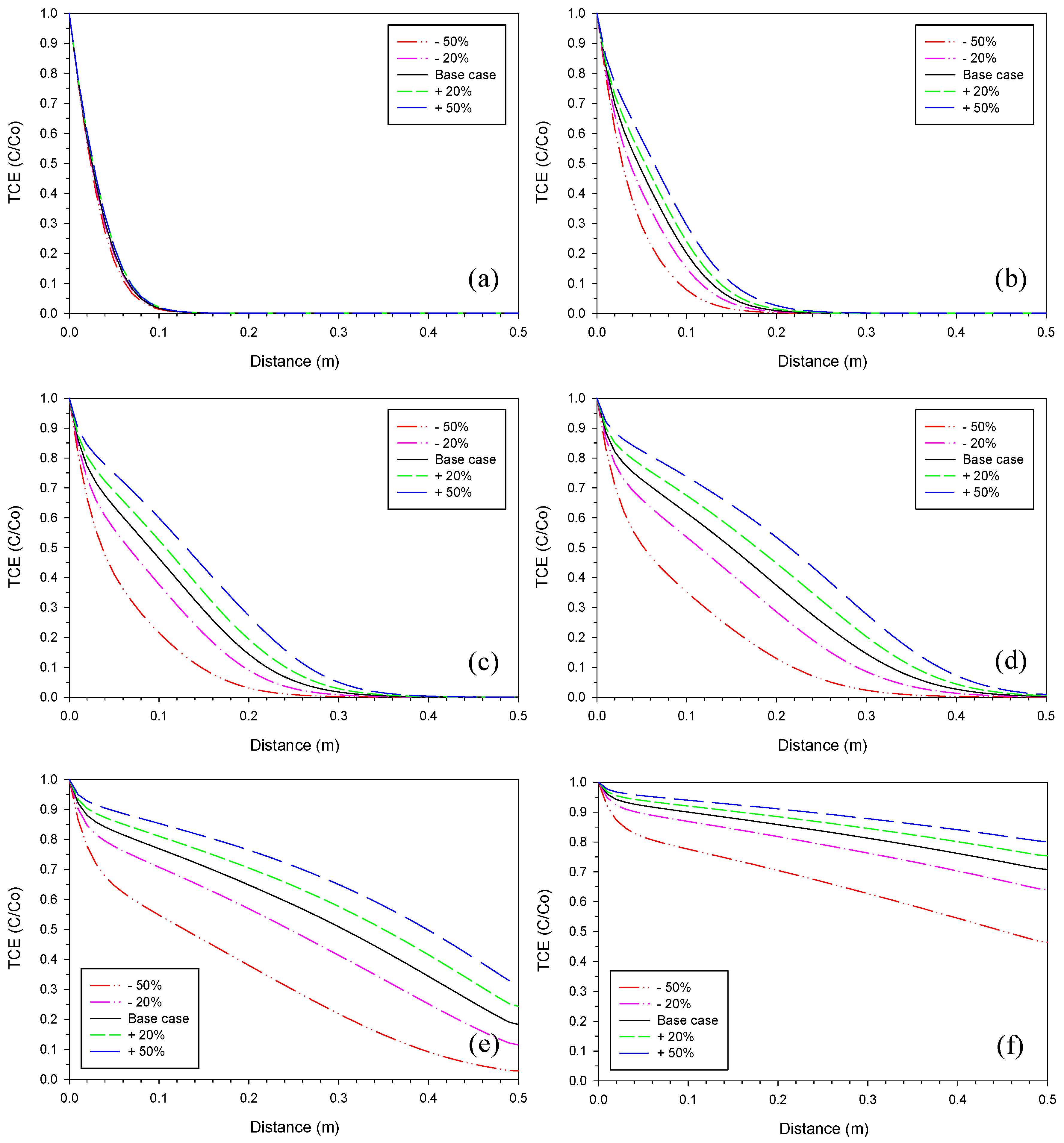
3.1. Iron Corrosion Rate

The range selected for the initial iron corrosion rate was +/−20%, +/−50% from the base case. The fitted iron corrosion rates were generally very close to the measured maximum iron corrosion rates [16]. Therefore, it was considered that the selected range for sensitivity analyses covers the possible changes induced by differences in the initial iron corrosion rate. Figure 1 shows the effect of the iron corrosion rate on the TCE profiles at different times. The deviations from the base case increased with time, approaching a maximum on Day 164. However, the effect leveled off at later times (Figure 1f) because of the exponential nature of the reactivity loss (Equation (2)).

With regard to mineral precipitation, when some amount of aragonite had accumulated, further increase in precipitation did not affect the reactivity to the same extent as the previous increase. The shape of accumulating aragonite did not change over time for different values of iron corrosion rate, but the amount of aragonite was proportional to the values of the iron corrosion rate (Figure 2).

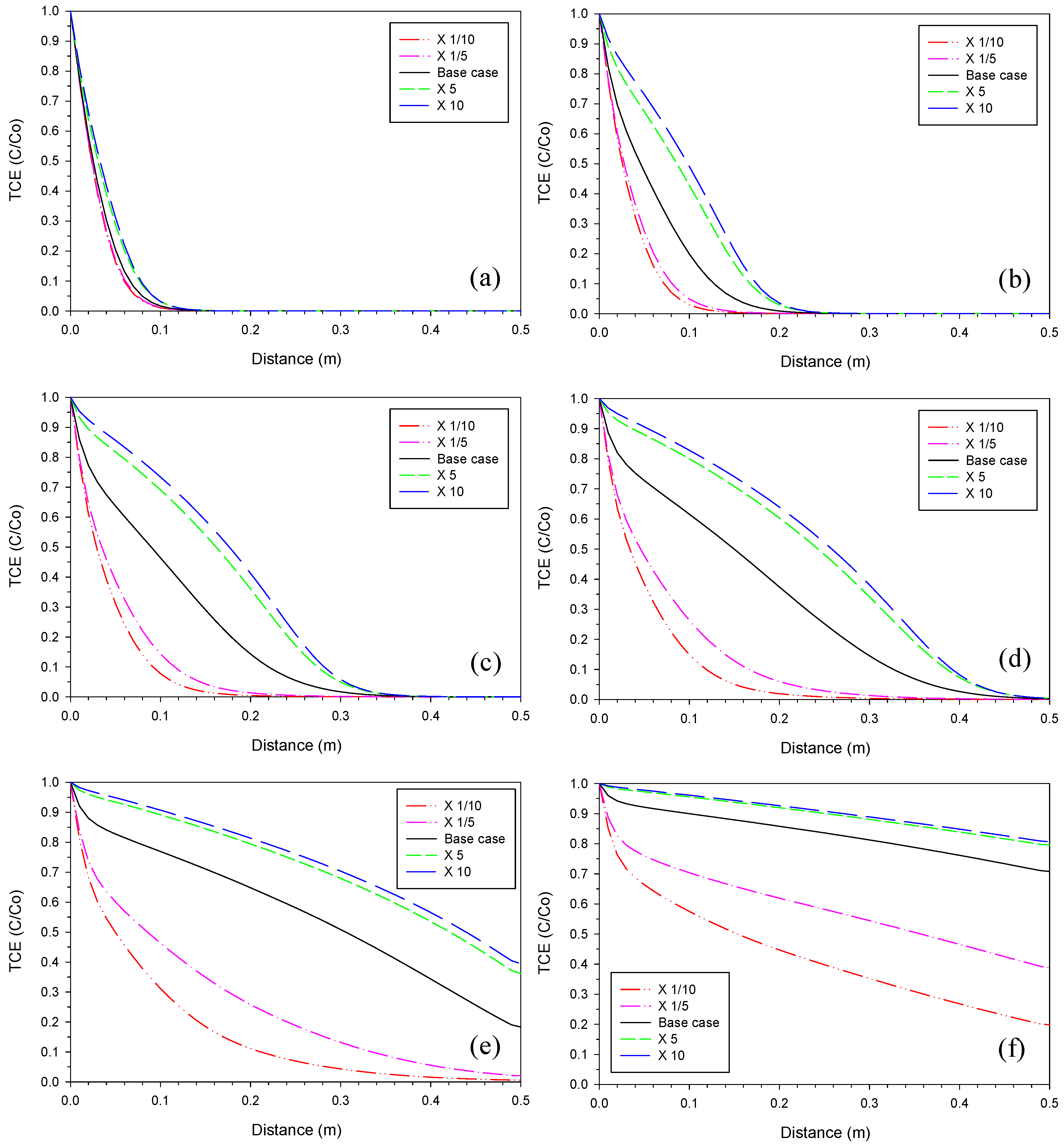
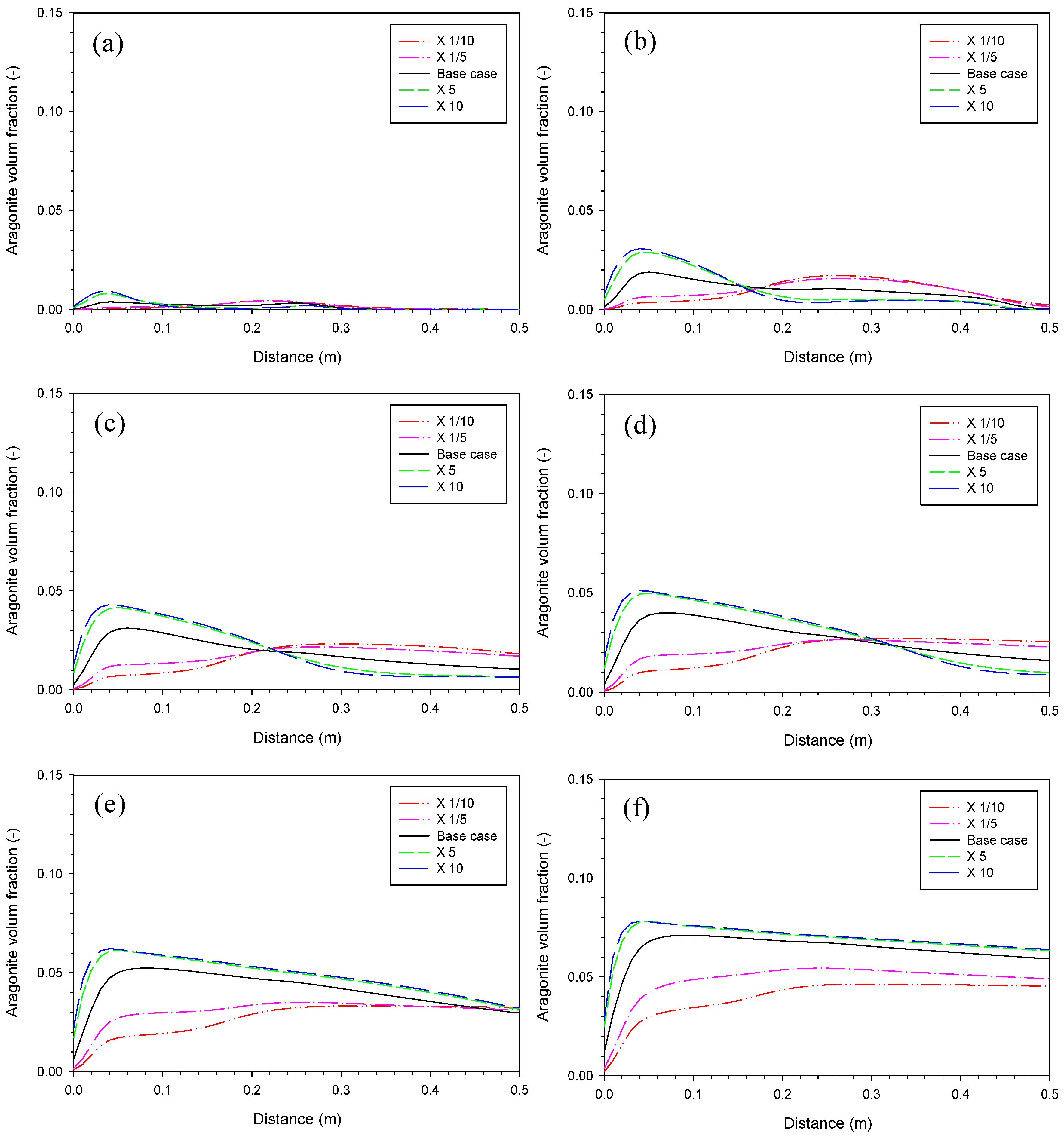
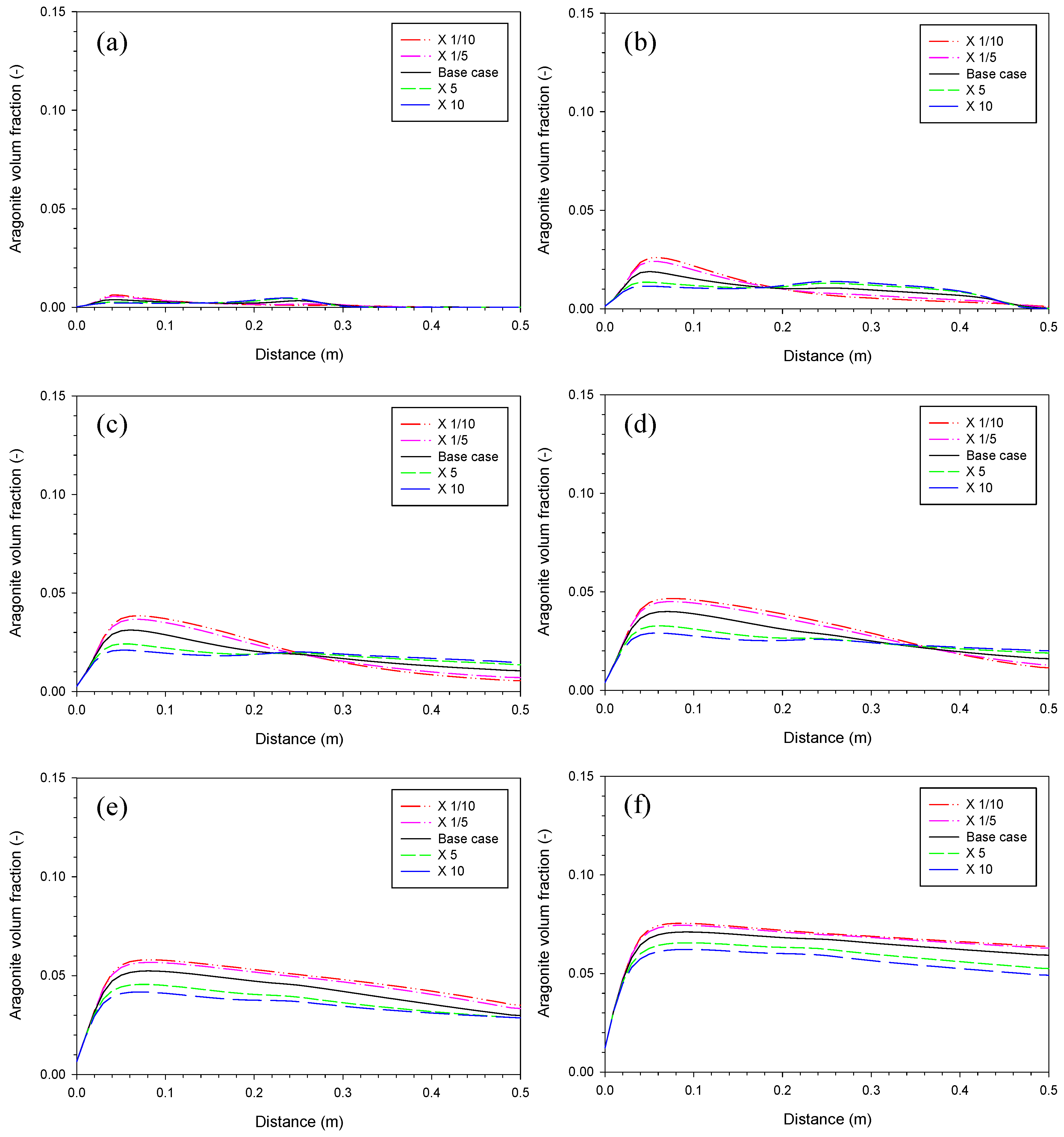
3.2. Aragonite Precipitation Rate

The range of the fitted CaCO₃(s)(aragonite) precipitation rate between different columns was within 1 order of magnitude [16]. However, the range for sensitivity analyses was selected to be over 2 orders of magnitude because the rate constant for CaCO₃(s) reported in the literature [32] was about 1−2 orders of magnitude lower than the range of the fitted aragonite precipitation rate.

Figure 3 and Figure 4 show the effect of aragonite precipitation rate on the TCE profiles and aragonite volume fraction at different times, respectively. The effect of the aragonite precipitation rate was prominent over the range at which that the sensitivity analyses were conducted, as seen in the differences in the curvature of the TCE profiles that evolved over time (Figure 3). TCE was degraded much faster at a slower aragonite precipitation rate because of a slower increase in aragonite accumulation and thus a slower decrease in reactivity of the iron.

Aragonite precipitated further into the column at a slower precipitation rate, while aragonite precipitated closer to the influent end at a faster precipitation rate (Figure 4). However, eventually more aragonite was accumulated throughout the column at a faster aragonite precipitation rate (Figure 4e,f). Accumulation of mineral was dependent not only on the absolute value but also on the relative precipitation rate among other mineral phases. Therefore, at a slower aragonite precipitation rate, there was greater accumulation of Fe₂(OH)₂CO₃ near the influent end (not shown). Because the molar volume of Fe₂(OH)₂CO₃ is greater than that of aragonite, more porosity loss occurred in that region.

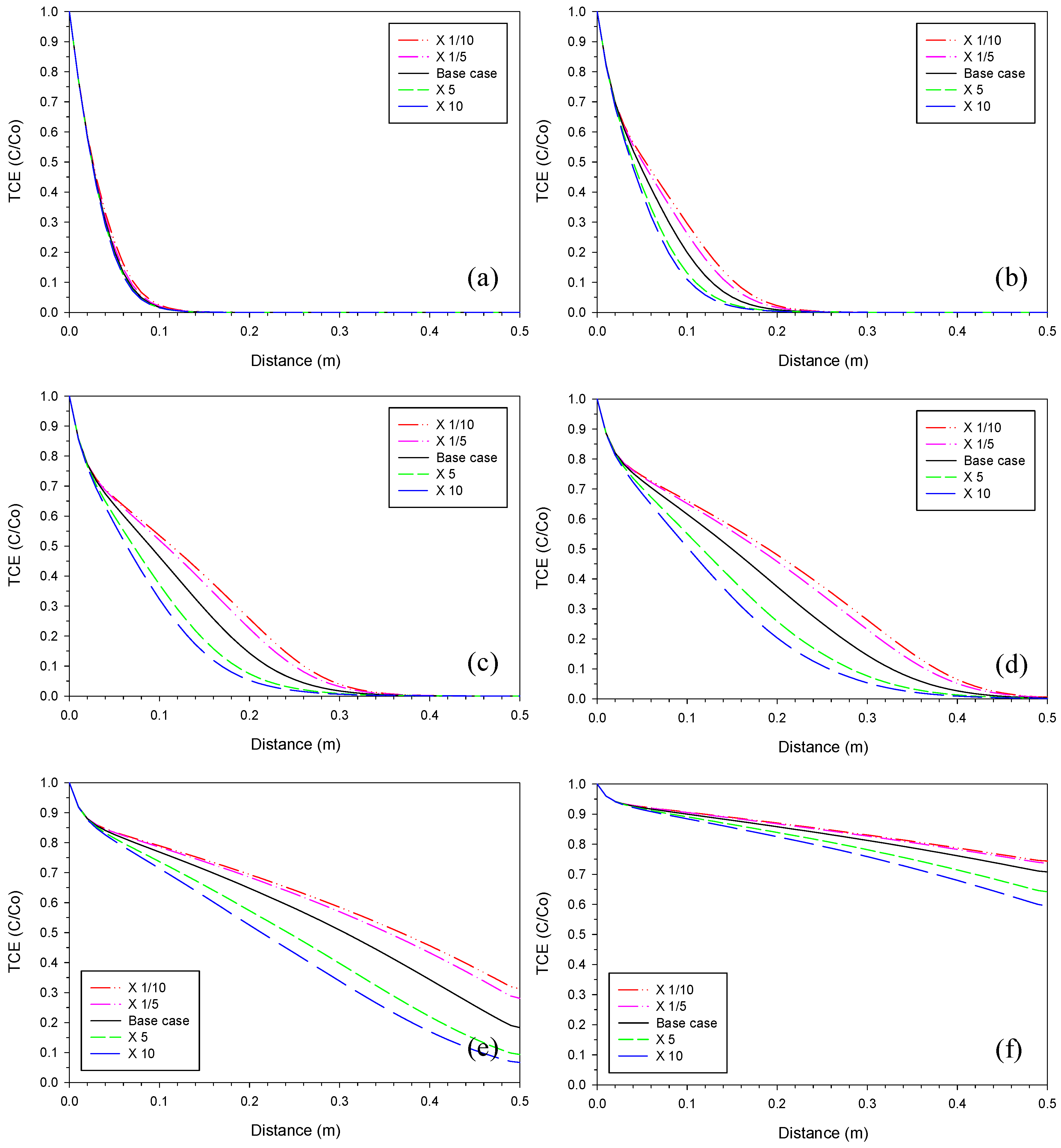
3.3. Fe₂(OH)₂CO₃ Precipitation Rate

The range for sensitivity analyses of Fe₂(OH)₂CO₃ precipitation rate was also selected to be over 2 orders of magnitude, based on the range of the fitted Fe₂(OH)₂CO₃ precipitation rate between different columns [16]. Generally, the effect of the Fe₂(OH)₂CO₃ precipitation rate was similar to that of aragonite, but in the opposite direction and to a lesser extent (Figure 5 and Figure 6). That is, at a slower Fe₂(OH)₂CO₃ precipitation rate, greater reactivity loss occurred because of more precipitation of aragonite, resulting in further migration of the TCE profiles (Figure 5). Because the Fe₂(OH)₂CO₃ precipitation rate indirectly affects the aragonite precipitation rate through a difference in relative precipitation rate, the extent to which Fe₂(OH)₂CO₃ precipitation rate affects the TCE profiles was much less than that of aragonite (Figure 3 and Figure 5).

For the accumulation of aragonite, at a slower Fe₂(OH)₂CO₃ precipitation rate, more aragonite was accumulated near the influent end of the column (Figure 6). Similar to the case of aragonite precipitation, eventually more aragonite was accumulated throughout the column at a slower Fe₂(OH)₂CO₃ precipitation rate (Figure 6e,f).

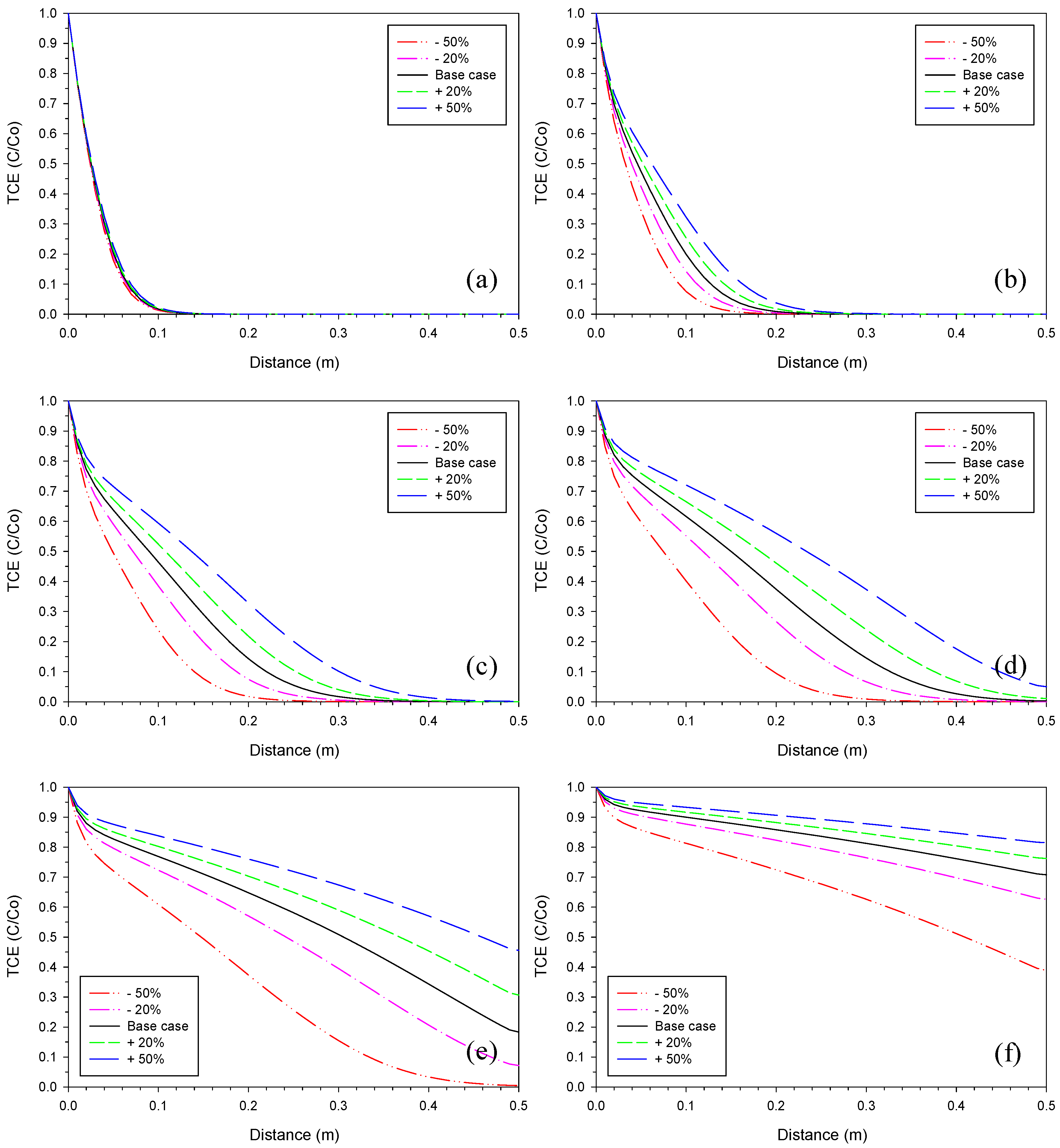
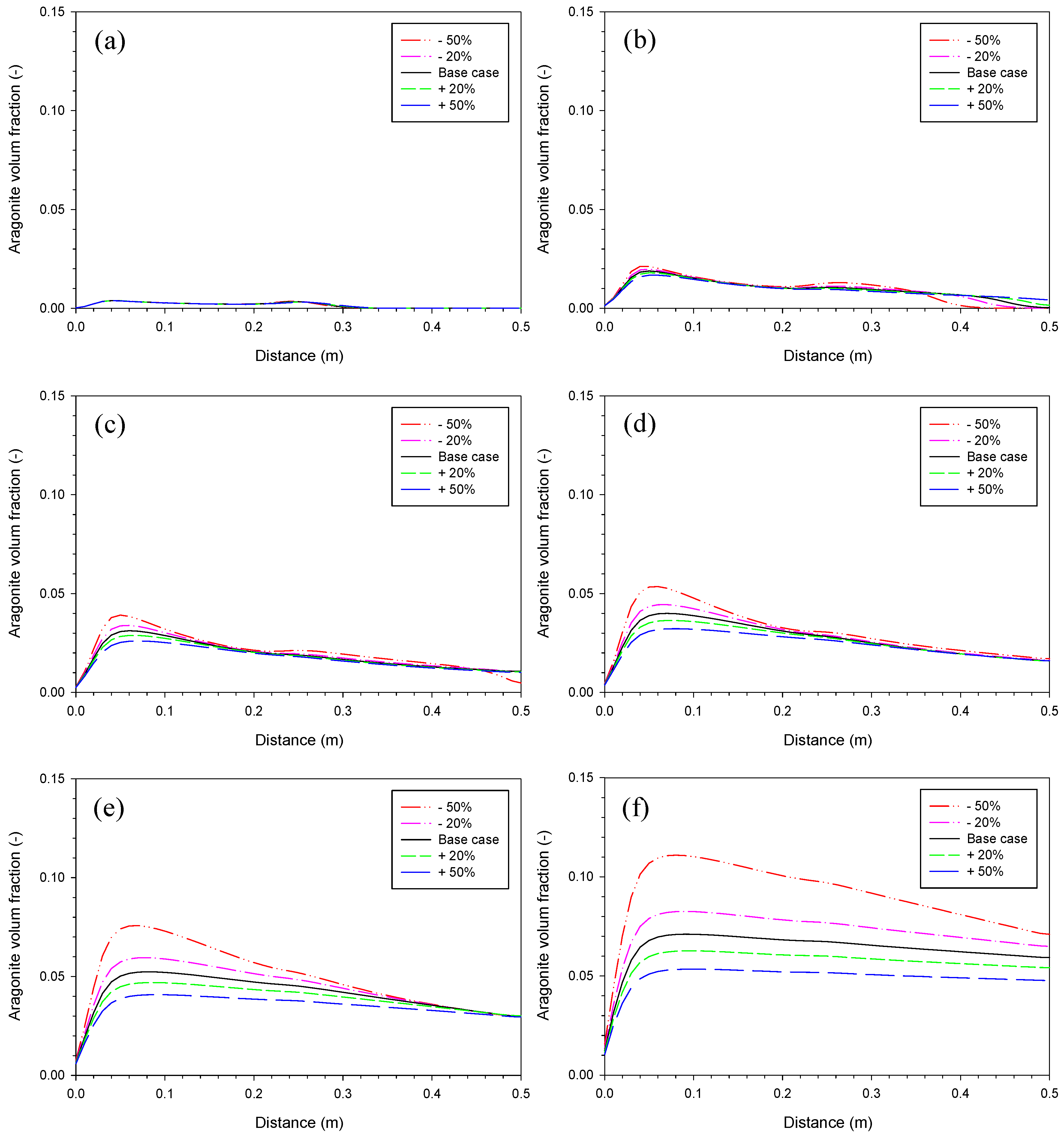
3.4. Proportionality Constant for Aragonite

The selected range for sensitivity analysis of a₁ (proportionality constant for aragonite) was +/−20%, +/−50%, which covers the maximum range of the fitted constant between different columns [16]. The proportionality constant for each mineral phase affects the extent to which the reactivity is decreased due to the accumulation of that mineral. Therefore, at a higher value of ${\mathsf{\alpha }}_1$, more migration of the TCE profiles occurred, as seen in Figure 7. In contrast, aragonite was accumulated more at a lower value of ${\mathsf{\alpha }}_1$, because a slower decrease in reactivity provided more potential for aragonite to accumulate in the same period of time (Figure 8).

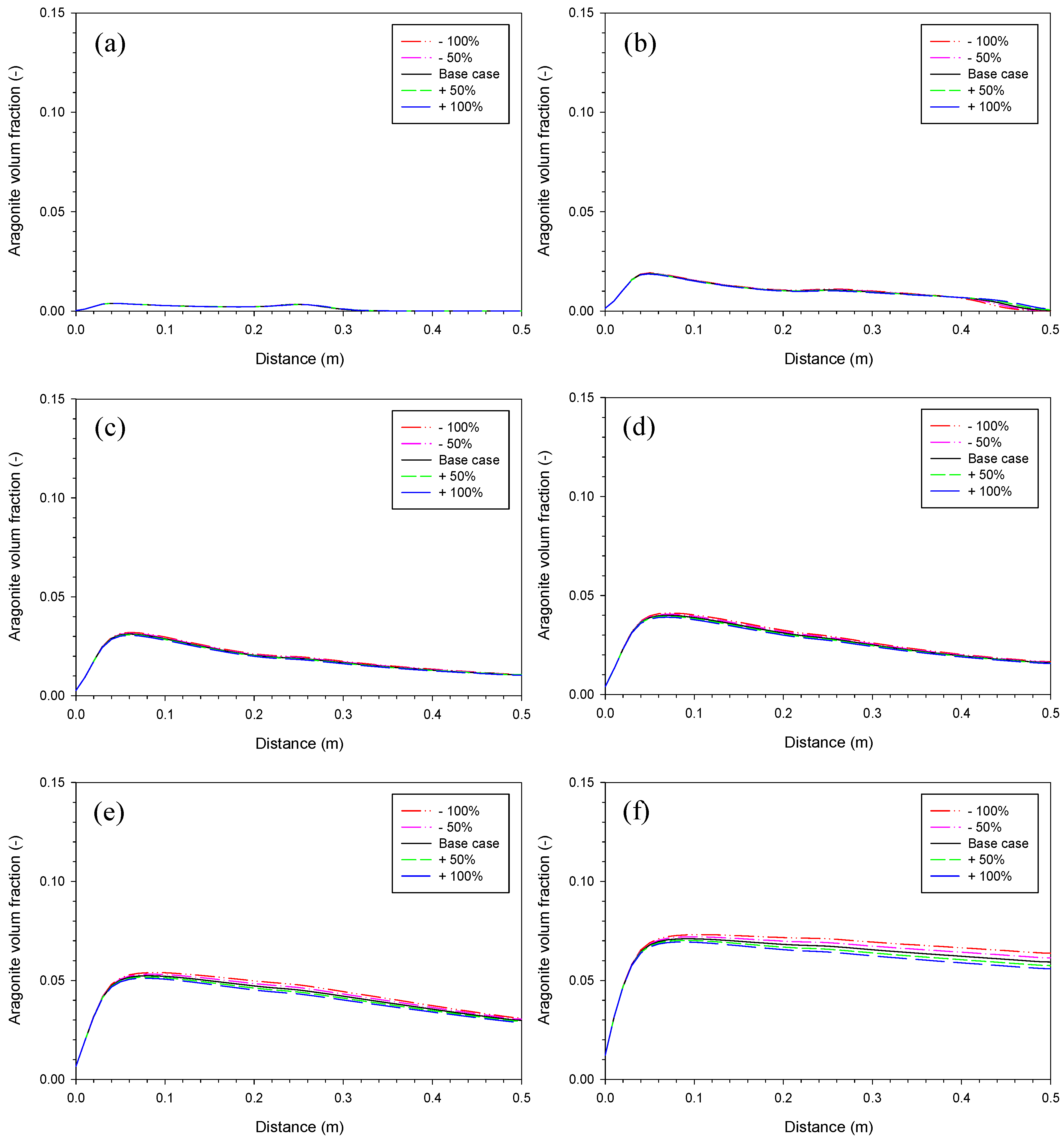
3.5. Proportionality Constant for Fe₂(OH)₂CO₃

Because the absolute value of the fitted ${\mathsf{\alpha }}_2$ (proportionality constant for Fe₂(OH)₂CO₃) was low (0.0–5.0 for all columns; [16]), the range of +/−100% for sensitivity analysis of ${\mathsf{\alpha }}_2$ does not necessarily mean a wide range of the parameter. Figure 9 and Figure 10 show the effect of ${\mathsf{\alpha }}_2$ on the TCE profiles and aragonite volume fraction at different times, respectively. As expected with the low value of ${\mathsf{\alpha }}_2$, the effect of this parameter was not significant. At a higher value of ${\mathsf{\alpha }}_2$, slightly more migration of the TCE profiles occurred over time (Figure 9). In contrast to the case of ${\mathsf{\alpha }}_1$, this parameter is applied to the accumulated volume fraction of Fe₂(OH)₂CO₃ instead of that of aragonite. Because the relative precipitation rates for each mineral do not change, the shape and pattern of aragonite accumulation was similar to the case of ${\mathsf{\alpha }}_1$. There was greater aragonite accumulation over time at a lower value of ${\mathsf{\alpha }}_2$, but the difference was not significant, as expected by the low value of ${\mathsf{\alpha }}_2$ (Figure 10).

4. Conclusions

To reliably predict long-term performance of a remediation system, it is necessary to constrain the parameters of a numerical model with validation of real data. Sensitivity analysis demonstrates how well a particular parameter is constrained and thus provides a basis for evaluation of geochemical profile changes over time. This study conducted sensitivity analyses for model parameters, which were shown to be important and also have some ranges to fit laboratory column data. Based on the previous modeling study, iron corrosion rate, aragonite and Fe₂(OH)₂CO₃ precipitation rates, and proportionality constants for each mineral were evaluated.

The iron corrosion rate affected TCE degradation and aragonite accumulation in proportion to the values of the rate. Secondary mineral precipitation rates were considered to be the most important parameters for predictive purposes. Interestingly, aragonite and Fe₂(OH)₂CO₃ precipitation rates affected each other in opposite ways, indicating that not only absolute precipitation rate for each mineral but also relative precipitation rates among different minerals are important for system performance. With higher values for the proportionality constants, the reactivity of iron for the treatment of TCE declined faster over time; however, it ended up with less accumulation of secondary minerals. This study implies that the reactivity and permeability of iron PRBs are not affected in the same direction.

Model parameters are often calibrated rather than directly measured because it is not possible to collect all necessary information with existing data. In this case, the parameters have some uncertainties, and thus model prediction should be interpreted with great care. The merit of model prediction is that it gives us implications with regard to future performance rather than precise particular numbers for certain scenarios. This study provides implications for long-term performance of granular iron PRBs which are affected by secondary mineral precipitation. It shows that the model can be a useful design tool if it is constrained with real data that are carefully generated by a laboratory test.

References

1. O’Hannesin, S.F.; Gillham, R.W. Long-term performance of an in-situ “iron wall” for remediation of VOCs. Ground Water 1998, 36, 164–170. [Google Scholar] [CrossRef]
2. Blowes, D.W.; Ptacek, C.J.; Benner, S.G.; McRae, C.W.T.; Puls, R.W. Treatment of dissolved metals and nutrients using permeable reactive barriers. J. Contam. Hydrol. 2000, 45, 123–137. [Google Scholar] [CrossRef]
3. Wilkin, R.T.; Acree, S.D.; Ross, R.R.; Beak, D.G.; Lee, T.R. Performance of a zerovalent iron reactive barrier for the treatment of arsenic in groundwater: Part 1. Hydrogeochemical studies. J. Contam. Hydrol. 2009, 106, 1–14. [Google Scholar] [CrossRef] [PubMed]
4. Obiri-Nyarko, F.; Grajales-Mesa, S.J.; Malina, G. An overview of permeable reactive barriers for in situ sustainable groundwater remediation. Chemosphere 2014, 111, 243–259. [Google Scholar] [CrossRef]
5. Li, J.; Dou, X.; Qin, H.; Sun, Y.; Yin, D.; Guan, X. Characterization methods of zerovalent iron for water treatment and remediation. Water Res. 2018, 148, 70–85. [Google Scholar] [CrossRef]
6. Phillips, D.H.; Van Nooten, T.; Bastiaens, L.; Russell, M.I.; Dickson, K.; Plant, S.; Ahad, J.M.E.; Newton, T.; Elliot, T.; Kalin, R.M. Ten year performance evaluation of a field-scale zero-valent iron permeable reactive barrier installed to remediate trichloroethene contaminated groundwater. Environ. Sci. Technol. 2010, 44, 3861–3869. [Google Scholar] [CrossRef]
7. Dong, J.; Ding, L.; Wen, C.; Hong, M.; Zhao, Y. Effects of geochemical constituents on the zero-valent iron reductive removal of nitrobenzene in groundwater. Water Environ. J. 2013, 27, 20–28. [Google Scholar] [CrossRef]
8. Jeen, S.-W.; Yang, Y.; Gui, L.; Gillham, R.W. Treatment of trichloroethene and hexavalent chromium by granular iron in the presence of dissolved CaCO3. J. Contam. Hydrol. 2013, 144, 108–121. [Google Scholar] [CrossRef]
9. Guan, X.; Sun, Y.; Qin, H.; Li, J.; Lo, I.M.C.; He, D.; Dong, H. The limitations of applying zero-valent iron technology in contaminants sequestration and the corresponding countermeasures: the development in zero-valent iron technology in the last two decades (1994–2014). Water Res. 2015, 75, 224–248. [Google Scholar] [CrossRef]
10. Ansaf, K.V.K.; Ambika, S.; Nambi, I.M. Performance enhancement of zero valent iron based systems using depassivators: Optimization and kinetic mechanisms. Water Res. 2016, 102, 436–444. [Google Scholar] [CrossRef]
11. Tang, F.; Xin, J.; Zheng, T.; Zheng, X.; Yang, X. Individual and combined effects of humic acid, bicarbonate and calcium on TCE removal kinetics, aging behavior and electron efficiency of mZVI particles. Chem. Eng. J. 2017, 324, 324–335. [Google Scholar] [CrossRef]
12. Flury, B.; Frommer, J.; Eggenberger, U.; Mäder, U.; Nachtegaal, M.; Kretzschmar, R. Assessment of long-term performance and chromate reduction mechanisms in a field scale permeable reactive barrier. Environ. Sci. Technol. 2009, 43, 6786–6792. [Google Scholar] [CrossRef] [PubMed]
13. Yabusaki, S.; Cantrell, K.; Sass, B.; Steefel, C. Multicomponent reactive transport in an in situ zero-valent iron cell. Environ. Sci. Technol. 2001, 35, 1493–1503. [Google Scholar] [CrossRef] [PubMed]
14. Li, L.; Benson, C.H. Evaluation of five strategies to limit the impact of fouling in permeable reactive barriers. J. Hazard. Mater. 2010, 181, 170–180. [Google Scholar] [CrossRef] [PubMed]
15. Weber, A.; Ruhl, A.S.; Amos, R.T. Investigating dominant processes in ZVI permeable reactive barriers using reactive transport modeling. J. Contam. Hydrol. 2013, 151, 68–82. [Google Scholar] [CrossRef] [PubMed]
16. Jeen, S.-W.; Mayer, K.U.; Gillham, R.W.; Blowes, D.W. Reactive transport modeling of trichloroethene treatment with declining reactivity of iron. Environ. Sci. Technol. 2007, 41, 1432–1438. [Google Scholar] [CrossRef]
17. Jeen, S.-W.; Amos, R.T.; Blowes, D.W. Modeling gas formation and mineral precipitation in a granular iron column. Environ. Sci. Technol. 2012, 46, 6742–6749. [Google Scholar] [CrossRef]
18. Jeong, H.Y.; Jeen, S.-W. Geochemical interactions of mine seepage water with an aquifer: Laboratory tests and reactive transport modeling. Environ. Earth Sci. 2016, 2016. 75, 1333. [Google Scholar] [CrossRef]
19. Jeen, S.-W. Reactive transport modeling for mobilization of arsenic in a sediment downgradient from an iron permeable reactive barrier. Water 2017, 9, 890. [Google Scholar] [CrossRef]
20. Jeen, S.-W.; Gillham, R.W.; Przepiora, A. Predictions of long-term performance of granular iron permeable reactive barriers: Field-scale evaluation. J. Contam. Hydrol. 2011, 123, 50–64. [Google Scholar] [CrossRef]
21. Mayer, K.U.; Frind, E.O.; Blowes, D.W. Multicomponent reactive transport modeling in variably saturated porous media using a generalized formulation for kinetically controlled reactions. Water Resour Res. 2002, 38, 1174. [Google Scholar] [CrossRef]
22. Steefel, C.I.; Lasaga, A.C. A coupled model for transport of multiple chemical species and kinetic precipitation/dissolution reactions with application to reactive flow in single phase hydrothermal systems. Am. J. Sci. 1994, 294, 529–592. [Google Scholar] [CrossRef]
23. Lichtner, P.C. Continuum Formulation of Multicomponent-Multiphase Reactive Transport. In Reactive Transport in Porous Media. Review in Mineralogy, vol. 34; Lichtner, P.C., Steefel, C.I., Oelkers, E.H., Eds.; Mineralogical Society of America: Washington, DC, USA, 1996; pp. 1–81. [Google Scholar]
24. Lichtner, P.C. Continuum model for simultaneous chemical reactions and mass transport in hydrothermal systems. Geochim. Cosmochim. Ac. 1985, 49, 779–800. [Google Scholar] [CrossRef]
25. Sevougian, S.D.; Schechter, R.S.; Lake, W. Effect of partial local equilibrium on the propagation of precipitation/dissolution waves. Ind. Eng. Chem. Res. 1993, 32, 2281–2304. [Google Scholar] [CrossRef]
26. Zhang, Y.; Gillham, R.W. Effects of gas generation and precipitates on performance of Fe0 RRBs. Ground Water 2005, 43, 113–121. [Google Scholar] [CrossRef] [PubMed]
27. Lu, Q.; Jeen, S.-W.; Gui, L.; Gillham, R.W. Nitrate reduction and its effects on trichloroethylene degradation by granular iron. Water Res. 2017, 112, 48–57. [Google Scholar] [CrossRef] [PubMed]
28. Jeen, S.-W.; Gillham, R.W.; Blowes, D.W. Effects of carbonate precipitates on long-term performance of granular iron for reductive dechlorination of TCE. Environ. Sci. Technol. 2006, 40, 6432–6437. [Google Scholar] [CrossRef] [PubMed]
29. Allison, J.D.; Brown, D.S.; Novo-Gradac, K.J. MINTEQA2/PRODEFA2, A Geochemical Assessment Model for Environmental Systems: Version 3.0 User’s Manual; EPA-600/3-91-021; U.S. Environmental Protection Agency: Athens, GA, USA, 1991.
30. Ball, J.W.; Nordstrom, D.K. User’s Manual for WATEQ4F, with Revised Thermodynamic Database and Test Cases for Calculating Speciation of Major, Trace, and Redox Elements in Natural Waters; Open-File Report 91-183; U.S. Geological Survey: Menlo Park, CA, USA, 1991.
31. Freeze, R.A.; Cherry, J.A. Groundwater; Prentice-Hall: Englewood Cliffs, NJ, USA, 1979. [Google Scholar]
32. Mayer, K.U.; Blowes, D.W.; Frind, E.O. Reactive transport modeling of an in situ reactive barrier for the treatment of hexavalent chromium and trichloroethylene in groundwater. Water Resour. Res. 2001, 37, 3091–3103. [Google Scholar] [CrossRef] [Green Version]
Figure 1. Sensitivity analysis of iron corrosion rate. TCE profiles on (a) Day 4, (b) Day 25, (c) Day 54, (d) Day 87, (e) Day 164, and (f) Day 410 with value of the base case, +/−20% and +/−50%.
Water 10 01878 g001
Figure 2. Sensitivity analysis of iron corrosion rate. Aragonite volume fraction on (a) Day 4, (b) Day 25, (c) Day 54, (d) Day 87, (e) Day 164, and (f) Day 410 with value of the base case, +/−20% and +/−50%.
Water 10 01878 g002
Figure 3. Sensitivity analysis of aragonite precipitation rate. TCE profiles on (a) Day 4, (b) Day 25, (c) Day 54, (d) Day 87, (e) Day 164, and (f) Day 410 with value of the base case, ×1/10, ×1/5, ×5, and ×10.
Water 10 01878 g003
Figure 4. Sensitivity analysis of aragonite precipitation rate. Aragonite volume fraction on (a) Day 4, (b) Day 25, (c) Day 54, (d) Day 87, (e) Day 164, and (f) Day 410 with value of the base case, ×1/10, ×1/5, ×5, and ×10.
Water 10 01878 g004
Figure 5. Sensitivity analysis of Fe2(OH)2CO3(s) precipitation rate. TCE profiles on (a) Day 4, (b) Day 25, (c) Day 54, (d) Day 87, (e) Day 164, and (f) Day 410 with value of the base case, ×1/10, ×1/5, ×5, and ×10.
Water 10 01878 g005
Figure 6. Sensitivity analysis of Fe2(OH)2CO3(s) precipitation rate. Aragonite volume fraction on (a) Day 4, (b) Day 25, (c) Day 54, (d) Day 87, (e) Day 164, and (f) Day 410 with value of the base case, ×1/10, ×1/5, ×5, and ×10.
Water 10 01878 g006
Figure 7. Sensitivity analysis of α 1 (proportionality constant for aragonite). TCE profiles on (a) Day 4, (b) Day 25, (c) Day 54, (d) Day 87, (e) Day 164, and (f) Day 410 with value of the base case, +/−20% and +/−50%.
Water 10 01878 g007
Figure 8. Sensitivity analysis of α 1 (proportionality constant for aragonite). Aragonite volume fraction on (a) Day 4, (b) Day 25, (c) Day 54, (d) Day 87, (e) Day 164, and (f) Day 410 with value of the base case, +/−20% and +/−50%.
Water 10 01878 g008
Figure 9. Sensitivity analysis of α 2 (proportionality constant for Fe2(OH)2CO3(s)). TCE profiles on (a) Day 4, (b) Day 25, (c) Day 54, (d) Day 87, (e) Day 164, and (f) Day 410 with value of the base case, +/−50% and +/−100%.
Water 10 01878 g009
Figure 10. Sensitivity analysis of α 2 (proportionality constant for Fe2(OH)2CO3(s)). Aragonite volume fraction on (a) Day 4, (b) Day 25, (c) Day 54, (d) Day 87, (e) Day 164, and (f) Day 410 with value of the base case, +/−50% and +/−100%.
Water 10 01878 g010