The Numerical Modeling of Coupled Motions of a Moored Floating Body in Waves

Abstract

Nonlinear interactions between water waves and a moored floating body are investigated using the virtual boundary force (VBF) method. The paper first introduces an in-house three-dimensional viscous incompressible flow model (NEWTANK), which is used to simulate wave-floating structure interaction by using the VBF method. Then the coupling procedure between the mooring line model and the floater model is described. Some validation cases of the developed model, including the motions of a free-floating box in two different water waves, are presented. The present numerical results will be compared with the available experimental data and other numerical results from the published literature. After that, the validity of the mooring line in the numerical model is simulated by simulating the motions of a floating box in still water. Finally, the verified model is applied to analyze the wave-induced motions of a catenary moored floating structure, investigating the motion responses and mooring forces responses. The numerical results agree well with the experimental measurements on the whole. This indicates that the present numerical model can correctly capture the main features of the wave-moored floating structure interaction.

1. Introduction

To limit the motions of a floating object (i.e., buoy, pontoon, floating breakwater, etc.) in an ocean environment, mooring lines are often used. Traditionally, the analysis of the motion of the moored floating body is generally conducted for regular waves using potential flow theory. Williams and Abul-Azm [1] investigated the wave reflection properties of a floating breakwater using the boundary integral equation method. Sannasiraj et al. [2] built a two-dimensional finite element model to investigate the behavior of floating pontoon breakwaters in beam waves. Williams et al. [3] studied the hydrodynamic properties of a pair of pontoon-type floating breakwaters by the boundary integral equation method using an appropriate Green’s function. By integration of the second-order fluid pressure, Chen et al. [4] analyzed the generalized first- and second-order fluid forces of a moored floating body used in the nonlinear hydroelastic analysis. Based on the high-order boundary element method, Wen [5] investigated the interaction between regular waves and two floating bodies in the frequency domain. Ku and Cha [6] analyzed the behavior of the coupled mooring system and floating bodies using non-linear finite element method.

However, although potential flow theory has been successfully used to simulate many interaction problems between non-breaking waves and a floating body, it is not applicable when the flow around the body is rotational, which can occur when waves break or the KC >> 1 (i.e., the body size is much smaller than the fluid trajectory under a wave). In addition, the potential flow cannot be applied to simulate the wave overtopping cases [7,8]. Theoretically, potential flow is not suitable for dealing with all the problems related to viscous effects, which limits its application in coastal engineering.

In recent years, there is an increasing number of studies on modeling fluid interaction with structures or wave interaction with moored floating bodies using viscous models. For example, Xue et al. [9,10] developed a three-dimensional numerical wave tank model and the corresponding physical model [11] for studying liquid sloshing dynamics and related problems. In their model, a coupled virtual boundary force with the volume of the fluid method was proposed to simulate wave interaction with internal structures. Rahman et al. [12] developed a two-dimensional numerical model, which combines the VOF model and porous body model, to investigate the dynamic responses of a submerged breakwater moored by inclined tension legs under wave action. Peng et al. [13] studied the interactions between water waves and inclined-moored floating breakwater using a viscous flow model. Their studies only focused on the submerged floating structures in two-dimensional space. Loukogeorgaki and Angelides [14] built a three-dimensional model to investigate the dynamic response of a moored floating breakwater in frequency domain under the action of regular waves. Ji et al. [15,16,17] carried out a series of experimental research on a dual cylindrical pontoon-net floating breakwater. Their numerical research is still conducted on a two-dimensional model which cannot capture the three-dimensional characteristics of waves in wave-structure interactions.

The in-house three-dimensional viscous flow model (NEWTANK) which was built by Liu and Lin [18] is mainly applied to the liquid sloshing and water wave problems in the previous studies [19,20,21]. In this paper, the in-house model (NEWTANK) will be further developed to investigate the wave interaction with a moored floating structure. A mooring line model based on the catenary method is built in the improved model. In this model, the virtual boundary force (VBF) method [19,21] is used to simulate the fluid-structure interaction. The coupling procedure between the mooring line model and the floater model is described in Section 2.

The paper is organized as follows: Section 2 describes the details of the present numerical model. In Section 3, some validation cases of the improved model are present at first. Then the verified model is applied to analyze the wave-induced motions of a moored floating structure. Finally, some important conclusions are drawn in Section 4.

2. Numerical Methods

2.1. Fluid Flow Governing Equations

In the framework of the NEWTANK model, the governing equations for unsteady incompressible flow are

$$\frac{\partial u_i}{\partial x_i}=0,$$

(1)

$$\frac{\partial u_i}{\partial t}+u_j\frac{\partial u_i}{\partial x_j}=-\frac{1}{\rho }\frac{\partial p}{\partial x_i}+(\nu +{\nu }_t){\nabla }^2{u}_i+g_i+f_{VBFi},$$

(2)

where $u_i$, i = 1, 2, 3, denotes the i-th component of the velocity vector, t is the time, $\rho$ is the density of the fluid, $p$ is the pressure, $g_i$ is the i-th component of the gravitational acceleration, $f_{VBFi}$ is the i-th component of the VBF which is zero everywhere except on the solid body surface. $v$ is the molecular kinematic viscosity and ${\nu }_t$ is the sub-grid-scale (SGS) eddy kinematic viscosity simulated by the LES turbulence model. ${\nu }_t$ is evaluated by the Smargorinsky–Lilly SGS model [22] as follows

$${\nu }_t=C_s^2{\Delta }^2\sqrt{2S_{ij}{S}_{ij}},$$

(3)

where $C_s=0.15$ (see reference [23]), $\Delta$ is the filter cutoff width, $S_{ij}=\frac{1}{2}\left(\frac{\partial u_i}{\partial x_j}+\frac{\partial u_j}{\partial x_i}\right)$ is the local rate of strain of the flow. In the three-dimensional computations with a grid of different length $\Delta x$, width $\Delta y$ and height $\Delta z$ the filter cutoff width is obtained by $\Delta =\sqrt[3]{\Delta x\Delta y\Delta z}$.

The governing Equations (1) and (2) are solved numerically by a two-step projection method. In the first step, the intermediate velocity is computed by explicit computing the convective and diffusion terms in the momentum equation. In the second step, the pressure is obtained by solving a Poisson equation and then applied to the velocity field to satisfy the divergence-free condition. Finally, the final divergence-free velocity is updated by simple algebraic operations.

In this model, a combination of the upwind scheme and the central difference scheme is adopted in the discretization of the convection term. A second-order central difference scheme is used for the diffusion term. The detailed numerical scheme about this model can be found in [18]. This model has a second-order spatial accuracy and first-order accuracy in time, which meets the needs of simulating wave-structure interactions [21]. The grid independence of this model is validated in the previous study [21].

A staggered fixed Cartesian grid system that covers the whole computational domain is used. The VBF method is used to simulate the interaction between the structure and fluid in this numerical model. The free surface motion is tracked by the volume of fluid (VOF) method with a second-order piecewise linear interface calculation (PLIC) method according to Reference [24].

2.2. Equations for Mooring Line Dynamics

Most mooring lines used in marine applications are very long and slender structures. Hence, the mooring line is always supposed to a homogeneous line in theoretical analysis. Here we analyze a moored floating body which is connected to the sea floor by a mooring line. Four different states of a mooring line—the totally relaxed (case a), catenary state (case b), partially extended (case c) and totally extended (case d)—are illustrated in Figure 1. The anchor is located at point A, and the position of the mooring point is B. The total length of the mooring line is L, and $l$ denotes the free hanging length of the mooring line. The horizontal distance between point A and point B is S. The net weight per unit length of the mooring line is ${\rho }_{m}g$.

For state a, the mooring line is vertically hanging under the floating body. It is the simplest state for the force analysis. The mooring force acted on the floating body equal to the weight of the hanging section of the mooring line, i.e.,

$$T={\rho }_{m}gl,$$

(4)

For the state b, the mooring line is partially lifted, and the section near the anchor keeps the horizontal state. This state is usually called catenary state. According to the force analysis, the mooring force exerted on the floating body can be calculated by the following equation.

$$L-S=\sqrt{h^2+2ah}-a\mathrm{arcosh}\frac{h+a}{a},$$

(5)

Newton’s iteration method is used to get the value of parameter a. Then we can get the horizontal mooring force $Q={\rho }_{m}ga$ and the vertical component of the mooring force $V={\rho }_{m}gl$. The total mooring force is

$$T=\sqrt{Q^2+V^2}={\rho }_{m}g\sqrt{a^2+l^2}={\rho }_{m}g(a+h),$$

(6)

For the state c, the mooring line is partially extended. The section at the anchor is no longer remain horizontal. The mooring force can be calculated by the following equation.

$$\frac{h^2-L^2}{2a}=1-\cosh \frac{S}{a},$$

(7)

Similarly, the value of a gets by Newton’s iteration method. Then the horizontal mooring force is $Q={\rho }_{m}ga$. The vertical mooring force is $V=Q\tan \alpha$ at the position of the anchor. The total mooring force acted on the floating body is

$$T=\sqrt{Q^2+{({\rho }_{m}gL+V)}^2},$$

(8)

For the state d, the mooring line is totally extended. e is the elastic coefficient of the mooring line. If the mooring line is extended $\Delta l$, the horizontal mooring force acted on the floating body is $Q=e\Delta l\cos \theta$, and the vertical mooring force is $V=e\Delta l\cos \theta +{\rho }_{m}gL$.

2.3. Equations for Floating Body Dynamics

By solving the fluid equations and mooring line equations, we can get the value of the wave force and mooring force acted on the floating body. Following Newton’s second law of motion, the motions of a moored floating body can be governed by the following equations.

$$\{\begin{array}{l}M\frac{dV}{dt}=Mg+F_m+{\displaystyle \underset{s}{\iint }PndS}\\ I\frac{d\Omega }{dt}=(r_m-R_0)\times F_m+{\displaystyle \underset{s}{\iint }(r_P-R_0)\times PndS}\end{array},$$

(9)

where M represents the mass of the floating body, I represents the moment of inertia of the floating body, $V$ is the linear velocity of the mass center, and $\Omega$ is the angular velocity of the mass center. The subscript $S$ denotes the surface of the object, and $n$ is the unit normal vector of the body surface. $R_0$ represents the position of the mass center of the object. $r_m$ is the position of the mooring force $F_m$ acted on the floating body, and $r_P$ is the position of the pressure working point.

2.4. Numerical Stability Criterion

There are two stability criteria that must be satisfied to ensure the stability of the scheme. One criterion is derived from the Courant–Friedrichs–Lewy (CFL) condition and is related to the convection process, and the other criterion is connected with the diffusion process:

$$\Delta t\le \min \left(\frac{Cr\times \Delta x}{u_{\max }},\frac{Cr\times \Delta y}{v_{\max }},\frac{Cr\times \Delta z}{w_{\max }},\frac{\Delta x^2}{6\nu },\frac{\Delta y^2}{6\nu },\frac{\Delta z^2}{6\nu }\right),$$

(10)

where $u_{\max }$, $v_{\max }$ and $w_{\max }$ are the maximum velocities in the x-direction, y-direction and z-direction, respectively. Throughout the following simulation, the value of the Courant number Cr is set to 0.3.

3. Numerical Validation and Discussion

In this section, two cases are simulated to validate the present numerical model in applications of water waves interaction with floating structures. The verified model is then applied to analyze the motions of a catenary moored floating structure in waves.

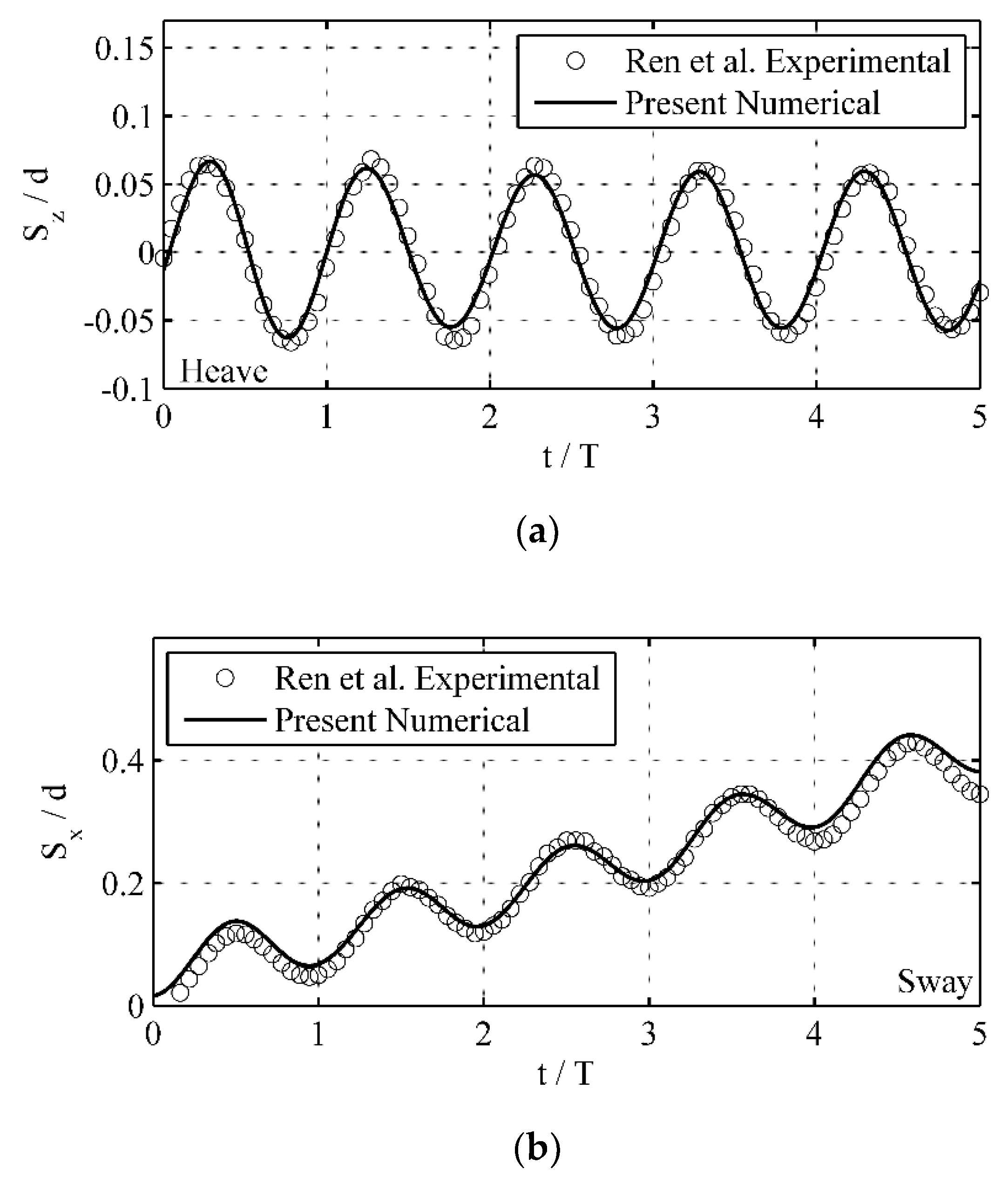
3.1. Motions of a Free-Floating Box in Waves

In this part, the present numerical model is used to investigate the motions of a free-floating box in regular water waves. Only some important parameters used in the simulation are listed here. For a more detailed setup of the experiment, the readers are referred to Reference [25]. A floating box with a width of $l_x=0.3 \mathrm{m}$ and a height of $l_z=0.2 \mathrm{m}$ is deployed in a flume that is $23 \mathrm{m}$ long and $0.44 \mathrm{m}$ wide (illustrated in Figure 2). The initial still water $h$ is $0.4 \mathrm{m}$. The average density of the floating box is $500 \mathrm{Kg}/{\mathrm{m}}^3$, thus the draught is $d=0.1 \mathrm{m}$.

The size of the numerical domain is $8.0 \mathrm{m}\times 0.56 \mathrm{m}$. A linear periodic wave train with different wave height ($H=0.04 \mathrm{m}$ and $H=0.1 \mathrm{m}$) and same wave period ($T=1.2 \mathrm{s}$) was sent from the left inflow boundary. The center of the floating box is 3.35 m away from the left inflow boundary. A sponge layer with a width of 2.0 m is set on the right-hand side of the computational domain to reduce the influence of the reflected waves.

The domain is discretized by 804 non-uniform grids in the x-direction with the finest grids ($\Delta x=0.005 \mathrm{m}$) being employed near the floating box, and 174 non-uniform grids are applied in the z-direction with the finest grids ($\Delta z=0.002 \mathrm{m}$) being arranged around the still water level. In order to satisfy the stability constraints, the computational time step is adjusted dynamically during the simulation.

The motions (including the heave $S_z$, sway $S_x$ and roll angle $\theta$) of the floating box are presented in Figure 3. Here the roll angle $\theta$ is positive when the floating box rolls in the clockwise direction. From Figure 3, the heave components and roll components are present simple harmonic oscillations, while the sway components include a drifting motion in the x-direction besides a simple harmonic oscillation. Although the wave height ($H=0.1 \mathrm{m}$) is larger than that of Figure 3 ($H=0.04 \mathrm{m}$), similar motion patterns can be observed from Figure 4. In addition, it is observed from Figure 3 and Figure 4 that the present numerical results agree well with the experimental measurements overall.

Figure 5 shows the trajectory of the free-floating box in a motion period under the regular wave. The agreement between the computed results and experiments’ measurements is still acceptable.

3.2. Motions of a Moored Floating Box in Still Water

In this section, a floating box in static water is initially set up with two asymmetric mooring lines in the catenary state, while the physical properties of two mooring lines (i.e., the length, the quality of the unit length, the cross-sectional area, etc.) are identical. The basic layout and coordinate system settings of the model are illustrated in Figure 6. In the initial state, the right mooring line is relatively more slack than the left one.

The computational domain size is 2.0 m × 0.7 m. The floating box is arranged at a deviation from the equilibrium position 5.0 cm. The two anchors are fixed on the bed and their horizontal distance from the equilibrium position is 0.35 m. The mooring lines are connected with the floating box as shown in Figure 6. The density of the floating box is $500 \mathrm{Kg}/{\mathrm{m}}^3$. The draught of the floating box is 0.1 m in the initial state. The still water depth h is 0.4 m. In order to restore the floating box to the equilibrium position more quickly, the kinematic viscosity coefficient of the fluid is set to $2.0\times {10}^{-4} {\mathrm{m}}^2/\mathrm{s}$. Each mooring line has a length of 0.35 m with a line density of 2.0 $\mathrm{N}/\mathrm{m}$. A non-uniform grid system of 300 × 64 is used in this simulation with the finest grid (0.005 m × 0.005 m) being employed near the floating box. In this simulation, the time step is adjusted dynamically according to the stable conditions.

The initially static floating box acted by the total horizontal mooring force is accelerated to the left. While the right mooring force gradually becomes stretched, the left mooring line gradually becomes slack. The total horizontal mooring force is gradually reduced to zero when the floating box reaches its maximum speed to the left. Under the action of inertia, the floating box continues to move to the left. The total horizontal mooring force turns to the right and gradually increases, which makes the speed of the floating box gradually decrease to zero. At this time, the floating box reaches the maximum displacement to the left. Then the floating box starts to move to the right under the action of the two mooring lines. Finally, the floating box achieves static equilibrium at the symmetry point under the periodic action of two mooring lines. Figure 7 shows the time sequences of the horizontal displacement of the mass center of the floating box, from which it can be observed that the floating box reaches its equilibrium point after 100 s and no longer swings.

Figure 8 shows the time sequences of the mooring force which includes the left-side horizontal mooring force, the right-side horizontal mooring force, and the total horizontal mooring force. The extremum of the total horizontal mooring force decreases gradually with time, and finally, the total horizontal mooring force returns to zero when the floating box returns to the equilibrium point. This is consistent with the theoretically expected results. There is a 180-degree phase difference in time between the total horizontal mooring force and the horizontal displacement of the floating box. For example, when the horizontal mooring force reaches the maximum value to the right, the floating box exactly reaches the maximum displacement to the left.

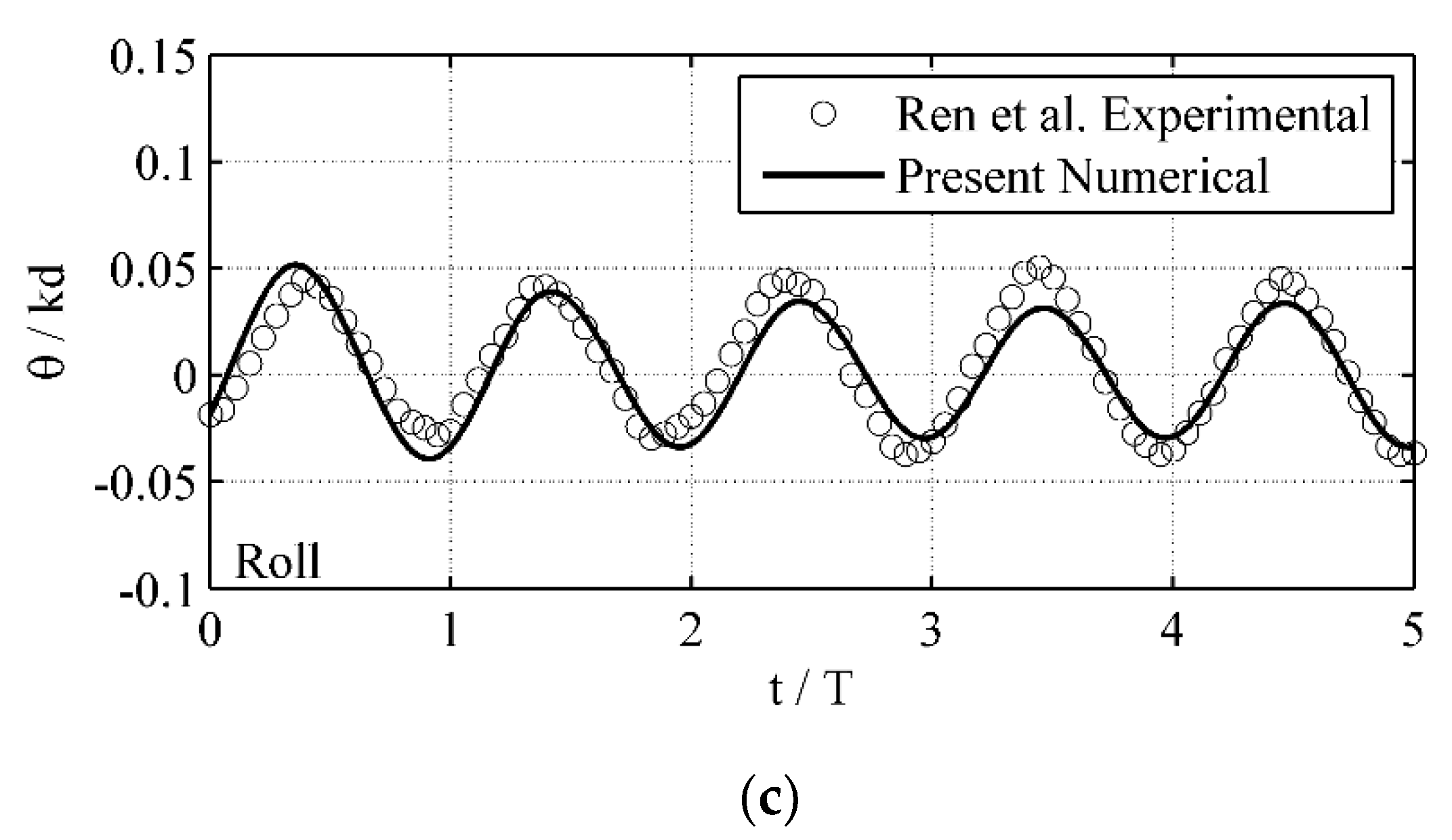
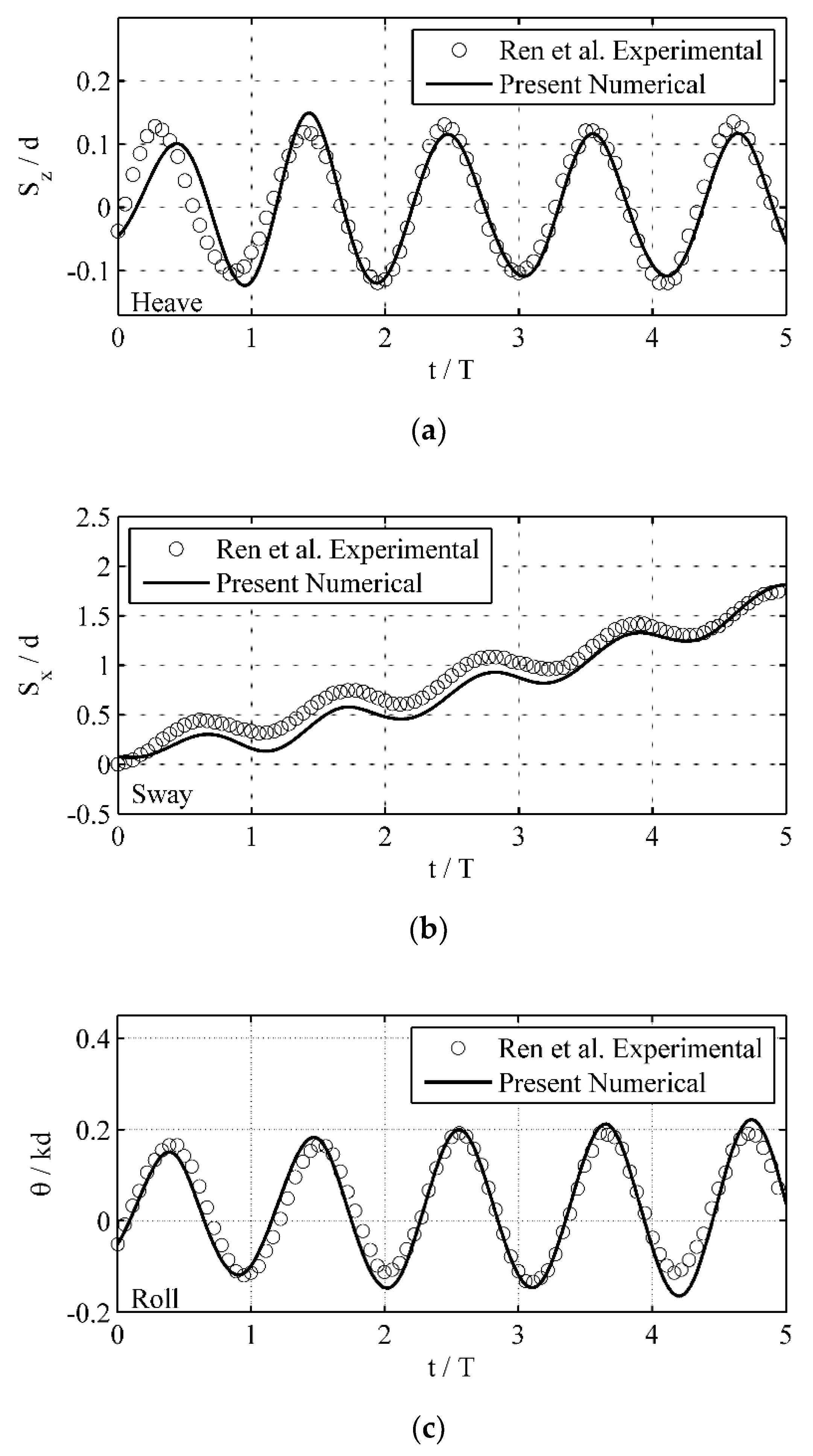
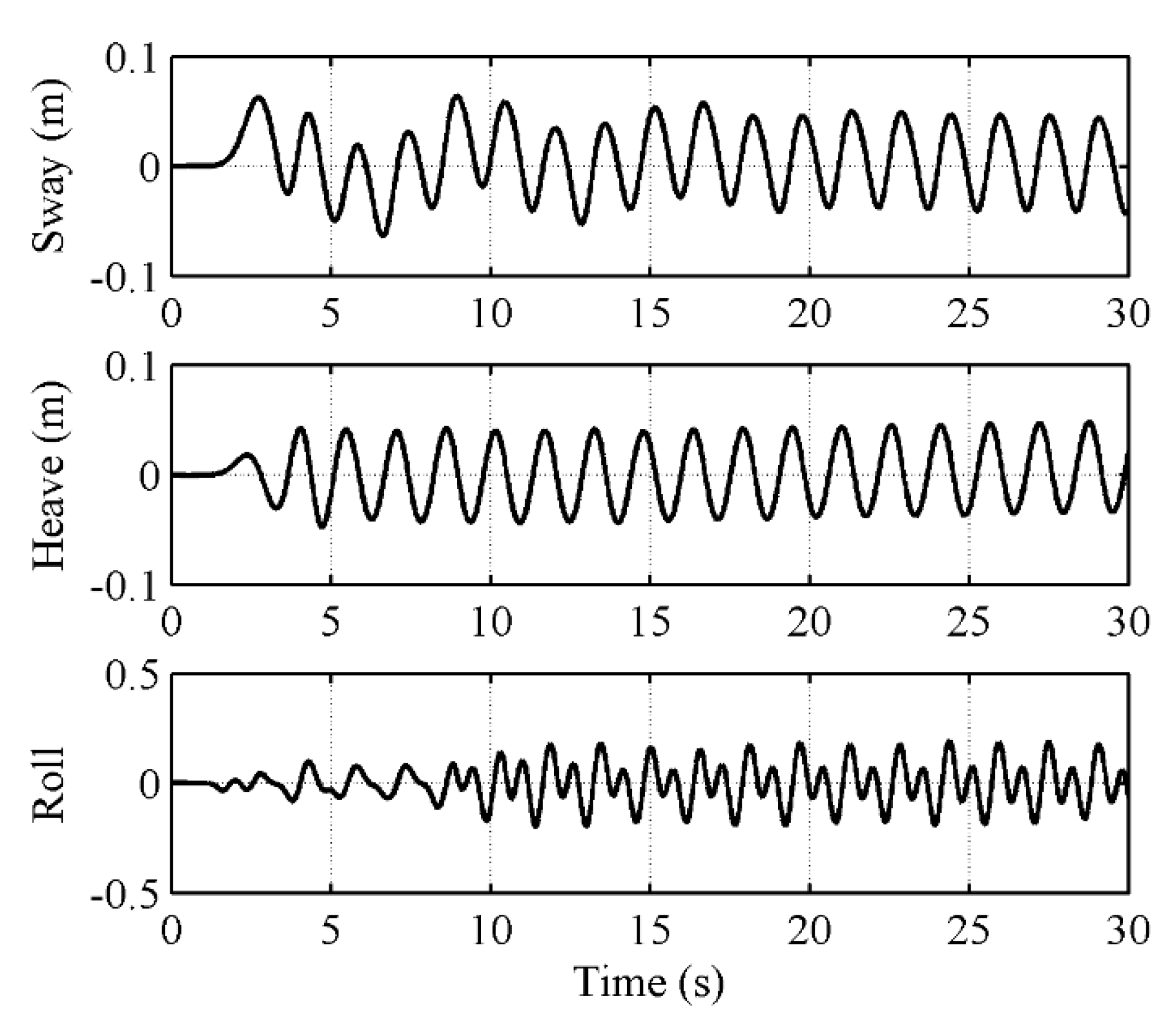
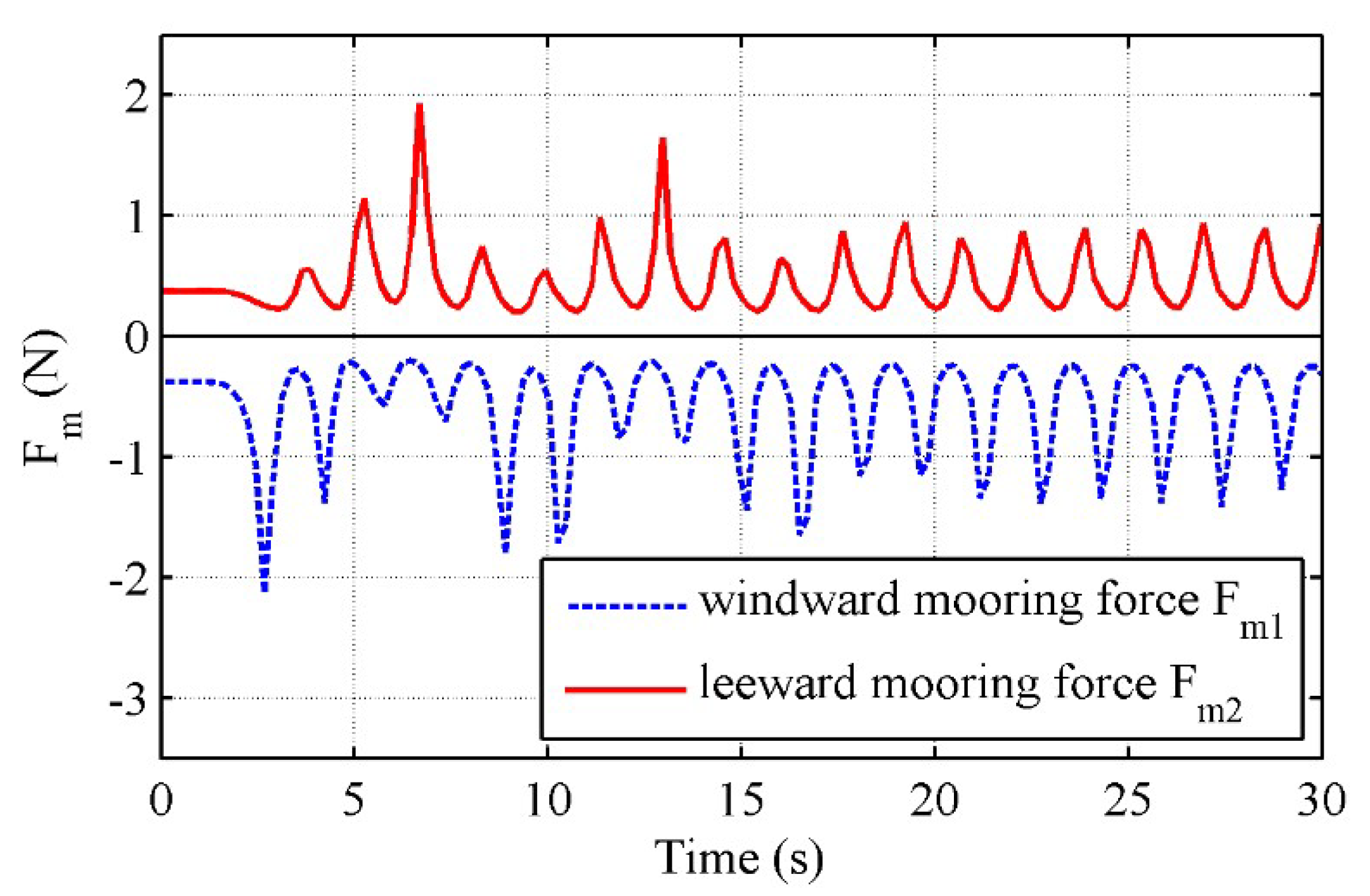
3.3. Motions of a Moored Floating Box in Waves

In this section, the validated numerical model is used to simulate the water wave interaction with a moored floating structure. A floating box that is 0.44 m long, 0.3 m wide, and 0.18 m high is deployed in a computational domain that measures 8 m × 0.45 m (illustrated in Figure 9). The initial still water h is 0.4 m. The center of the floating rectangle is 3.5 m away from the left inflow boundary (x = 0) of the computational domain. The draught d of the floating box is 0.135 m. The mass of the floating box is 17.82 Kg. In Figure 9, four mooring lines that are symmetrically arranged are used. Each mooring line has a length of 0.908 m with a line density of 36.165 $\mathrm{g}/\mathrm{m}$. The horizontally projected length of each mooring line is 0.798 m (illustrated in Figure 10), which is based on the flume experiments conducted by Mr. Hou in Dalian University of Technology and reported in Reference [26]. A regular water wave train of period T = 1.55 s and wave height H = 0.07 m is sent from the left inflow boundary.

In the computational domain, a non-uniform grids system is applied in the x-direction with the finest grids ($\Delta x=0.005 \mathrm{m}$) being arranged near the floating box. A uniform grids system ($\Delta y=0.005 \mathrm{m}$) is used in the y-direction. The time step is adjusted dynamically during the simulation to satisfy the criterion of the CFL number of 0.3. In order to reduce the influence of the reflected wave, a numerical sponge layer is arranged in the area near the right exit boundary. In order to achieve the best absorbing effect, the thickness of the sponge layer is set to 3.0 m (i.e., between 1 to 1.5 times the wavelength of the incident wave [27,28]).

Figure 11 shows the time sequences of the displacement of the floating box simulated by this model, which are sway, heave, and roll, respectively. It can be seen from Figure 11 that the heave components and sway components are present simple harmonic oscillations after the stable state is reached, while the roll components present a complex motion. This phenomenon is caused by the periodic action of the mooring lines on the floating box.

According to the second-order Stokes wave theory [29], the horizontal displacement of the water particle is

$$\begin{array}{l}\zeta =x_0-\frac{H}{2}\frac{\cosh k(h+z)}{\sinh kh}\sin (kx-\sigma t)\\ -\frac{k{H}^2}{8}\frac{1}{{\sinh }^{2}kh}\left[-\frac{1}{2}+\frac{3}{4}\frac{\cosh 2k(h+z)}{{\sinh }^{2}kh}\right]\sin 2(kx-\sigma t)\\ +\frac{\sigma k{H}^2}{8}\frac{\cosh 2k(h+z)}{{\sinh }^{2}kh}t,\end{array}$$

(11)

where $k$ represents wave number, $\sigma$ represents the angular frequency. When the incident wave parameters are put into the above formula, it is found that the horizontal displacement of the free surface water particle is 0.1 m in a wave period time. According to the numerical simulation results, the average of the amplitude of the floating box in a period is 0.08 m, which is less than the horizontal displacement of the water particle during a wave period. This indicates that the floating box does not follow the water body completely when it is affected by the mooring lines.

The response amplitude operators (RAO) of sway, heave, roll and mooring force are defined [2], respectively:

$\mathrm{RAO}\left(\mathrm{sway}\right)$ = sway amplitude/wave amplitude;

$\mathrm{RAO}\left(\mathrm{heave}\right)$ = heave amplitude/wave amplitude;

$\mathrm{RAO}\left(\mathrm{roll}\right)$ = roll amplitude/wave amplitude, the unit is °/cm;

$\mathrm{RAO}\left(\mathrm{mooring} \mathrm{force}\right)$ = mooring force amplitude/wave amplitude, the unit is $\mathrm{N}/\mathrm{cm}$.

Table 1. The comparison of measured and present numerical response amplitude operators (RAO) of the motion responses.

RAO	Experimental Data [26]	Present Result
RAO (sway)	1.17	1.23
RAO (heave)	1.14	1.19
RAO (roll): °/cm	1.42	2.09

shows a comparison of the experimental [25] and presents numerical RAO of the floating box motion. According to the data in Table 1, the simulation results of the RAO of three displacement components of the floating box are larger than the experimental measurements. In the physical experiment, the floating box movement is inevitably not affected by the edge wall of the flume, while the side wall in the numerical model has little influence on the motion of the floating box. For this reason, the moving amplitude of the floating box in the numerical model is larger than the physical experiment.

The time series of the windward and leeward mooring forces are shown in Figure 12. There is a 90-degree phase difference in time between the leeward mooring force and the windward mooring force. A comparison of the measured and present numerical RAO of the mooring forces is shown in

Table 2. The comparison of measured and present numerical response amplitude operators (RAO) of the mooring forces.

RAO	Experimental Data [26]	Present Result
RAO (Fm1): $\mathrm{N}/\mathrm{cm}$	0.392	0.390
RAO (Fm2): $\mathrm{N}/\mathrm{cm}$	0.392	0.245

. In the numerical results of the mooring force RAO, the windward value is greater than that of the leeward side, and the measured results are equal in the experiment. Based on the water wave theory, the floating box will bear the wave drift force at the windward side while the leeward side will not. Therefore, the numerical result of the mooring force RAO is more reasonable than that of the experimental measurement.

4. Conclusions

In this paper, a numerical wave tank coupled with a mooring line model is developed to investigate the water wave interaction with a surface-piercing moored floating structure. This numerical model is well validated by the simulation of a free-floating box moving in regular water waves and a moored floating box oscillating in still water. The model’s capability of dealing with a moored floating structure is proved and the accuracy of the numerical result is demonstrated.

The verified numerical model is then applied to investigate the wave-induced motions of a moored floating box. The motion responses in regular water waves are in agreement with the experimental measurements, indicating that the present model is a reliable tool in simulating the interaction between the water wave and moored floating structure in coastal and offshore engineering.

Although the current model can basically simulate the wave-induced motions of a moored floating structure, the model will need further improvements in the future, such as the interaction between the mooring line and fluid, multiple mooring line system, and the material properties of mooring lines.

References

1. Williams, A.; Abul-Azm, A. Dual pontoon floating breakwater. Ocean Eng. 1997, 24, 465–478. [Google Scholar] [CrossRef]
2. Sannasiraj, S.; Sundar, V.; Sundaravadivelu, R. Mooring forces and motion responses of pontoon-type floating breakwaters. Ocean Eng. 1998, 25, 27–48. [Google Scholar] [CrossRef]
3. Williams, A.; Lee, H.; Huang, Z. Floating pontoon breakwaters. Ocean Eng. 2000, 27, 221–240. [Google Scholar] [CrossRef]
4. Chen, X.; Wu, Y.; Cui, W.; Tang, X. Nonlinear hydroelastic analysis of a moored floating body. Ocean Eng. 2003, 30, 965–1003. [Google Scholar] [CrossRef]
5. Wen, J. Numerical and Experimental Study on the Interaction between Waves and Two Floating Bodies. Master’s Thesis, Dalian University of Technology, Dalian, China, 2012. [Google Scholar]
6. Ku, N.; Cha, J.-H. A Study on Moored Floating Body Using Non-Linear FEM Analysis. In Proceedings of the Twelfth ISOPE Pacific/Asia Offshore Mechanics Symposium, Gold Coast, Australia, 4–7 October 2016; International Society of Offshore and Polar Engineers: Mountain View, CA, USA, 2016. [Google Scholar]
7. Zhang, X.; Wolgamot, H.; Draper, S.; Zhao, W.; Cheng, L. The role of overtopping duration in greenwater loading. In Proceedings of the 33rd International Workshop on Water Waves and Floating Bodies, Guidel-Plages, France, 4–7 April 2018. [Google Scholar]
8. Zhang, X.; Draper, S.; Wolgamot, H.; Zhao, W.; Cheng, L. Numerical Investigation of Effects of Bow Flare Angle on Greenwater Overtopping a Fixed Offshore Vessel. In Proceedings of the ASME 2018 37th International Conference on Ocean, Offshore and Arctic Engineering, American Society of Mechanical Engineers, Madrid, Spain, 17–22 June 2018; p. V001T01A002. [Google Scholar]
9. Xue, M.; Lin, P.; Zheng, J.; Ma, Y.; Yuan, X.; Nguyen, V. Effects of perforated baffle on reducing sloshing in rectangular tank: Experimental and numerical study. China Ocean Eng. 2013, 27, 615–628. [Google Scholar] [CrossRef]
10. Xue, M.; Zheng, J.; Lin, P.; Xiao, Z. Violent transient sloshing-wave interaction with a baffle in a three-dimensional numerical tank. J. Ocean Univ. China 2017, 16, 661–673. [Google Scholar] [CrossRef]
11. Xue, M.; Zheng, J.; Lin, P.; Yuan, X. Experimental study on vertical baffles of different configurations in suppressing sloshing pressure. Ocean Eng. 2017, 136, 178–189. [Google Scholar] [CrossRef]
12. Rahman, M.A.; Mizutani, N.; Kawasaki, K. Numerical modeling of dynamic responses and mooring forces of submerged floating breakwater. Coast. Eng. 2006, 53, 799–815. [Google Scholar] [CrossRef]
13. Peng, W.; Lee, K.-H.; Shin, S.-H.; Mizutani, N. Numerical simulation of interactions between water waves and inclined-moored submerged floating breakwaters. Coast. Eng. 2013, 82, 76–87. [Google Scholar] [CrossRef]
14. Loukogeorgaki, E.; Angelides, D.C. Stiffness of mooring lines and performance of floating breakwater in three dimensions. Appl. Ocean Res. 2005, 27, 187–208. [Google Scholar] [CrossRef]
15. Ji, C.-Y.; Chen, X.; Cui, J.; Yuan, Z.-M.; Incecik, A. Experimental study of a new type of floating breakwater. Ocean Eng. 2015, 105, 295–303. [Google Scholar] [CrossRef] [Green Version]
16. Ji, C.-Y.; Guo, Y.-C.; Cui, J.; Yuan, Z.-M.; Ma, X.-J. 3D experimental study on a cylindrical floating breakwater system. Ocean Eng. 2016, 125, 38–50. [Google Scholar] [CrossRef]
17. Ji, C.; Cheng, Y.; Yang, K.; Oleg, G. Numerical and experimental investigation of hydrodynamic performance of a cylindrical dual pontoon-net floating breakwater. Coast. Eng. 2017, 129, 1–16. [Google Scholar] [CrossRef]
18. Liu, D.; Lin, P. A numerical study of three-dimensional liquid sloshing in tanks. J. Comput. Phys. 2008, 227, 3921–3939. [Google Scholar] [CrossRef]
19. Liu, D.; Lin, P. Three-dimensional liquid sloshing in a tank with baffles. Ocean Eng. 2009, 36, 202–212. [Google Scholar] [CrossRef]
20. Xue, M.-A.; Lin, P. Numerical study of ring baffle effects on reducing violent liquid sloshing. Comput. Fluids 2011, 52, 116–129. [Google Scholar] [CrossRef]
21. Lin, P.; Cheng, L.; Liu, D. A two-phase flow model for wave-structure interaction using a virtual boundary force method. Comput. Fluids 2016, 129, 101–110. [Google Scholar] [CrossRef]
22. Versteeg, H.K.; Malalasekera, W. An Introduction to Computational Fluid Dynamics—The Finite Volume Method, 2nd ed.; Pearson: London, UK, 2007. [Google Scholar]
23. Lin, P.; Li, C.-W. Wave–current interaction with a vertical square cylinder. Ocean Eng. 2003, 30, 855–876. [Google Scholar] [CrossRef]
24. Gueyffier, D.; Li, J.; Nadim, A.; Scardovelli, R.; Zaleski, S. Volume-of-fluid interface tracking with smoothed surface stress methods for three-dimensional flows. J. Comput. Phys. 1999, 152, 423–456. [Google Scholar] [CrossRef]
25. Ren, B.; He, M.; Dong, P.; Wen, H. Nonlinear simulations of wave-induced motions of a freely floating body using WCSPH method. Appl. Ocean Res. 2015, 50, 1–12. [Google Scholar] [CrossRef]
26. Hou, Y. Experimental Study on Hydrodynamic Performance of Single Pontoon-Mooring Line Floating Breakwater. Master’s Thesis, Dalian University of Technology, Dalian, China, 2008. [Google Scholar]
27. Park, J.; Kim, M.; Miyata, H. Fully non-linear free-surface simulations by a 3D viscous numerical wave tank. Int. J. Numer. Methods Fluids 1999, 29, 685–703. [Google Scholar] [CrossRef]
28. Lin, P.; Liu, P.L.F. Discussion of “Vertical variation of the flow across the surf zone”. Coast Eng. 2004, 50, 161–164. [Google Scholar] [CrossRef]
29. Dalrymple, R.A.; Dean, R.G. Water Wave Mechanics for Engineers and Scientists; Prentice-Hall: Upper Saddle River, NJ, USA, 1991. [Google Scholar]
Figure 1. The illustration of a moored floating body and force analysis of a mooring line in four different states.
Water 10 01748 g001
Figure 2. The schematic computational domain for the motions of a free-floating box in waves.
Water 10 01748 g002
Figure 3. The time sequences of the motions of the floating box under regular waves (H = 0.04 m); (a): heave; (b): sway; (c): roll.
Water 10 01748 g003aWater 10 01748 g003b
Figure 4. The time sequences of the motions of the floating box under regular waves (H = 0.1 m); (a): heave; (b): sway; (c): roll.
Water 10 01748 g004
Figure 5. The trajectory of the floating box in a motion period.
Water 10 01748 g005
Figure 6. The schematic computational domain for a moored floating box in still water.
Water 10 01748 g006
Figure 7. The time series of the horizontal displacement of the mass center of the floating box.
Water 10 01748 g007
Figure 8. The time series of horizontal mooring force.
Water 10 01748 g008
Figure 9. The schematic computational domain for a moored floating box in waves ((a): top view; (b): side view).
Water 10 01748 g009
Figure 10. The mooring line configuration for a moored floating box in waves.
Water 10 01748 g010
Figure 11. The time sequences of the motions of a moored floating box in waves.
Water 10 01748 g011
Figure 12. The time sequences of the mooring force for a moored floating box in waves.
Water 10 01748 g012