Hydrological Simulation and Runoff Component Analysis over a Cold Mountainous River Basin in Southwest China


Abstract
1. Introduction
2. Study Area and Data
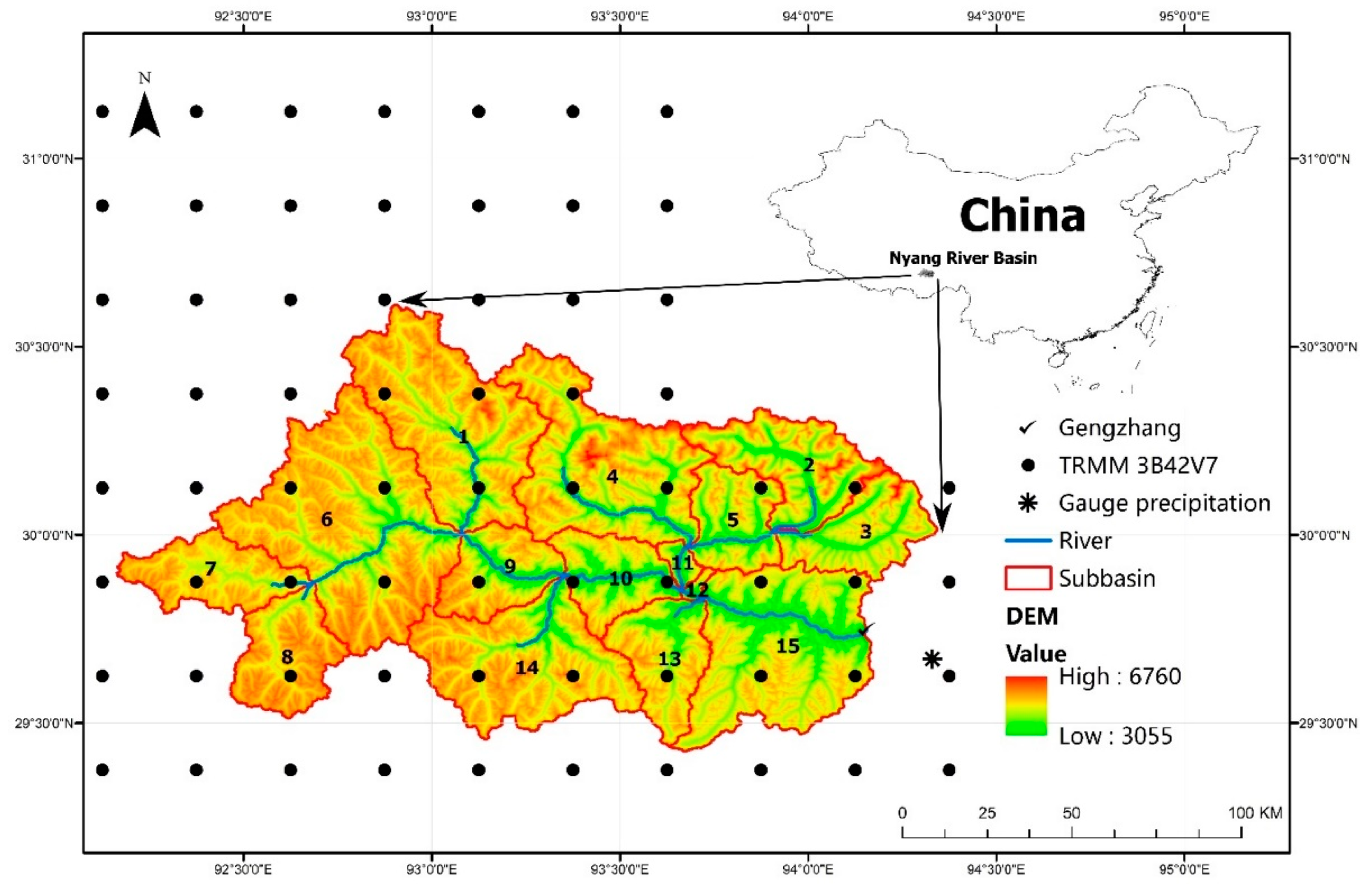
2.1. Study Area
2.2. Data
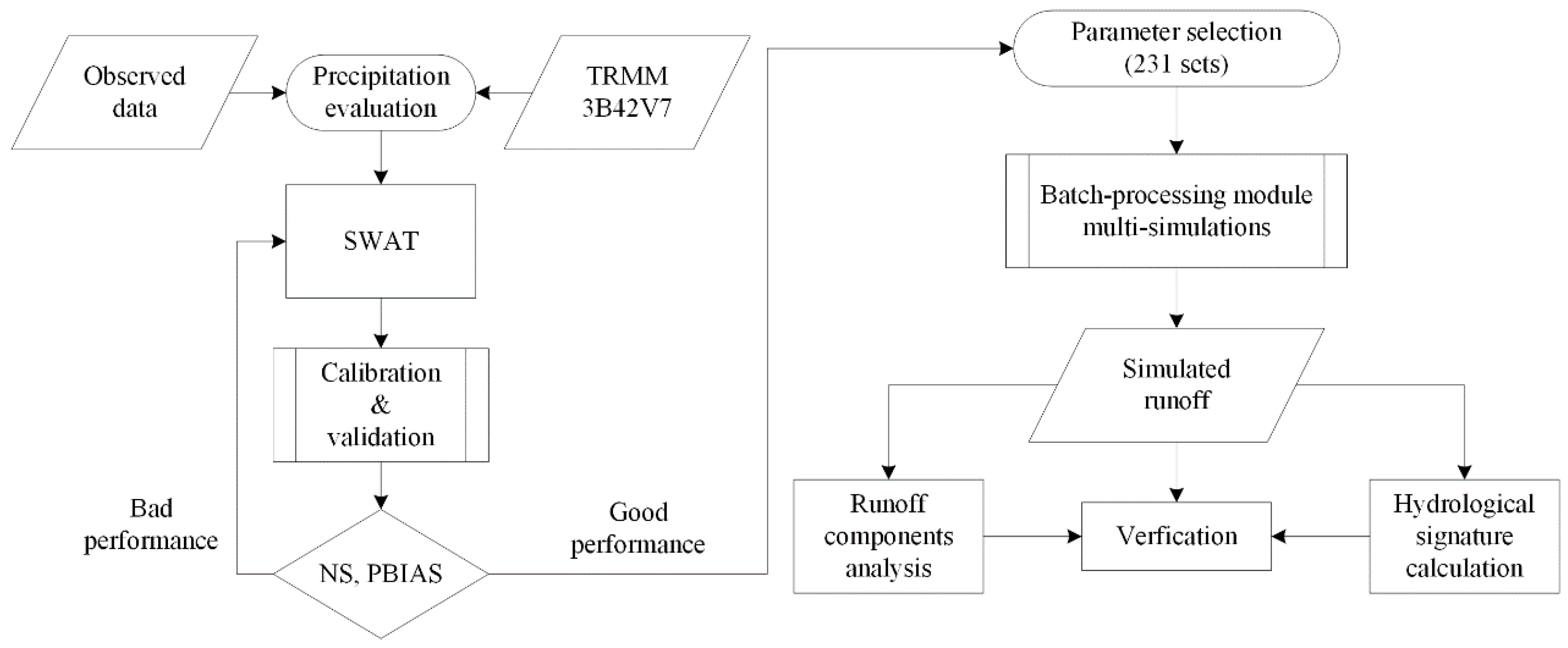
3. Methodology
3.1. Precipitation Evaluation Indices
3.2. Hydrological Model
3.3. Runoff Components and Hydrological Signatures
4. Results
4.1. Precipitation Evaluation Results
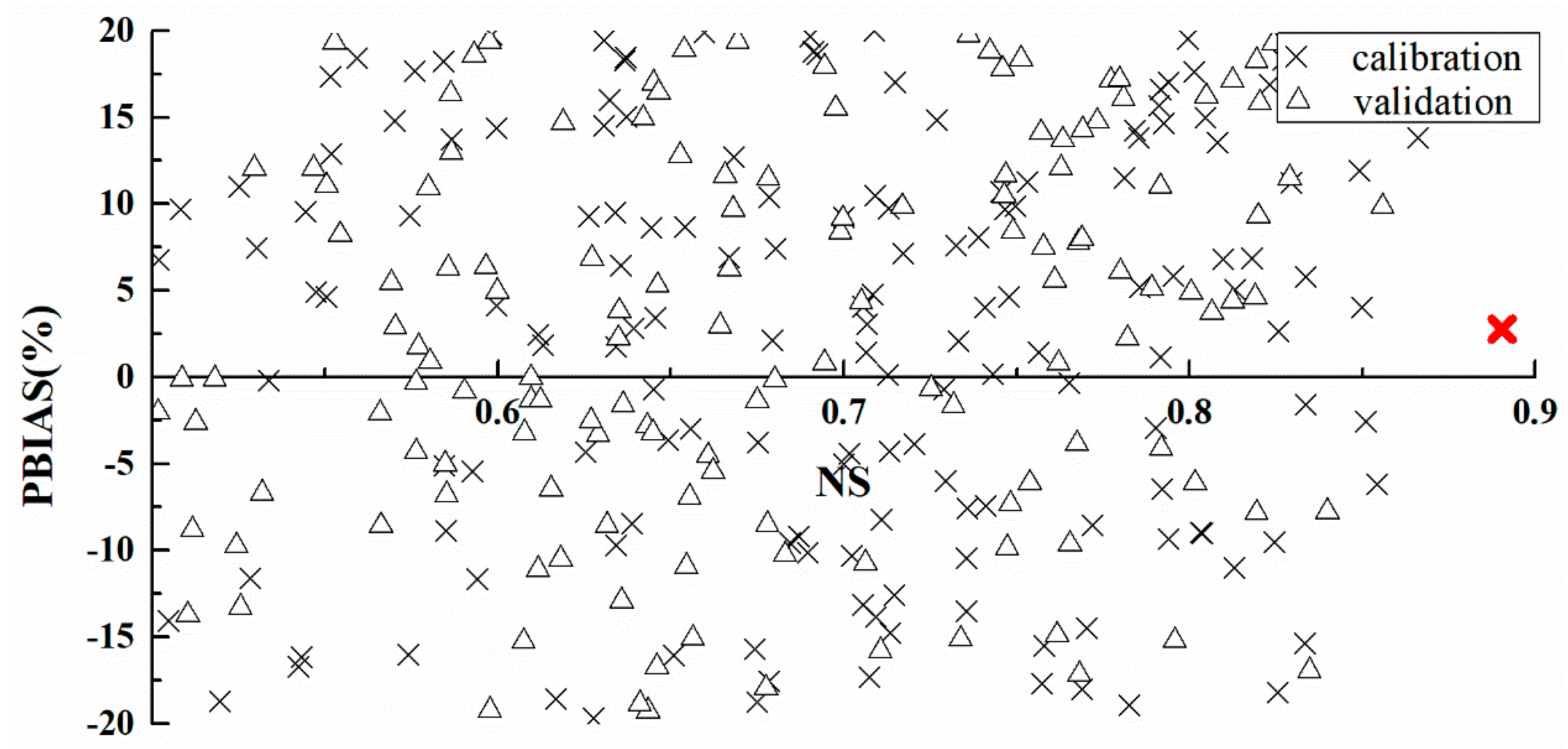
4.2. Hydrological Model Calibration and Validation
4.3. Runoff Component Analysis
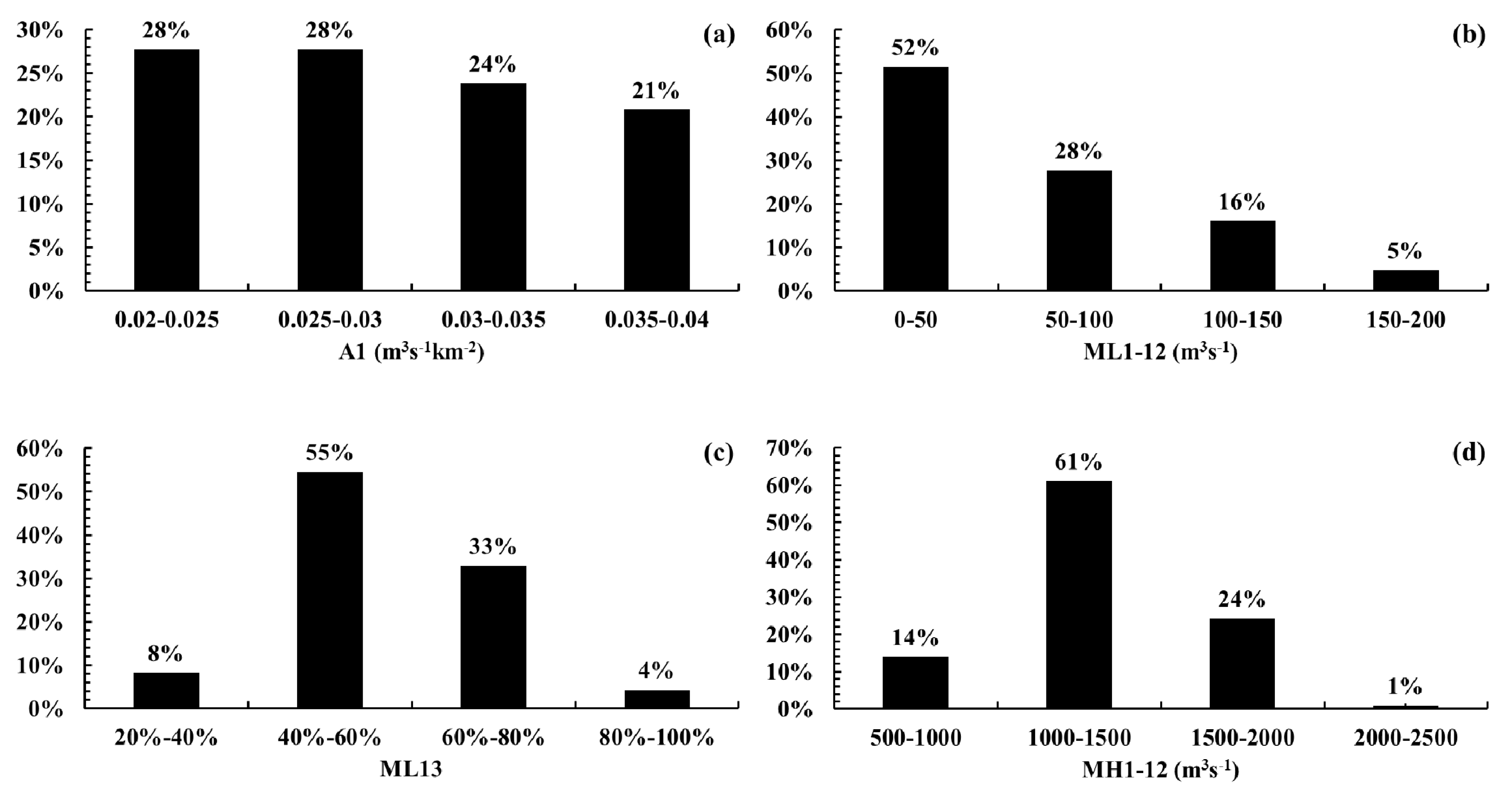
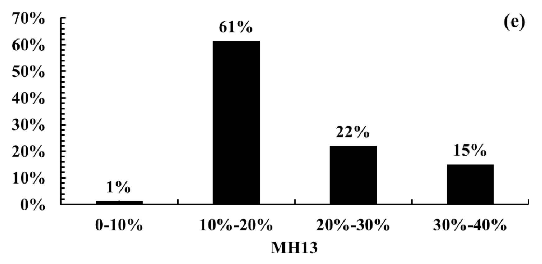
4.4. Hydrological Signatures
5. Discussion
6. Conclusions
Author Contributions
Funding
Conflicts of Interest
References
- Kaygusuz, K. Hydropower as clean and renewable energy source for electricity generation. J. Eng. Res. Appl. Sci. 2016, 5, 359–369. [Google Scholar]
- Oki, T.; Kanae, S. Global hydrological cycles and world water resources. Science 2006, 313, 1068–1072. [Google Scholar] [CrossRef] [PubMed]
- Haddeland, I.; Heinke, J.; Biemans, H.; Eisner, S.; Flörke, M.; Hanasaki, N.; Konzmann, M.; Ludwig, F.; Masaki, Y.; Schewe, J.; et al. Global water resources affected by human interventions and climate change. Proc. Natl. Acad. Sci. USA 2014, 111, 3251–3256. [Google Scholar] [CrossRef] [PubMed]
- Xu, X.; Lu, C.; Shi, X.; Gao, S. World water tower: An atmospheric perspective. Geophys. Res. Lett. 2008, 35, L20815. [Google Scholar] [CrossRef]
- Xue, X.; Hong, Y.; Limaye, A.S.; Gourley, J.J.; Huffman, G.J.; Khan, S.I.; Dorji, C.; Chen, S. Statistical and hydrological evaluation of TRMM-based Multi-satellite Precipitation Analysis over the Wangchu Basin of Bhutan: Are the latest satellite precipitation products 3B42V7 ready for use in ungauged basins? J. Hydrol. 2013, 499, 91–99. [Google Scholar] [CrossRef]
- Huffman, G.J.; Bolvin, D.T.; Nelkin, R.J.; Wolff, D.B.; Adler, R.F.; Gu, G.; Hong, Y.; Bowan, K.P.; Stocker, E.F. The TRMM multisatellite precipitation analysis (TMPA): Quasi-global, multiyear, combined-sensor precipitation estimates at fine scales. J. Hydrometeorol. 2007, 8, 38–55. [Google Scholar] [CrossRef]
- Joyce, R.J.; Janowiak, J.E.; Arkin, P.A.; Xie, P. CMORPH: A method that produces global precipitation estimates from passive microwave and infrared data at high spatial and temporal resolution. J. Hydrometeorol. 2004, 5, 487–503. [Google Scholar] [CrossRef]
- Sorooshian, S.; Hsu, K.L.; Gao, X.; Gupta, H.V.; Imam, B.; Braithwaite, D. Evaluation of PERSIANN system satellite-based estimates of tropical rainfall. Bull. Am. Meteorol. Soc. 2000, 81, 2035–2046. [Google Scholar] [CrossRef]
- Hong, Y.; Hsu, K.L.; Sorooshian, S.; Gao, X. Precipitation estimation from remotely sensed imagery using an artificial neural network cloud classification system. J. Appl. Meteorol. 2004, 43, 1834–1853. [Google Scholar] [CrossRef]
- Moazami, S.; Golian, S.; Kavianpour, M.R.; Hong, Y. Comparison of PERSIANN and V7 TRMM Multi-satellite Precipitation Analysis (TMPA) products with rain gauge data over Iran. Int. J. Remote Sens. 2013, 34, 8156–8171. [Google Scholar] [CrossRef]
- Yang, Y.; Luo, Y. Evaluating the performance of remote sensing precipitation products CMORPH, PERSIANN, and TMPA, in the arid region of northwest China. Theor. Appl. Climatol. 2014, 118, 429–445. [Google Scholar] [CrossRef]
- Zhu, Q.; Xuan, W.; Liu, L.; Xu, Y.P. Evaluation and hydrological application of precipitation estimates derived from PERSIANN-CDR, TRMM 3B42V7, and NCEP-CFSR over humid regions in China. Hydrol. Process. 2016, 30, 3061–3083. [Google Scholar] [CrossRef]
- Gupta, M.; Srivastava, P.K.; Islam, T.; Ishak, A.M.B. Evaluation of TRMM rainfall for soil moisture prediction in a subtropical climate. Environ. Earth Sci. 2014, 71, 4421–4431. [Google Scholar] [CrossRef]
- Prasetia, R.; As-syakur, A.R.; Osawa, T. Validation of TRMM Precipitation Radar satellite data over Indonesian region. Theor. Appl. Climatol. 2013, 112, 575–587. [Google Scholar] [CrossRef]
- Li, X.H.; Zhang, Q.; Xu, C.Y. Suitability of the TRMM satellite rainfalls in driving a distributed hydrological model for water balance computations in Xinjiang catchment, Poyang lake basin. J. Hydrol. 2012, 426, 28–38. [Google Scholar] [CrossRef]
- Landmann, T.; Dubovyk, O. Spatial analysis of human-induced vegetation productivity decline over eastern Africa using a decade (2001–2011) of medium resolution MODIS time-series data. Int. J. Appl. Earth Obs. Geoinf. 2014, 33, 76–82. [Google Scholar] [CrossRef]
- Zhang, A.; Jia, G. Monitoring meteorological drought in semiarid regions using multi-sensor microwave remote sensing data. Remote Sens. Environ. 2013, 134, 12–23. [Google Scholar] [CrossRef]
- Lang, T.J.; Barros, A.P. Winter storms in the central Himalayas. J. Meteorol. Soc. Jpn. 2004, 82, 829–844. [Google Scholar] [CrossRef]
- Barros, A.P.; Chiao, S.; Lang, T.J.; Burbank, D.; Putkonen, J. From weather to climate—Seasonal and interannual variability of storms and implications for erosion processes in the Himalaya. Geol. Soc. Am. Spec. Pap. 2006, 398, 17–38. [Google Scholar]
- Norris, J.; Carvalho, L.M.; Jones, C.; Cannon, F. WRF simulations of two extreme snowfall events associated with contrasting extratropical cyclones over the western and central Himalaya. J. Geophys. Res. Atmos. 2015, 120, 3114–3138. [Google Scholar] [CrossRef]
- Weiler, M.; Seibert, J.; Stahl, K. Magic components—Why quantifying rain, snowmelt, and icemelt in river discharge is not easy. Hydrol. Process. 2018, 32, 160–166. [Google Scholar] [CrossRef]
- Zhang, X.; Xu, Y.P.; Fu, G. Uncertainties in SWAT extreme flow simulation under climate change. J. Hydrol. 2014, 515, 205–222. [Google Scholar] [CrossRef]
- Abbaspour, K.C.; Rouholahnejad, E.; Vaghefi, S.; Srinivasan, R.; Yang, H.; Kløve, B. A continental-scale hydrology and water quality model for Europe: Calibration and uncertainty of a high-resolution large-scale SWAT model. J. Hydrol. 2015, 524, 733–752. [Google Scholar] [CrossRef]
- Cho, J.; Bosch, D.; Vellidis, G.; Lowrance, R.; Strickland, T. Multi-site evaluation of hydrology component of SWAT in the coastal plain of southwest Georgia. Hydrol. Process. 2013, 27, 1691–1700. [Google Scholar] [CrossRef]
- Fuka, D.R.; Collick, A.S.; Kleinman, P.J.; Auerbach, D.; Harmel, D.; Easton, Z.M. Improving the spatial representation of soil properties and hydrology using topographically derived initialization processes in the SWAT model. Hydrol. Process. 2016, 30, 4633–4643. [Google Scholar] [CrossRef]
- Han, H.D.; Ding, Y.J.; Liu, S.Y.; Wang, J. Regimes of runoff components on the debris-covered Koxkar glacier in western China. J. Mt. Sci. 2015, 12, 313–329. [Google Scholar] [CrossRef]
- Xing, B.; Liu, Z.; Liu, G.; Zhang, J. Determination of runoff components using path analysis and isotopic measurements in a glacier-covered alpine catchment (upper Hailuogou Valley) in southwest China. Hydrol. Process. 2015, 29, 3065–3073. [Google Scholar] [CrossRef]
- Olden, J.D.; Poff, N.L. Redundancy and the choice of hydrologic indices for characterizing streamflow regimes. River Res. Appl. 2003, 19, 101–121. [Google Scholar] [CrossRef]
- Yadav, M.; Wagener, T.; Gupta, H. Regionalization of constraints on expected watershed response behavior for improved predictions in ungauged basins. Adv. Water Res. 2007, 30, 1756–1774. [Google Scholar] [CrossRef]
- Yilmaz, K.K.; Gupta, H.V.; Wagener, T. A process-based diagnostic approach to model evaluation: Application to the NWS distributed hydrologic model. Water Resour. Res. 2008, 44. [Google Scholar] [CrossRef]
- Shafii, M.; Tolson, B.A. Optimizing hydrological consistency by incorporating hydrological signatures into model calibration objectives. Water Resour. Res. 2015, 51, 3796–3814. [Google Scholar] [CrossRef]
- Yong, B.; Ren, L.L.; Hong, Y.; Wang, J.H.; Gourley, J.J.; Jiang, S.H.; Chen, X.; Wang, W. Hydrologic evaluation of Multisatellite Precipitation Analysis standard precipitation products in basins beyond its inclined latitude band: A case study in Laohahe basin, China. Water Resour. Res. 2010, 46. [Google Scholar] [CrossRef]
- Abbaspour, K.C.; Yang, J.; Maximov, I.; Siber, R.; Bogner, K.; Mieleitner, J.; Zobrist, J.; Srinivasan, R. Modelling hydrology and water quality in the pre-alpine/alpine Thur watershed using SWAT. J. Hydrol. 2007, 333, 413–430. [Google Scholar] [CrossRef]
- Yang, J.; Reichert, P.; Abbaspour, K.C.; Xia, J.; Yang, H. Comparing uncertainty analysis techniques for a SWAT application to the Chaohe Basin in China. J. Hydrol. 2008, 358, 1–23. [Google Scholar] [CrossRef]
- Holvoet, K.; van Griensven, A.; Seuntjens, P.; Vanrolleghem, P.A. Sensitivity analysis for hydrology and pesticide supply towards the river in SWAT. Phys. Chem. Earth 2005, 30, 518–526. [Google Scholar] [CrossRef]
- Winchell, M.; Srinivasan, R.; Di Luzio, M.; Arnold, J. ArcSWAT Interface for SWAT2005 User’s Guide; Blackland Research and Extension Center: Temple, TX, USA, 2013; pp. 168–256. [Google Scholar]
- Abbaspour, K.C.; Johnson, C.A.; Van Genuchten, M.T. Estimating uncertain flow and transport parameters using a sequential uncertainty fitting procedure. Vadose Zone J. 2004, 3, 1340–1352. [Google Scholar] [CrossRef]
- Gupta, H.V.; Sorooshian, S.; Yapo, P.O. Status of automatic calibration for hydrologic models: Comparison with multilevel expert calibration. J. Hydrol. Eng. 1999, 4, 135–143. [Google Scholar] [CrossRef]
- Moriasi, D.N.; Arnold, J.G.; Van Liew, M.W.; Bingner, R.L.; Harmel, R.D.; Veith, T.L. Model evaluation guidelines for systematic quantification of accuracy in watershed simulations. Trans. ASABE 2007, 50, 885–900. [Google Scholar] [CrossRef]
- Nijssen, B.; Lettenmaier, D.P. Effect of precipitation sampling error on simulated hydrological fluxes and states: Anticipating the Global Precipitation Measurement satellites. J. Geophys. Res. Atmos. 2004, 109. [Google Scholar] [CrossRef]
- Abbaspour, C.K. SWAT Calibrating and Uncertainty Programs. A User Manual; Eawag: Zurich, Switzerland, 2015; pp. 17–66. [Google Scholar]
- Kampf, S.K.; Richer, E.E. Estimating source regions for snowmelt runoff in a Rocky Mountain basin: Tests of a data-based conceptual modeling approach. Hydrol. Process. 2014, 28, 2237–2250. [Google Scholar] [CrossRef]
- Arnold, J.G.; Muttiah, R.S.; Srinivasan, R.; Allen, P.M. Regional estimation of base flow and groundwater recharge in the Upper Mississippi river basin. J. Hydrol. 2000, 227, 21–40. [Google Scholar] [CrossRef]
- Qiu, L.J.; Zheng, F.L.; Yin, R.S. SWAT-based runoff and sediment simulation in a small watershed, the loessial hilly-gullied region of China: Capabilities and challenges. Int. J. Sediment. Res. 2012, 27, 226–234. [Google Scholar] [CrossRef]
- Luo, Y.; Arnold, J.; Allen, P.; Chen, X. Baseflow simulation using SWAT model in an inland river basin in Tianshan Mountains, Northwest China. Hydrol. Earth Syst. Sci. 2012, 16, 1259–1267. [Google Scholar] [CrossRef]
- Bharti, V.; Singh, C. Evaluation of error in TRMM 3B42V7 precipitation estimates over the Himalayan region. J. Geophy. Res. Atmos. 2015, 120, 12458–12473. [Google Scholar] [CrossRef]
- Maussion, F.; Scherer, D.; Mölg, T.; Collier, E.; Curio, J.; Finkelnburg, R. Precipitation seasonality and variability over the Tibetan Plateau as resolved by the High Asia Reanalysis. J. Clim. 2014, 27, 1910–1927. [Google Scholar] [CrossRef]
- The Climate Data Guide. TRMM: Tropical Rainfall Measuring Mission. Available online: https://climatedataguide.ucar.edu/climate-data/trmm-tropical-rainfall-measuring-mission (accessed on 26 October 2018).
- Bookhagen, B.; Burbank, D.W. Toward a complete Himalayan hydrological budget: Spatiotemporal distribution of snowmelt and rainfall and their impact on river discharge. J. Geophys. Res. Earth Surf. 2000, 115. [Google Scholar] [CrossRef]
- Chen, X.; Long, D.; Hong, Y.; Zeng, C.; Yan, D. Improved modeling of snow and glacier melting by a progressive two-stage calibration strategy with GRACE and multisource data: How snow and glacier meltwater contributes to the runoff of the Upper Brahmaputra River basin? Water Resour. Res. 2017, 53, 2431–2466. [Google Scholar] [CrossRef]
- Sun, C.; Chen, Y.; Li, X.; Li, W. Analysis on the streamflow components of the typical inland river, Northwest China. Hydrol. Sci. J. 2006, 61, 970–981. [Google Scholar] [CrossRef]


| Hydrological Signature | Code | Unit | Conditions | Definition |
|---|---|---|---|---|
| Mean annual runoff | A1 | m3 s−1 km−2 | Average flow conditions | Mean annual divided by catchment area |
| Mean minimum monthly flows | ML1-12 | m3 s−1 | Low flow conditions | Mean minimum monthly flow for all months |
| Variability across minimum monthly flows | ML13 | % | Low flow conditions | Coefficient of variation in minimum monthly flows |
| Mean maximum monthly flows | MH1-12 | m3 s−1 | High flow conditions | Mean of the maximum monthly flows for all months |
| Variability across maximum monthly flows | MH13 | % | High flow conditions | Coefficient of variation in maximum monthly flows |
| Code a | Parameter | Description | Unit | Initial Range |
|---|---|---|---|---|
| 1 | TLAPS v | Temperature lapse rate | °C km | [−10, 0] |
| 2 | PLAPS v | Precipitation lapse rate | mm/km | [−3, 3] |
| 3 | CN2 a | SCS runoff curve number for moisture condition 2 | - | [−57, 73] |
| 4 | SMTMP v | Snow melt base temperature | °C | [−5, 5] |
| 5 | SOL_Z r | Depth from soil surface to bottom of layer | mm | [−0.9, 150] |
| Item | A1 (m3 s−1 km−2) | ML1-12 (m3 s−1) | ML13 (%) | MH1-12 (m3 s−1) | MH13 (%) |
|---|---|---|---|---|---|
| Observation | 0.032 | 62.4 | 9 | 1557.4 | 16 |
| Upper | 0.021 | 3.1 | 30 | 752.9 | 10 |
| Median | 0.029 | 46.3 | 52 | 1305.1 | 17 |
| Lower | 0.040 | 166.8 | 87 | 1908.1 | 34 |
| “Best” | 0.027 | 67.3 | 62 | 1204.8 | 20 |
© 2018 by the authors. Licensee MDPI, Basel, Switzerland. This article is an open access article distributed under the terms and conditions of the Creative Commons Attribution (CC BY) license (http://creativecommons.org/licenses/by/4.0/).
Share and Cite
Xuan, W.; Fu, Q.; Qin, G.; Zhu, C.; Pan, S.; Xu, Y.-P. Hydrological Simulation and Runoff Component Analysis over a Cold Mountainous River Basin in Southwest China. Water 2018, 10, 1705. https://doi.org/10.3390/w10111705
Xuan W, Fu Q, Qin G, Zhu C, Pan S, Xu Y-P. Hydrological Simulation and Runoff Component Analysis over a Cold Mountainous River Basin in Southwest China. Water. 2018; 10(11):1705. https://doi.org/10.3390/w10111705
Chicago/Turabian StyleXuan, Weidong, Qiang Fu, Guanghua Qin, Cong Zhu, Suli Pan, and Yue-Ping Xu. 2018. "Hydrological Simulation and Runoff Component Analysis over a Cold Mountainous River Basin in Southwest China" Water 10, no. 11: 1705. https://doi.org/10.3390/w10111705
APA StyleXuan, W., Fu, Q., Qin, G., Zhu, C., Pan, S., & Xu, Y.-P. (2018). Hydrological Simulation and Runoff Component Analysis over a Cold Mountainous River Basin in Southwest China. Water, 10(11), 1705. https://doi.org/10.3390/w10111705