A New Well-Balanced Reconstruction Technique for the Numerical Simulation of Shallow Water Flows with Wet/Dry Fronts and Complex Topography

Abstract

This study develops a new well-balanced scheme for the one-dimensional shallow water system over irregular bed topographies with wet/dry fronts, in a Godunov-type finite volume framework. A new reconstruction technique that includes flooded cells and partially flooded cells and preserves the non-negative values of water depth is proposed. For the wet cell, a modified revised surface gradient method is presented assuming that the bed topography is irregular in the cell. For the case that the cell is partially flooded, this paper proposes a special reconstruction of flow variables that assumes that the bottom function is linear in the cell. The Harten–Lax–van Leer approximate Riemann solver is applied to evaluate the flux at cell faces. The numerical results show good agreement with analytical solutions to a set of test cases and experimental results.

1. Introduction

Non-linear shallow water equations, which can be derived by integrating the Euler equations in depth, have wide applications to surface flows, such as water flows of rivers, flood plains, practical dam failures, coastal regions and tides. Dam-breaks and floods may have enormous economic and human costs. Numerical solutions to the shallow water equations have been important in simulating floods and dam-break flows [1,2,3,4].

The present paper focuses on one-dimensional shallow water equation [5]:

$$\frac{\partial }{\partial t}\left[\begin{array}{c}h\\ hu\end{array}\right]+\frac{\partial }{\partial x}\left[\begin{array}{c}hu\\ h{u}^2+\frac{1}{2}g{h}^2\end{array}\right]=\left[\begin{array}{c}0\\ -gh\frac{\partial B}{\partial x}\end{array}\right]$$

(1)

where h(x, t) is the water depth, u(x, t) is the depth-averaged velocity, g is the gravitational constant, and B(x) is bottom topography. Subscripts denote partial derivatives. The friction system is ignored. The shallow water system can be written in vector form as

$$\frac{\partial \mathit{U}}{\partial t}+\frac{\partial \mathit{F}}{\partial x}=\mathit{S}$$

(2)

where U is the vector of conservable variables, F is the flux vector function, and S is the source vector, expressed as:

$$\mathit{U}=\left[\begin{array}{c}h\\ hu\end{array}\right],\hspace{1em}\mathit{F}=\left[\begin{array}{c}hu\\ h{u}^2+\frac{1}{2}g{h}^2\end{array}\right],\hspace{1em}\mathit{S}=\left[\begin{array}{c}0\\ -gh{B}_x\end{array}\right]$$

(3)

A large number of numerical schemes based on Equation (1) have been developed [6,7,8,9]. A challenge in developing a successful numerical scheme is to preserve the steady states at discrete levels. A scheme is called well-balanced if it is capable of balancing the flux and source terms exactly, which gives the motionless water surface in a lake [10,11]:

$$u=0,\hspace{1em}z=h+B=\mathrm{constant}$$

(4)

where z(x, t) is the water level. Many well-balanced schemes have been presented [12,13,14]. Another difficult issue is the presence of dry areas in the computational domain. In numerical oscillations, the water depth h may become negative near wet/dry fronts. The overall calculations then break down. Many numerical techniques that preserve the positive value of the water depth near wet/dry fronts have been put forward [15,16].

The surface gradient method (SGM) was proposed by Zhou et al. [17]. Compared with conventional data reconstruction methods based on the water depth, the SGM uses the water level as the basis of reconstruction. The advantage of the SGM used with source terms is that the SGM is generally suited to both steady and unsteady shallow water problems while the homogeneous terms are no more complicated than those of conventional methods. However, the SGM cannot be applied to shallow water flows over a vertical step and wet/dry fronts.

A modified surface gradient method (MSGM) was proposed using a fictitious cell at the vertical step by Zhou et al. [18]. Dae-Hong et al. [19] presented a revised surface gradient method (RSGM) assuming that the bottom topography in a grid is irregular rather than linear as in the SGM. However, the MSGM and RSGM cannot solve the wet/dry front with partially flooded cells. Kurganov and Levy [15] described a reconstruction adjustment for the partially flooded cell when the water depth becomes negative at integration points. Their correction ensures that the value of the water depth remains non-negative. However, the method is not well-balanced for very small water depth at flooded cells. Bollermann et al. [6] improved Kurganov’s method and proposed a well-balanced reconstruction method for the shallow water equations with wet/dry fronts.

In this study, we focus on the Godunov-type scheme and a reconstruction technique based on the values defined at the cell center. The Harten–Lax–van Leer (HLL) approximate Riemann solver is used to evaluate the flux terms at the cell interface. We present a robust, well-balanced and non-negative scheme that assumes the bottom function B(x) is continuous and linear only in partially flooded cells and the topography is irregular in flooded cells. The scheme proposes a modified RSGM and develops a new technique of reconstruction for partially flooded cells near the wet/dry fronts.

The remainder of the paper is organized as follows. The SGM and RSGM are reviewed briefly in Section 2. Section 3 describes the reconstruction method at the wet cell and the partially flooded cell. A Godunov-type method is introduced in Section 4. Several theoretical benchmark tests and laboratory dam-break problems are used to verify the performance of the proposed scheme in Section 5. Finally, conclusions are briefly presented in Section 6.

2. Review of the SGM and RSGM

In this section, the SGM and RSGM that are suitable for flooded cells are briefly reviewed. A uniform grid with finite volume $I_i:\left[x_{i-1/2},x_{i+1/2}\right]$ of length $\Delta x$ is used. The cell-averaged value $\overline{\mathit{U}}$ is expressed by $\overline{\mathit{U}}{\left(t\right)}_i=\frac{1}{\Delta x}{\displaystyle {\int }_{I_i}\mathit{U}}\left(x,t\right)dx$, where $\mathit{U}={\left(h,hu\right)}^{\mathrm{T}}$. Apparently, in the flooded cell, ${\overline{\mathit{U}}}_i\left(x,t\right)={\left({\overline{h}}_i,\overline{h_i{u}_i}\right)}^{\mathrm{T}}$ is the same as ${\mathit{U}}_i\left(x,t\right)={\left(h_i,h_i{u}_i\right)}^{\mathrm{T}}$.

2.1. SGM

In high-order accurate Godunov-type schemes, the values at the cell interface are computed by reconstruction based on data at the cell center. The monotone upstream-centered scheme for conservation laws (MUSCL) approach, which has second-order accuracy in space resulting from piecewise linear reconstruction from values defined at cell center, is widely applied in the framework of Godunov-type schemes [3,4].

For the continuity Equation (1), the water level $z$ at the cell center is chosen to be reconstructed in the SGM. The water level $z$ within a cell can be expressed as

$$z(x,t)=z_i+(x-x_i)\delta z_i$$

(5)

and the water depth $h$ within a cell is

$$h(x,t)=z(x,t)-B(x)=z_i+(x-x_i)\delta z_i-B(x)$$

(6)

where $\delta z_i$ is the gradient of $z$, calculated as

$$\delta z_i=G(\frac{z_{i+1}-z_i}{x_{i+1}-x_i},\frac{z_i-z_{i-1}}{x_i-x_{i-1}})$$

(7)

in which $G$ is a slope limiter that avoids the generation of spurious oscillations in the process of reconstruction at the cell interface. Researchers have proposed several slope limiters that have been demonstrated to have good performance in numerical experiments [20], such as the minmod limiter, van Leer limiter, and superbee limiter. Here, the minmod limiter, which is expressed as

$$G\left(a,b\right)=\max \left[0,\min \left(a,b\right)\right]$$

(8)

is selected. The values of $z$ at the interfaces in a cell are

$$z_{i-\frac{1}{2}}^R=z_i-\frac{1}{2}\Delta x_i\delta z_i,\hspace{1em}{z}_{i+\frac{1}{2}}^L=z_i+\frac{1}{2}\Delta x_i\delta z_i,\hspace{1em}\Delta x_i=x_{i+\frac{1}{2}}-x_{i-\frac{1}{2}}$$

(9)

and the values of water depth $h$ at interfaces in a cell are

$$\begin{array}{l}{h}_{i-\frac{1}{2}}^R=z_{i-\frac{1}{2}}^R-B_{i-\frac{1}{2}}=z_i-\frac{1}{2}\Delta x_i\delta z_i-B_{i-\frac{1}{2}}\\ h_{i+\frac{1}{2}}^L=z_{i+\frac{1}{2}}^L-B_{i+\frac{1}{2}}=z_i+\frac{1}{2}\Delta x_i\delta z_i-B_{i+\frac{1}{2}}\end{array}$$

(10)

The bed topography is defined at the cell interface and is assumed to have a piecewise profile within a cell in the SGM. The bed topography at the cell center is then expressed exactly as

$$B_i=\frac{1}{2}(B_{i-\frac{1}{2}}+B_{i+\frac{1}{2}})$$

(11)

For the momentum equation in Equation (1), the conserved value $hu$ is selected to be reconstructed and the solution can be formulated in a similar manner to the formulation for $z$. For the stationary case $u=0$ and $z=\mathrm{constant}$, which is the “lake at rest” steady state, the momentum flux in Equations (1) is discretized using a Godunov-type scheme as

$$\frac{\partial F}{\partial x}=\frac{{(h{u}^2+\frac{1}{2}g{h}^2)}_{i+\frac{1}{2}}-{(h{u}^2+\frac{1}{2}g{h}^2)}_{i-\frac{1}{2}}}{\Delta x}=\frac{g}{2\Delta x}(h_{i+\frac{1}{2}}+h_{i-\frac{1}{2}})(h_{i+\frac{1}{2}}-h_{i-\frac{1}{2}})$$

(12)

Under the condition $z=\mathrm{constant}$, the value of $\delta z_i$ becomes zero and Equation (10) becomes

$$\frac{h_{i-\frac{1}{2}}+h_{i+\frac{1}{2}}}{2}=\frac{z_{i-\frac{1}{2}}+z_{i+\frac{1}{2}}-(B_{i-\frac{1}{2}}+B_{i+\frac{1}{2}})}{2}=z_i-\frac{(B_{i-\frac{1}{2}}+B_{i+\frac{1}{2}})}{2}$$

(13)

According to Equation (11), Equation (13) can be rewritten as

$$\frac{h_{i-\frac{1}{2}}+h_{i+\frac{1}{2}}}{2}=z_i-\frac{(B_{i-\frac{1}{2}}+B_{i+\frac{1}{2}})}{2}=z_i-B_i=h_i$$

(14)

Equation (12) then becomes

$$\frac{\partial F}{\partial x}=\frac{g}{2\Delta x}(h_{i+\frac{1}{2}}+h_{i-\frac{1}{2}})(h_{i+\frac{1}{2}}-h_{i-\frac{1}{2}})=\frac{g}{\Delta x}{h}_i(h_{i+\frac{1}{2}}-h_{i-\frac{1}{2}})$$

(15)

At the same time, the source term, which is the bed slope term of the momentum Equation (1), is discretized as

$$S=-g{h}_i\frac{B_{i+\frac{1}{2}}-B_{i-\frac{1}{2}}}{\Delta x}=\frac{g}{\Delta x}{h}_i(B_{i-\frac{1}{2}}-B_{i+\frac{1}{2}})=\frac{g}{\Delta x}{h}_i(h_{i+\frac{1}{2}}-h_{i-\frac{1}{2}})$$

(16)

Note that $B_{i-\frac{1}{2}}-B_{i+\frac{1}{2}}=h_{i+\frac{1}{2}}-h_{i-\frac{1}{2}}$, because the water level $z$ is constant throughout the computational domain.

From Equations (15) and (16), it is concluded that $\partial F/\partial x=S$, which means the SGM satisfies the exact C-property and can be called a well-balanced scheme.

2.2. RSGM

As presented in Equations (11) and (14), the SGM assumes that the arithmetic mean of the water depth at the two interfaces of a cell is the same as the water depth at the cell center of a cell. However, in the case of the RSGM, Dae-Hong Kim et al. pointed out that the assumption is valid only when the bottom slope of the cell is constant [19]. For irregular bathymetry, the SGM may produce unwanted computational results.

In the RSGM, Equation (14) is rewritten as

$$\frac{h_{i-\frac{1}{2}}+h_{i+\frac{1}{2}}}{2}=z_i-\frac{(B_{i-\frac{1}{2}}+B_{i+\frac{1}{2}})}{2}=h_i+B_i-\frac{(B_{i-\frac{1}{2}}+B_{i+\frac{1}{2}})}{2}$$

(17)

because Equation (11) is not satisfied in general cases. Furthermore, Equation (15) becomes

$$\frac{\partial F}{\partial x}=\frac{g}{2\Delta x}(h_{i+\frac{1}{2}}+h_{i-\frac{1}{2}})(h_{i+\frac{1}{2}}-h_{i-\frac{1}{2}})$$

(18)

To balance the flux term and source term in the stationary case, $F$ in Equation (18) should be the same as the source term when it is discretized using a central discretization scheme in a cell:

$$\begin{array}{l}\frac{\partial F}{\partial x}=\frac{g}{2\Delta x}(h_{i+\frac{1}{2}}+h_{i-\frac{1}{2}})(h_{i+\frac{1}{2}}-h_{i-\frac{1}{2}})=S\\ =\frac{g}{\Delta x}h(B_{i-\frac{1}{2}}-B_{i+\frac{1}{2}})=\frac{g}{\Delta x}h(h_{i+\frac{1}{2}}-h_{i-\frac{1}{2}})\end{array}$$

(19)

From Equation (19), a new arithmetic formula is obtained:

$$\frac{h_{i+\frac{1}{2}}+h_{i-\frac{1}{2}}}{2}=h$$

(20)

Equation (20) is similar to Equation (14) but has different implications; i.e., the water depth $h$ in the source term should be discretized as $(h_{i+\frac{1}{2}}+h_{i-\frac{1}{2}})/2$, rather than $h_i$. Finally, the source term is discretized as

$$S=-gh\frac{B_{i+\frac{1}{2}}-B_{i-\frac{1}{2}}}{\Delta x}=\frac{g}{\Delta x}h(B_{i-\frac{1}{2}}-B_{i+\frac{1}{2}})=\frac{g}{\Delta x}\frac{(h_{i+\frac{1}{2}}+h_{i-\frac{1}{2}})(h_{i+\frac{1}{2}}-h_{i-\frac{1}{2}})}{2}$$

(21)

The reconstruction for the conserved value of $hu$ is the same as the solution in the SGM. Further details have been given by Zhou et al. [17] and Dae-Hong Kim et al. [19].

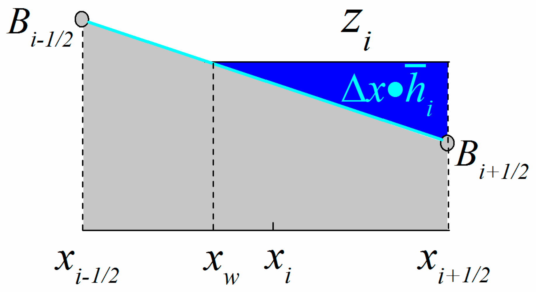
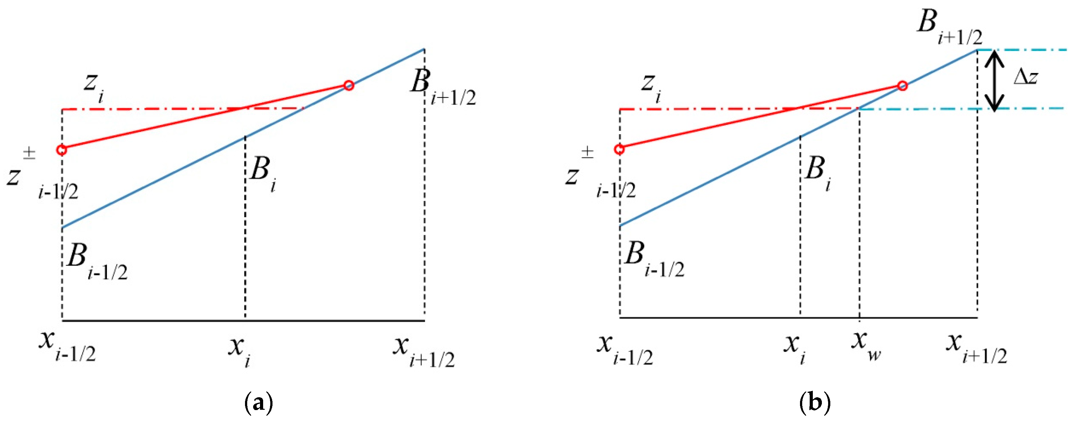
3. New Reconstruction Technique

We assume that all the computed values $h_i$ are positive at a certain time step.

3.1. Reconstruction for the Flooded Cell

The flooded cell should satisfy

$$z_i>B_{i+\frac{1}{2}} \mathrm{and} z_i>B_{i-\frac{1}{2}}$$

(22)

For the flooded cell, the reconstruction method of the RSGM, which assumes that the bottom topography is irregular, is applied. In Section 2, we introduced the SGM and RSGM briefly. After the reconstruction, the values of $h_{i+1/2}^{-}$ or $h_{i-1/2}^{+}$ may be negative (Figure 1b), even though the average water depth $h_i$ is positive (Figure 1a). The RSGM is therefore modified as follows.

Figure 1. Correction for negative values of $h_{i+1/2}^{-}$ and $h_{i-1/2}^{+}$. (a) After the reconstruction, the water depth $h_{i-1/2}^{+}$ is negative at the right side of the i − 1/2 interface; (b) the average water depth $h_i$ is positive; (c) the correction result. We reset $z_{i-1/2}^{+}=B_{i-1/2},h_{i-1/2}^{+}=0$. $z_{i+1/2}^{-}$ also needs to be corrected considering the conservation of the total amount of water.

(1)

If $h_{i+1/2}^{-}$ and $h_{i-1/2}^{+}$ are both positive, the RSGM is applied.

(2)

If $z_{i-1/2}^{+}<B_{i-1/2}$, we reset the water level at the two sides of the cell (Figure 1c):

$$z_{i-1/2}^{+}=B_{i-1/2},\hspace{1em}{z}_{i+1/2}^{-}=2z_i-z_{i-1/2}^{+}$$

(23)

(3)

If $z_{i+1/2}^{-}<B_{i+1/2}$, a similar correction is made.

3.2. Reconstruction at the Partially Flooded Cell

We assume the bottom topography function is linear in the partially flooded cell. The partially flooded cell, which has a dry area in the cell (Figure 2), may produce negative values of the water depth at cell interfaces in the reconstruction stage introduced in Section 2. In Figure 2, $x_w$ is the separation point between wet and dry areas. Here, we note that $\overline{U}\ne U$ in the partially flooded cell. The water level function $z\left(x\right)$ is defined as

$$z_i(x)=\{\begin{array}{ll}{z}_i& \mathrm{if} x>x_w\\ B_i(x)& \mathrm{if} x<x_w\end{array}$$

(24)

Figure 2. Partially flooded cell.

The total amount of water given by $\Delta x\cdot {\overline{h}}_i$ is equal to the volume enclosed between the water level line and the bathymetry. Then, if cell $i$ is fully flooded, it satisfies the condition

$${\overline{h}}_i\ge \frac{\left|B_{i-1/2}-B_{i+1/2}\right|}{2}=\frac{\Delta x}{2}\left|{(B_x)}_i\right|$$

(25)

where $\left|{(B_x)}_i\right|$ is the bed slope in cell $i$. The separation point $x_w$ can be derived from mass conservation:

$$\begin{array}{cc}\hfill \Delta x\cdot {\overline{h}}_i& ={\displaystyle \underset{x_{i-1/2}}{\overset{x_{i+1/2}}{\int }}(z_i(x)-B_i(x))}dx={\displaystyle \underset{x_w}{\overset{x_{i+1/2}}{\int }}(z_i(x)-B_i(x))}dx\hfill \\ & =\frac{\Delta x_w}{2}(z_i-B_{i+1/2})=\frac{\Delta x_w}{2}(B_{x_w}-B_{i+1/2})\hfill \\ & =\frac{{\left(\Delta x_w\right)}^2}{2}\left|{(B_x)}_i\right|\hfill \end{array}$$

(26)

where $\Delta x_w=x_{i+1/2}-x_w$. Thus,

$$\Delta x_w=\sqrt{\frac{2\Delta x\cdot {\overline{h}}_i}{\left|{(B_x)}_i\right|}}\le \Delta x$$

(27)

The formula for the free surface is

$$z_i=B_{i+1/2}+\sqrt{2\overline{h_i}\left|B_{i-1/2}-B_{i+1/2}\right|}$$

(28)

For the partially flooded cell, we modify the water depth values $h_{i-1/2}^{+}$ and $h_{i+1/2}^{-}$ at cell interfaces obtained in the reconstruction step. First, we define that the water depth value $z_{i-1/2}^{-}$ reconstructed in the next flooded cell equals $z_{i-1/2}^{+}$ [6]. Immediately, it follows that $h_{i-1/2}^{-}=h_{i-1/2}^{+}$. Two cases are considered.

Case 1.

If there is sufficient water, then $h_{i+1/2}^{-}\ge 0$ and, from Figure 3

$$\overline{h_i}=\frac{1}{2}(h_{i-1/2}^{+}+h_{i+1/2}^{-})$$

(29)

Figure 3. Linear reconstruction with positive $h_{i+1/2}^{-}$ for the partially flooded cell with sufficient water.

From Equation (29), we obtain

$$h_{i+1/2}^{-}=2\overline{h_i}-h_{i-1/2}^{+}$$

(30)

The water level $z_{i+1/2}^{-}=h_{i+1/2}^{-}+B_{i+1/2}$, and the well-balanced reconstruction in partially flooded cell $i$ is complete.

Case 2.

If $h_{i+1/2}^{-}<0$ computed from Equation (30) (Figure 4a), the reconstruction step is neglected in cell $i$. We replace the water level and water depth values at the $i+1/2$ interface by those at the $x_w$ interface:

$$\begin{array}{l}{h}^{-}{}_{x_w}=h^{-}{}_{i+1/2}=0\\ z^{-}{}_{x_w}=z^{-}{}_{i+1/2}=B_{x_w}\end{array}$$

(31)

where $x_w$ is obtained using Equation (27). To keep the well-balanced property, the value $z^{+}{}_{i+1/2}$ is subtracted from $\Delta z$ (Figure 4b):

$$\begin{array}{l}{h}^{+}{}_{i+1/2}=0\\ \Delta z=z^{+}{}_{i+1/2}-z^{+}{}_{x_w}\\ z^{+}{}_{i+1/2}=z^{+}{}_{i+1/2}-\Delta z=B_{x_w}\end{array}$$

(32)

Figure 4. Linear reconstruction with negative $h^{-}{}_{i+1/2}$ for the partially flooded cell. (a) Without correction; (b) correction of values at the i + 1/2 interface.

Here we make two statements about the new reconstruction technique: (1) If the cell is fully flooded satisfying Equation (22), the modified RSGM presented in Section 3.1 is applied; (2) when the cell does not satisfy the conditions of Equation (22) or Equation (25), the cell is partially flooded. Two practical cases are considered in Section 3.2.

4. Implementation Using a Godunov-Type Method

The reconstruction method proposed in this paper can be incorporated into any Godunov-type method that requires data reconstruction. Here, the MUSCL method having second-order accuracy in space is used. The updating conservative formula is

$${\overline{\mathit{U}}}_i^{n+1}={\overline{\mathit{U}}}_i^n-\frac{\Delta t}{\Delta x}\left[{\mathit{F}}_{i+1/2}^{\mathrm{HLL}}-{\mathit{F}}_{i-1/2}^{\mathrm{HLL}}\right]+\Delta t\overline{{\mathit{S}}_i}$$

(33)

where ${\mathit{F}}_{i+1/2}^{\mathrm{HLL}}$ and ${\mathit{F}}_{i-1/2}^{\mathrm{HLL}}$ are fluxes at cell interfaces. The HLL approximate Riemann solver is determined by

$${\mathit{F}}_{i+1/2}^{\mathrm{HLL}}=\{\begin{array}{ll}{\mathit{F}}_L& \mathrm{if}{S}_L\ge 0\\ {\mathit{F}}^{\mathrm{HLL}}=\frac{S_R{\mathit{F}}_L-S_L{\mathit{F}}_R+S_R{S}_L({\mathit{U}}_R-{\mathit{U}}_L)}{S_R-S_L}& \mathrm{if}{S}_L\le 0\le S_R\\ {\mathit{F}}_R& \mathrm{if}{S}_R\le 0\end{array}$$

(34)

and wave speeds S are given by

$$\begin{array}{l}{S}_L=\{\begin{array}{ll}\min (u_L-\sqrt{g{h}_L},u_{\ast }-\sqrt{g{h}_{\ast }})& \mathrm{if} h_L>0\\ u_R-2\sqrt{g{h}_R}& \mathrm{if} h_L=0\end{array}\\ S_R=\{\begin{array}{ll}\max (u_R+\sqrt{g{h}_R},u_{\ast }+\sqrt{g{h}_{\ast }})& \mathrm{if} h_R>0\\ u_L+2\sqrt{g{h}_L}& \mathrm{if} h_R=0\end{array}\end{array}$$

(35)

where

$$\begin{array}{l}{h}_{\ast }=\frac{\left(u_L+2\sqrt{g{h}_L}-u_R-2\sqrt{g{h}_R}\right)}{16g}\\ u_{\ast }=\frac{u_L+u_R}{2}+\sqrt{g{h}_L}-\sqrt{g{h}_R}\end{array}$$

(36)

$\overline{S_i}$ denotes the source term. If the cell is flooded, according to Equation (21) applied in the RSGM, the source term is discretized as

$$\begin{array}{cc}\hfill \overline{S_i}& =-gh\frac{B_{i+\frac{1}{2}}-B_{i-\frac{1}{2}}}{\Delta x}=\frac{g}{\Delta x}h(B_{i-\frac{1}{2}}-B_{i+\frac{1}{2}})\hfill \\ & =\frac{g}{\Delta x}\frac{(h_{i+\frac{1}{2}}+h_{i-\frac{1}{2}})(B_{i-\frac{1}{2}}-B_{i+\frac{1}{2}})}{2}\hfill \end{array}$$

(37)

If the cell is partially flooded, in which the bottom topography function is assumed to be linear, according to Equation (16) applied in the SGM, the source term is discretized as

$$\overline{S_i}=-g{h}_i\frac{B_{i+\frac{1}{2}}-B_{i-\frac{1}{2}}}{\Delta x}=\frac{g}{\Delta x}{h}_i(B_{i-\frac{1}{2}}-B_{i+\frac{1}{2}})$$

(38)

To prevent numerical instability near dry areas, the average velocity is defined by

$$\overline{u_i}=\{\begin{array}{ll}\frac{{(\overline{hu})}_i}{\overline{h_i}}& \mathrm{if} \overline{h_i}>{10}^{-6} m\\ 0& \mathrm{othwewise}\end{array}$$

(39)

The time step $\Delta t$ is determined by the Courant-Friedrichs-Lewy (CFL) condition:

$$\begin{array}{l}\Delta t=\frac{C_{cfl}\cdot \Delta x}{\max (\left|{\overline{u_i}}^n\right|+\sqrt{g\overline{h_i^n}})}\\ 0<C_{cfl}\le 1\end{array}$$

(40)

where $C_{cfl}$ is the Courant number. $C_{cfl}=0.5$ is used in this paper.

5. Numerical Results

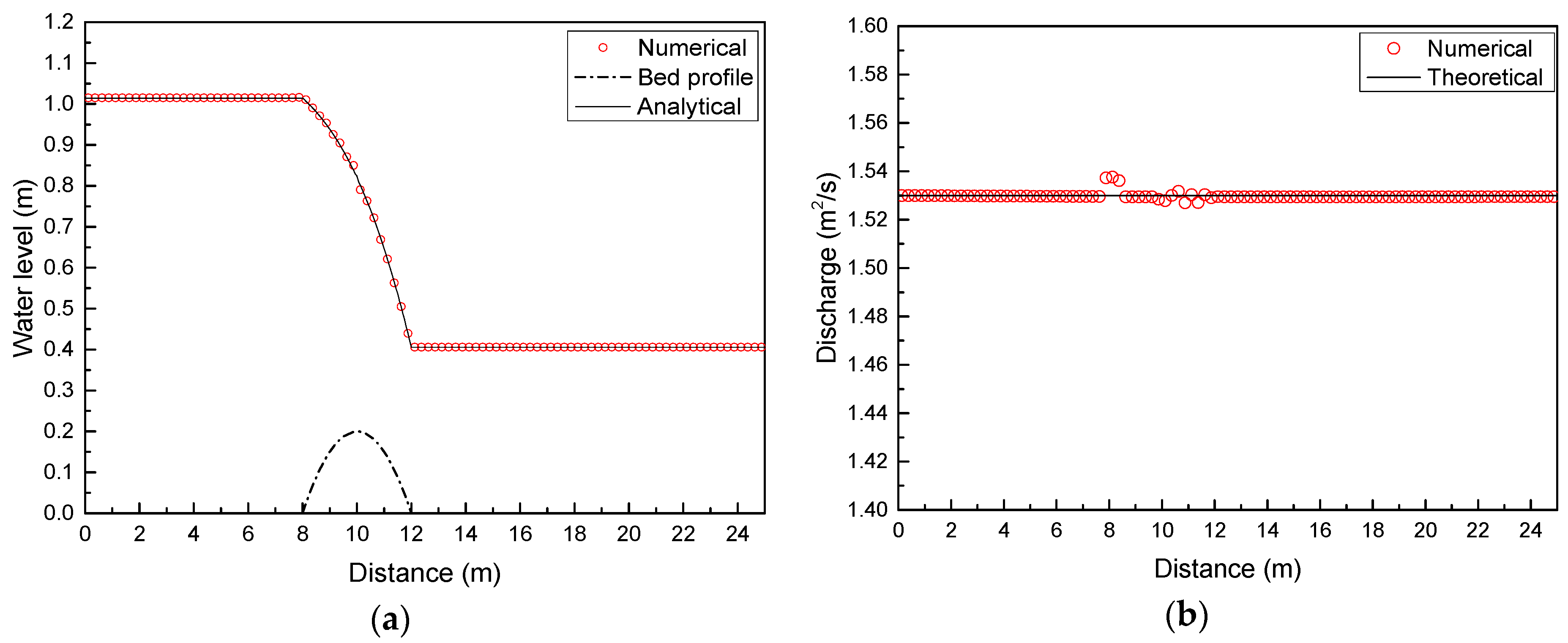
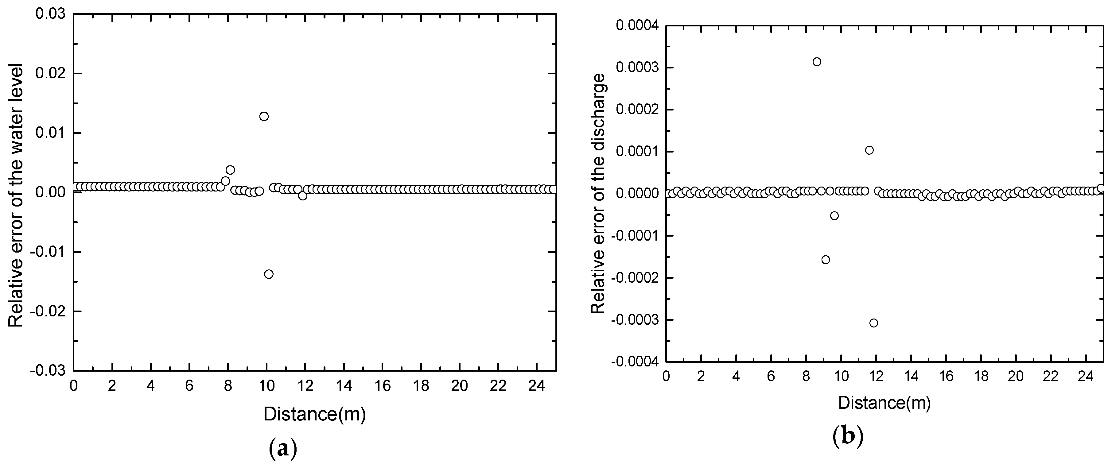
5.1. Steady Flow over One-Bump Topography

Steady flow with one-bump topography is tested in a 25-m-long channel. The bathymetry is defined as

$$B(x)=\{\begin{array}{ll}0.2-0.05{(x-10)}^2& \mathrm{if} 8 \mathrm{m}<x<12 \mathrm{m}\\ 0.0& \mathrm{otherwise}\end{array}$$

(41)

Four cases are considered in testing the proposed scheme.

5.1.1. Still-Water Test for Well-Balanced Property

The first test is of the property to preserve the “lake at rest” in Equation (4) with wet/dry interfaces and 100 uniform cells. The initial water level is given by $z_x=\max \left(0.1,B\left(x\right)\right)$ so that the bump is partially submerged. Simulations run for 500 s and the result is shown in Figure 5. The still water level remains unchanged and meets the analytical solution perfectly.

Figure 5. Still-water test after 500 s.

5.1.2. Transcritical Flow without a Shock

The unit discharge q = 1.53 m²/s is imposed at the upstream boundary and zero gradient condition is given at the downstream boundary. The initial water level and velocity are 0.4 m and 0 m/s, respectively. There are 100 computational cells. Figure 6 compares the numerical results and analytical solution. The surface profile has good agreement with the analytical solution. Furthermore, the comparison between the computed discharge and the theoretical results shows that the scheme is conservative. The relative error is given in Figure 7.

Figure 6. Transcritical flow without a shock over a bump: (a) comparison of the water level between numerical results and the analytical solution; (b) comparison of discharge.

Figure 7. Transcritical flow without a shock over a bump. The relative error: (a) the water level z; (b) the discharge q = hu.

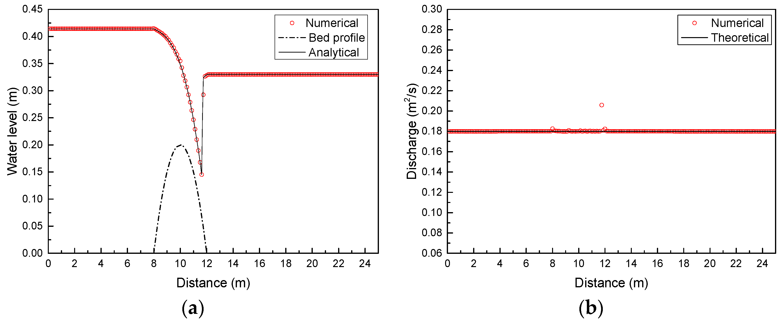
5.1.3. Transcritical Flow with a Shock

The unit discharge q = 0.18 m²/s is imposed at the upstream boundary and h = 0.33 m is given at the downstream boundary. The number of computational cells is 200. Figure 8 compares the computational results with the analytical solution. The relative error is given in Figure 9.

Figure 8. Transcritical flow with a shock over a bump: (a) comparison of the water level between numerical results and the analytical solution; (b) comparison of discharge.

Figure 9. The relative error of transcritical flow with a shock over a bump: (a) the water level z; (b) the discharge q = hu.

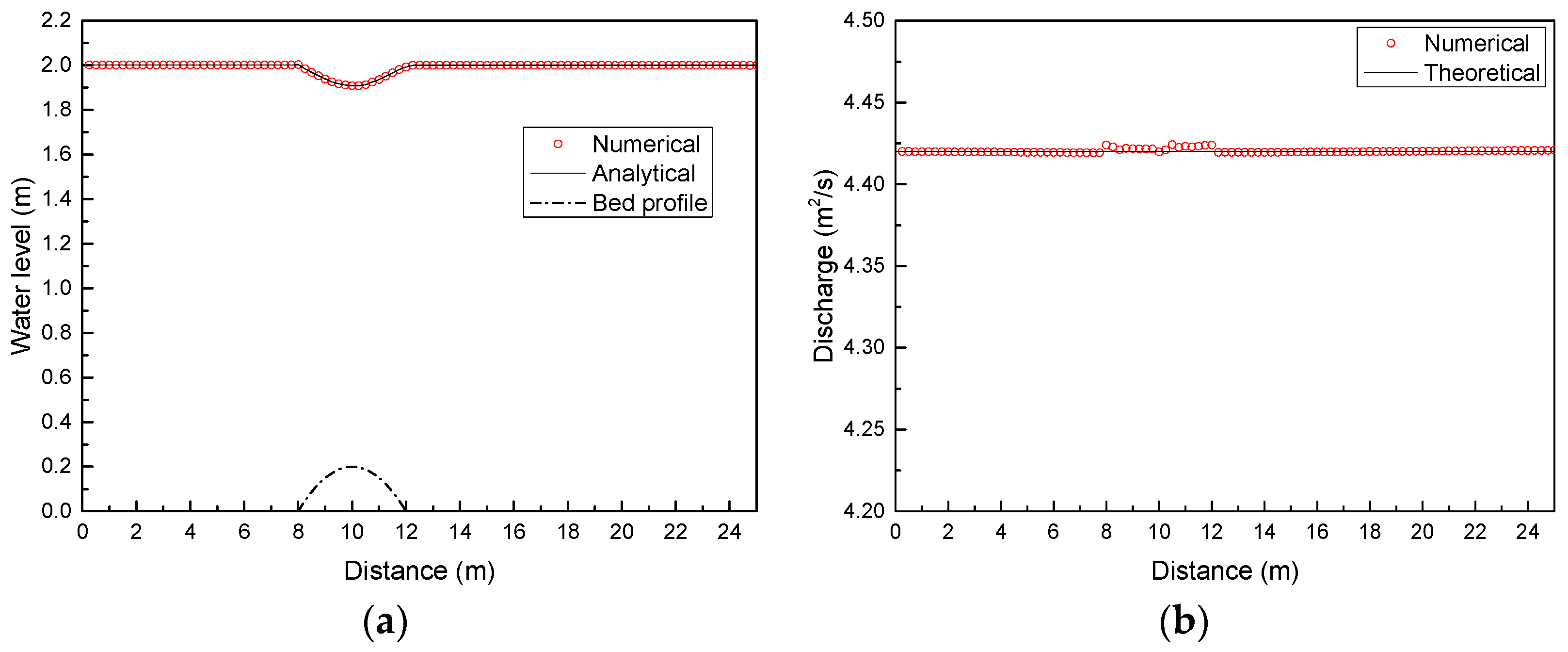
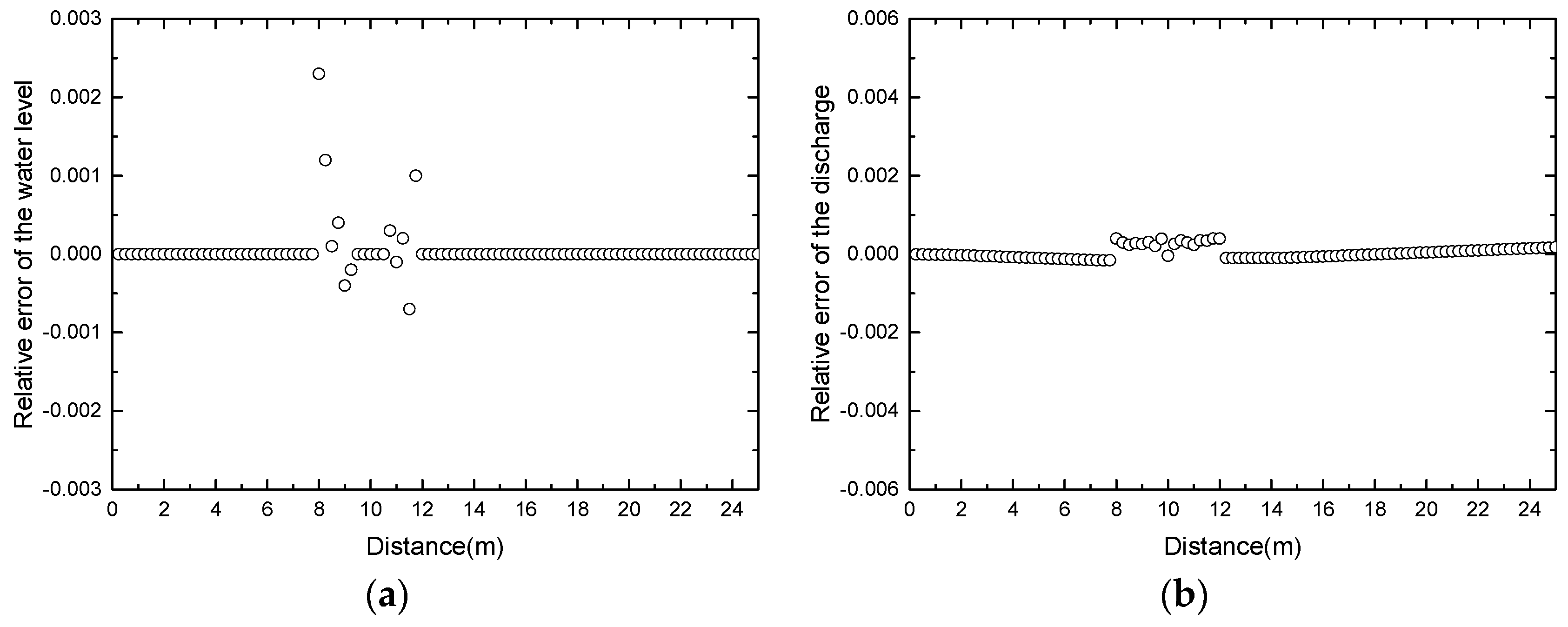
5.1.4. Subcritical Flow

A unit discharge q = 4.42 m²/s is imposed at the upstream boundary and h = 2 m is specified at the downstream boundary. The number of computational cells is 100. The numerical results are depicted in Figure 10 and have excellent agreement with the analytical solution. The relative error is given in Figure 11.

Figure 10. Subcritical flow over a bump: (a) comparison of the water level between numerical results and the analytical solution; (b) comparison of discharge.

Figure 11. The relative error of subcritical flow over a bump: (a) the water level z; (b) the discharge q = hu.

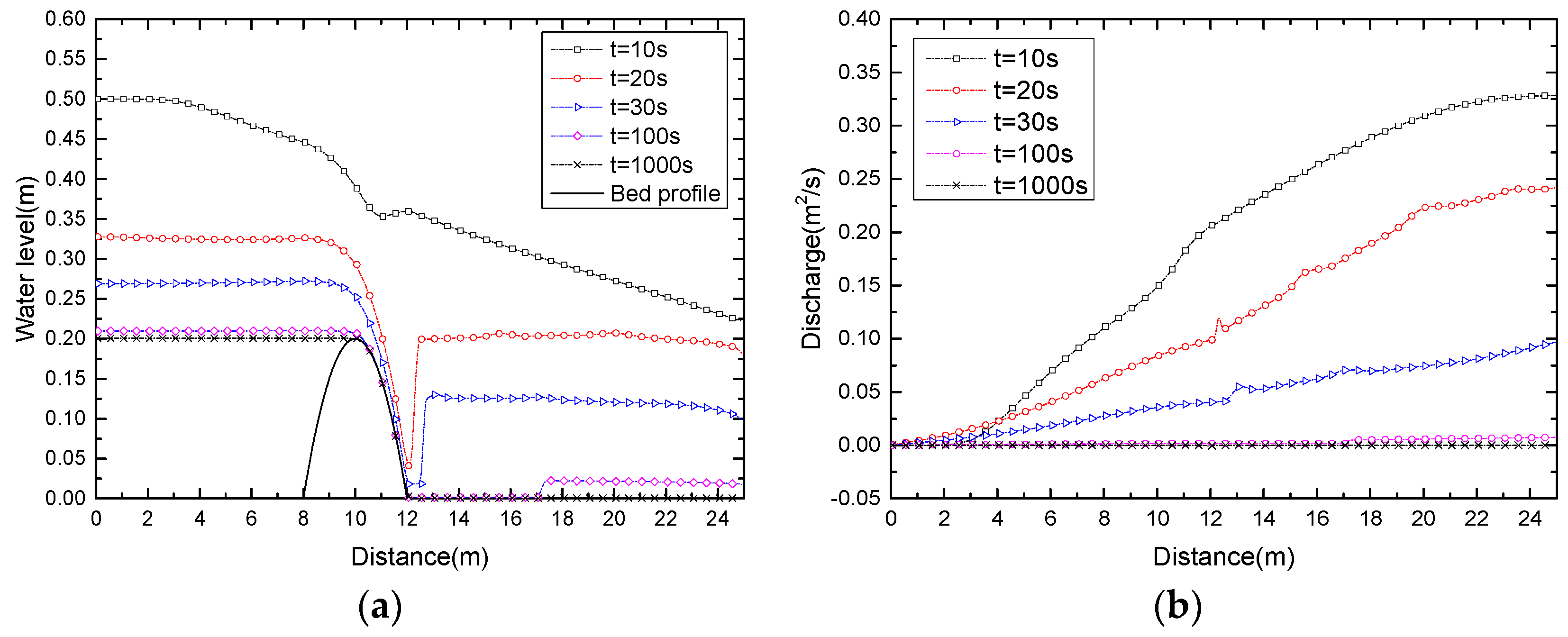
5.2. Drain on a Bump Bottom

In this test case, the bottom function is Equation (41) in Section 5.1 in the computational domain [0, 25]. The initial data are:

$$z(x,0)=h(x,0)+B(x)=0.5 \mathrm{m},\hspace{1em}hu(x,0)=0.0 {\mathrm{m}}^2/\mathrm{s}$$

(42)

The left boundary condition is a free condition on h and zero on hu. The right condition is a dry bed outlet [13,21]. A total of 250 uniform cells are used in the computational domain. The results at different times (t = 10 s, 20 s, 30 s, 100 s, 1000 s) are presented in Figure 12. Since a dry bed outlet is imposed on the right boundary condition, the water is freely flowing out of the domain on the right. At time t = +∞, the solution is a steady state, in which the water level z = h + B = 0.2 m and discharge q = 0.0 m²/s on the left of the top of the bump, and a dry zone (h = 0.0 m, q = 0.0 m²/s) on the right side of the bump. The numerical solutions converge to the expected steady state well.

Figure 12. Drain on a bump bottom at different times: (a) the water level; (b) the discharge.

5.3. Dam-Break Problem over a Plane

In this section, we consider a dam-break problem over a plane [13]. The computational domain is [−15, 15] and the bottom is given by

$$B(x)=1-x\tan (\alpha )$$

(43)

where the angle $\alpha$ will be defined as π/60 and −π/60 in this study. The initial condition is given by

$$\begin{array}{l}z(x,0)=h(x,0)+B(x)=\{\begin{array}{ll}1.0 \mathrm{m}& \mathrm{if} x<0\\ B(x)& \mathrm{otherwise}\end{array}\\ q(x,0)=hu(x,0)=0.0 {\mathrm{m}}^2/\mathrm{s}\end{array}$$

(44)

Concerning the boundary condition, the discharge q = 0 m²/s is imposed at x = −15 m, and a free boundary condition is considered at x = 15 m. In this numerical experiment, ∆x = 0.1 m.

The exact position of the wet/dry front is given by the following expression:

$$x_f(t)=2t\sqrt{g{h}_0\cos (\alpha )}-\frac{1}{2}g{t}^2\tan (\alpha )$$

(45)

where $\alpha$ is the angle in Equation (43) and h₀ = 1 m in this numerical experiment. Depending on different values of $\alpha$, various wet/dry fronts will appear. In this experiment, we consider two cases: $\alpha$ = π/60 and $\alpha$ = −π/60. Numerical results corresponding to the case $\alpha$ = π/60 (t = 0 s, 2.0 s, 2.5 s) are shown in Figure 13.

Figure 13. Dam-break problem over a plane for $\alpha$ = π/60: (a) the water level at t = 0.0 s, 2.0 s and 2.5 s; (b) comparison of the revised surface gradient method (RSGM) scheme and the present scheme at t = 2.0 s and 2.5 s near the wet/dry front.

The water level at times t = 0 s, 2.0 s and 2.5 s are shown in Figure 13a, and the comparison of the RSGM scheme and the present scheme at t = 2.0 s and 2.5 s near the wet/dry front is presented in Figure 13b. Observe in Figure 13b that the water level computed with the present scheme is tangent to the plane at the wet/dry front as was expected [22], and a small non-tangent front near the front appears with the RSGM scheme. The time evolution of wet/dry front location for $\alpha$ = π/60 and $\alpha$ = −π/60 are presented in Figure 14a,b, respectively. The analytical solutions are also shown in the figures for comparison. The conclusion can be drawn that the present scheme can predict the wet/dry front position well.

Figure 14. Dam-break problem over a plane. Time evolution of wet/dry position: (a) $\alpha$ = π/60; (b) $\alpha$ = −π/60.

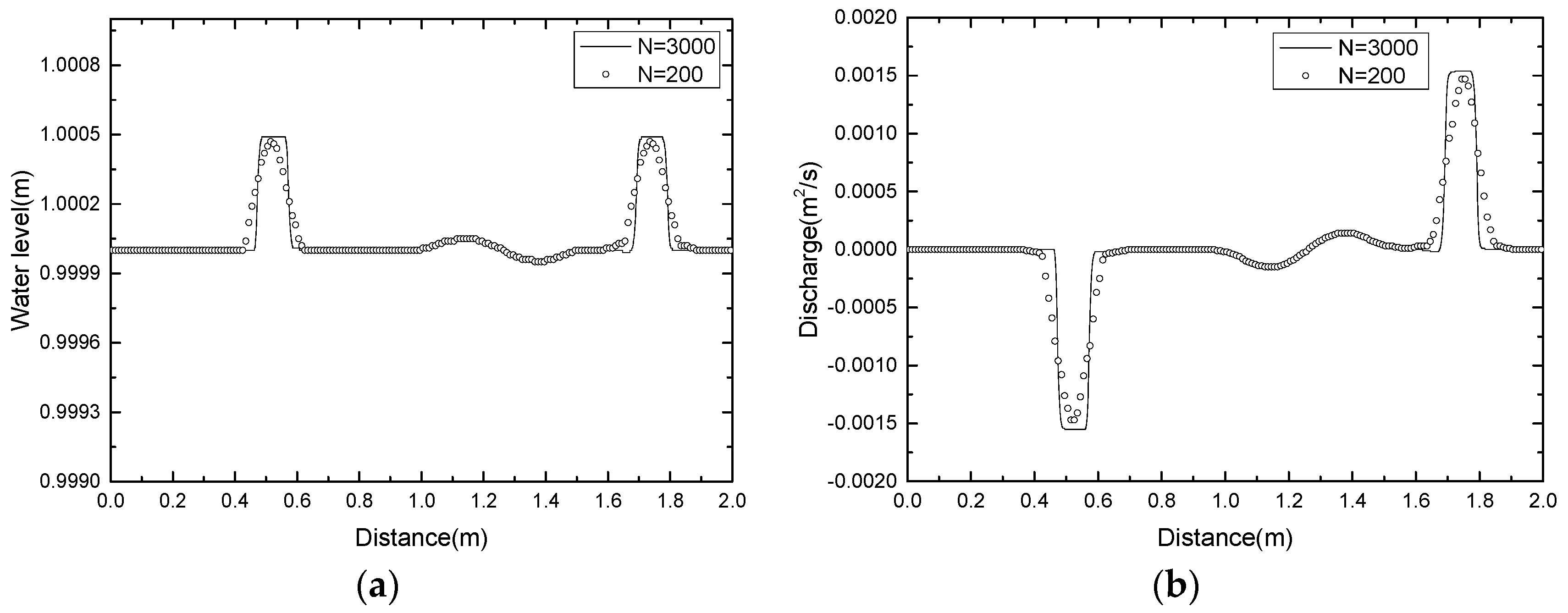
5.4. Small Perturbation Test

This numerical experiment was proposed by LeVeque (1998) and also tested by Xing, Y. et al. [23,24] to demonstrate the performance of our scheme on a rapidly varying flow over a smoothed bed. A stationary state is perturbed by a pulse. Theoretically, the pulse splits into two waves propagating in opposite directions, in which the left wave travels over a horizontal topography, and the right-going wave propagates over a bump.

The computational domain is [0, 2]. The bottom topography with one bump is given by

$$B(x)=\{\begin{array}{ll}0.25(\cos (10\pi (x-1.5))+1)& \mathrm{if} 1.4 \mathrm{m}\le x\le 1.6 \mathrm{m}\\ 0& \mathrm{otherwise}\end{array}$$

(46)

while the initial conditions are

$$q(x,0)=hu(x,0)=0.0 {\mathrm{m}}^2/\mathrm{s}, z(x,0)=h(x,0)+B(x)=\{\begin{array}{ll}1+\epsilon \mathrm{m}& \mathrm{if} 1.1 \mathrm{m}\le x\le 1.2 \mathrm{m}\\ 1 \mathrm{m}& \mathrm{otherwise}\end{array}$$

(47)

Here, $\epsilon$ is the height of perturbation constant. We take two cases: $\epsilon$ = 0.2 m (big pulse, see Figure 15), $\epsilon$ = 0.001 m (small pulse). The solution is taken at time t = 0.2 s with outflow boundary conditions and 200 cells. The results are shown in Figure 16 and Figure 17, for $\epsilon$ = 0.2 (big pulse) and $\epsilon$ = 0.001 (small pulse), respectively. We compare the solutions with that obtained with 3000 cells. The figures show that the numerical solutions have good performance on simulating the wave propagated by a big or small pulse over a smoothed bed.

Figure 15. Small perturbation test. The initial conditions with $\epsilon$ = 0.2 (big pulse).

Figure 16. Small perturbation test with $\epsilon$ = 0.2 (big pulse) and time t = 0.2 s: (a) the water level; (b) the discharge.

Figure 17. Small perturbation test with $\epsilon$ = 0.001 (small pulse) and time t = 0.2 s: (a) the water level; (b) the discharge.

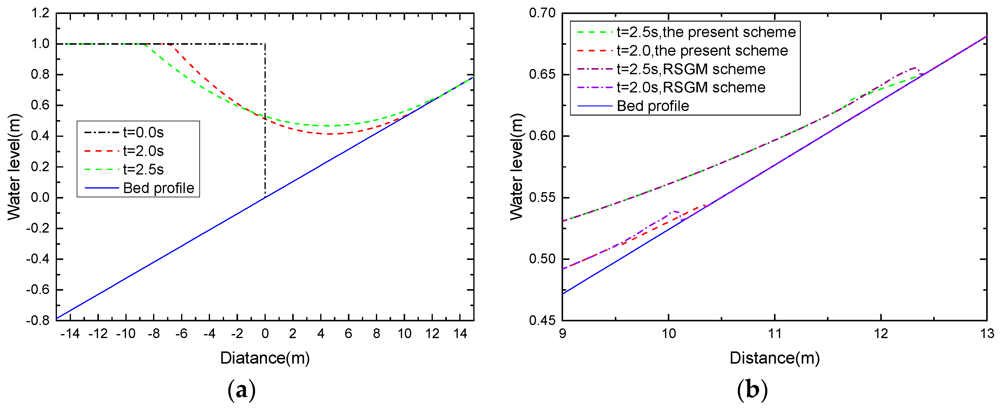
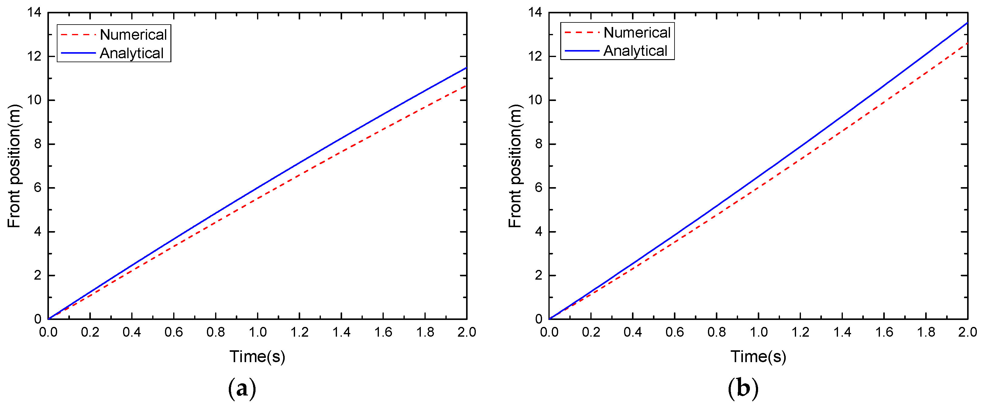
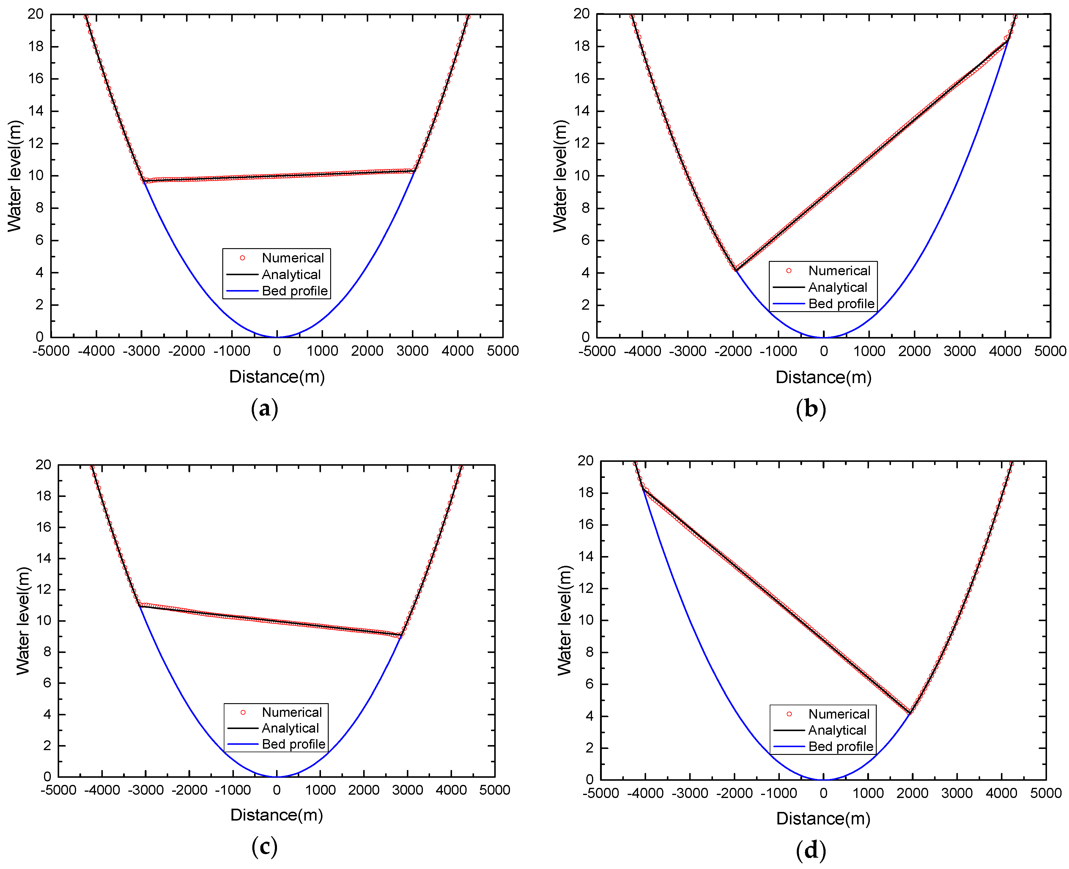
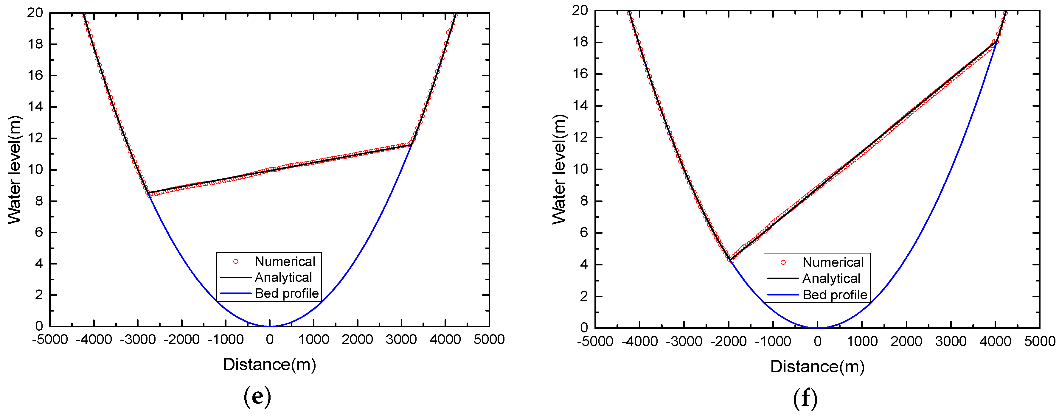
5.5. Evolution of Shorelines over a Parabolic Topography

Analytical solutions of one-dimensional shallow water equations were derived by Sampson et al. [25] for a perturbed flow with a parabolic topography. This provides a perfect test case for our scheme in dealing with the wet/dry front and bed slope. The parabolic bottom is defined by

$$B(x)=h_0{(x/a)}^2$$

(48)

with constant h₀ and a. The computational domain is [−5000 m, 5000 m] with 200 uniform cells. The analytical water level without the friction source term is given by

$$z(x,t)=h(x,t)+B(x)=\max (h_0-\frac{b^2}{4g}\cos (2\omega t)-\frac{b^2}{4g}-\frac{bx}{2a}\sqrt{\frac{8h_0}{g}}\cos (2\omega t),B(x))$$

(49)

where $\omega =\sqrt{2g{h}_0}/a$, and b is a given constant. The location of the wet/dry front is calculated by

$$x=-\frac{B\omega a^2}{2g{h}_0}\cos (\omega t)\pm a$$

(50)

The relevant coefficients are a = 3000, b = 5 and h₀ = 10 for the test case. The initial water level is defined by Equation (49) at time t = 0.0 and zero discharge. The boundary condition has no effect on the numerical solutions in this case as the flow cannot reach the boundaries. Figure 18 shows the numerical water level at different time (t = 1000 s, t = 2000 s, t = 3000 s, t = 4000 s, t = 5000 s, t = 6000 s,) with the comparison of analytical solutions, where a nice agreement is observed.

Figure 18. Wetting and drying over a parabolic topography; the water level at different times: (a) t = 1000 s; (b) t = 2000 s; (c) t = 3000 s; (d) t = 4000 s; (e) t = 5000 s; (f) t = 6000 s.

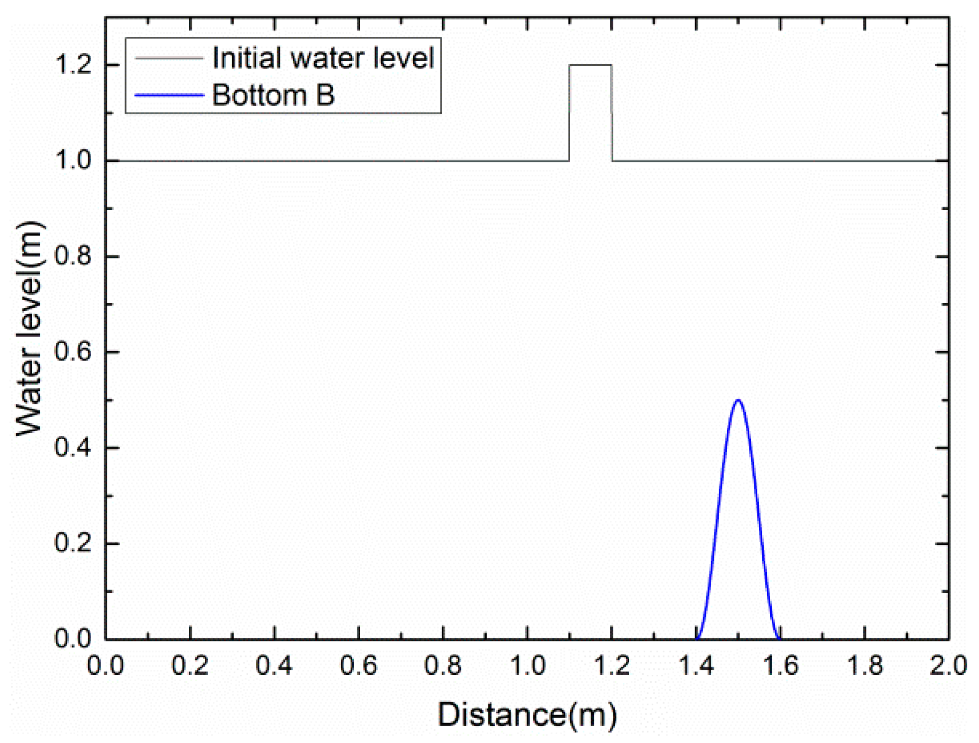
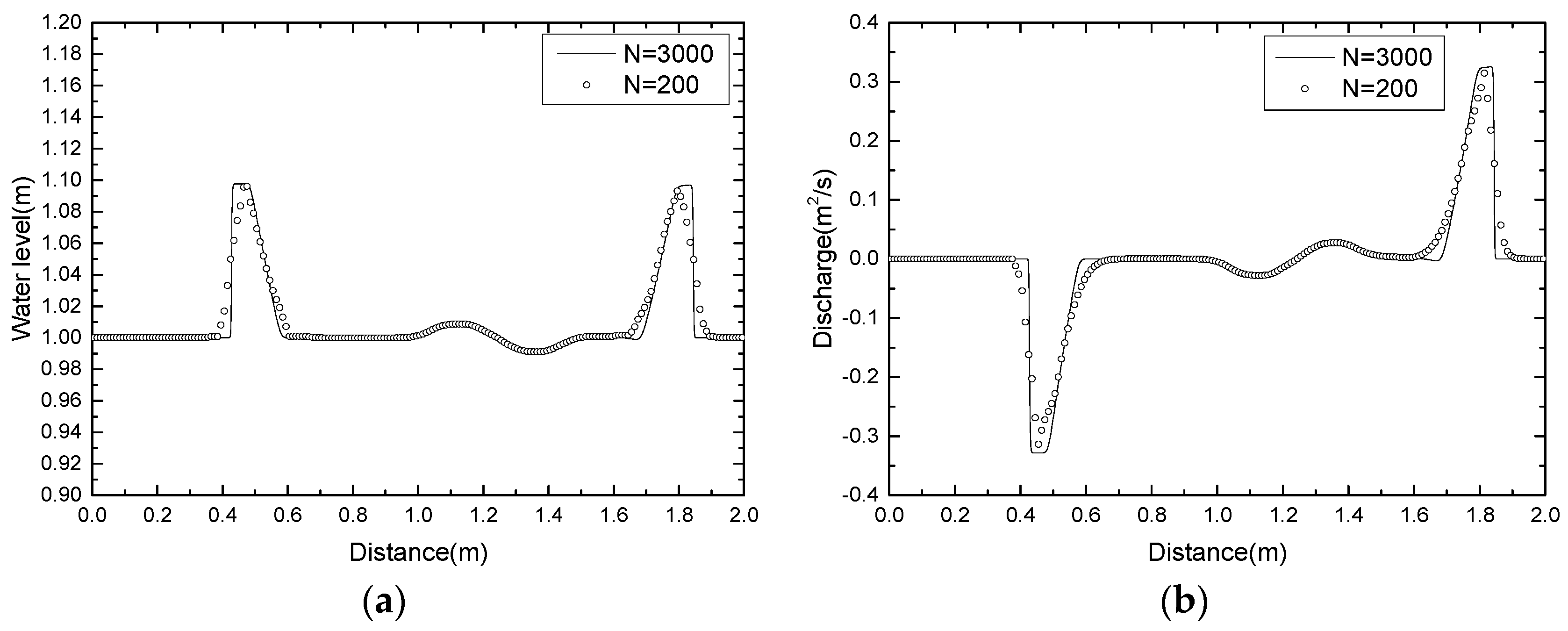
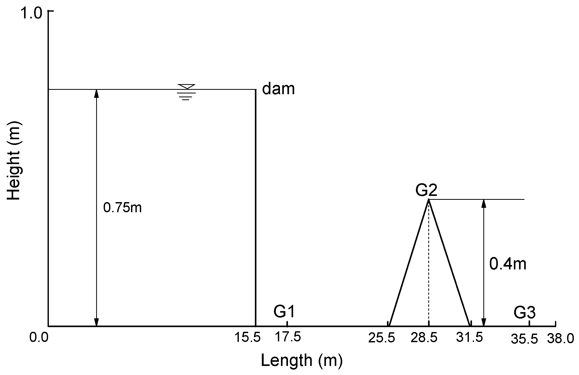
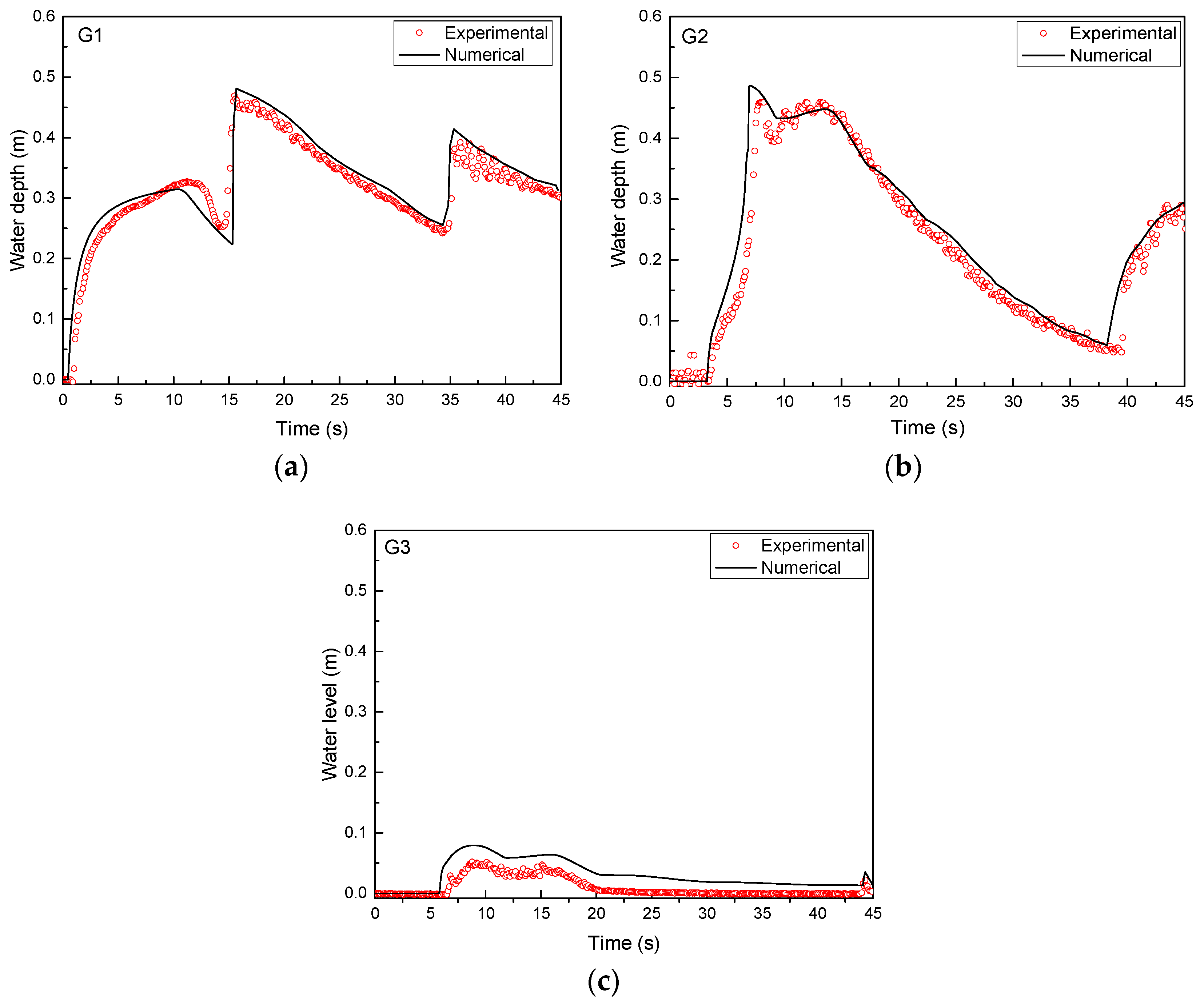
5.6. Experiments of Dam-Break over a Triangular Obstacle

A laboratory experiment of dam-break flow over a triangular obstacle was carried out by the EU Concerted Action on Dambreak Modelling (CADAM) project. In this test, the numerical results applied in the presented scheme are compared with the experimental measurements. Figure 19 shows the experimental set-up, in which the dam site is located 15.5 m downstream of the start of the domain (left boundary) and the domain has a length of 38 m. A triangular obstacle with height of 0.4 m and length of 6 m is located 25.5 m from the left boundary and 6.5 m from the right boundary.

Figure 19. Experimental set-up of a dam-break over a triangular obstacle.

The initial water depth is set to 0.75 m upstream of the dam with zero velocity and the rest of the domain is dry bed. A constant Manning coefficient n = 0.0125 is used throughout the domain. The upstream and downstream boundary conditions are assumed to be a solid wall and a free outlet, respectively. In the laboratory experiment, the dam suddenly fails and the water is released. The complex flow is associated with wave interactions, shocks, wetting and drying, and irregular bathymetry. Experimental and numerical time histories of the water depth at distances 17.5 m, 28.5 m and 35.5 m from the left boundary are plotted in Figure 20. It is concluded that the numerical results are satisfactory and the scheme can simulate complex flows with shock, irregular bathymetry and wetting/drying front.

Figure 20. Comparisons of numerical and experimental time histories at different gauges: (a) gauge 1 at 17.5 m; (b) gauge 2 at 28.5 m; (c) gauge 3 at 35.5 m.

6. Conclusions

In this paper, we present a new reconstruction technique including flooded cells and partially flooded cells that preserves the non-negative values of water depth at the cell interface. Two cases are considered: (1) If the cell is flooded, our proposed modified RSGM is applied assuming that the bed topography is irregular in the cell; and (2) if the cell is partially flooded, a special reconstruction of the flow variables is developed where the bottom function is assumed to be linear in the cell. The scheme is well balanced and preserves positivity for wet and dry cells.

References

- Bradford, S.F.; Sanders, B.F. Finite-volume model for shallow water flooding of arbitrary topography. J. Hydraul. Eng. 2002, 128, 289–298. [Google Scholar] [CrossRef]
- Hou, J.; Simons, F.; Liang, Q.; Hinkelmann, R. An improved hydrostatic reconstruction method for shallow water model. J. Hydraul. Res. 2014, 52, 432–439. [Google Scholar] [CrossRef]
- Liang, Q.H. Flood simulation using a well-balanced shallow flow model. J. Hydraul. Eng. 2010, 136, 669–675. [Google Scholar] [CrossRef]
- Wang, Y.L.; Liang, Q.H.; Kesserwani, G.; Hall, J.W. A 2D shallow flow model for practical dam-break simulations. J. Hydraul. Res. 2011, 49, 307–316. [Google Scholar] [CrossRef]
- Cunge, J.A.; Wegner, M. Intégration numérique des équations d’écoulement de Barré de Saint-Venant par un schéma implicite de différences finies. La Houille Blanche 1964, 1, 33–39. [Google Scholar] [CrossRef]
- Bollermann, A.; Chen, G.; Kurganov, A.; Noelle, S. A well-balanced reconstruction of wet/dry fronts for the shallow water equations. J. Sci. Comput. 2013, 56, 267–290. [Google Scholar] [CrossRef]
- Audusse, E.; Bouchut, F.; Bristeau, M.O.; Klein, R.; Perthame, B. A fast and stable well-balanced scheme with hydrostatic reconstruction for shallow water flows. SIAM J. Sci. Comput. 2004, 25, 2050–2065. [Google Scholar] [CrossRef]
- Liang, Q.H.; Marche, F. Numerical resolution of well-balanced shallow water equations with complex source terms. Adv. Water Resour. 2009, 32, 873–884. [Google Scholar] [CrossRef]
- Hubbard, M.E.; Garcia-Navarro, P. Flux difference splitting and the balancing of source terms and flux gradients. J. Comput. Phys. 2000, 165, 89–125. [Google Scholar] [CrossRef]
- Greenberg, J.M.; Leroux, A.Y. A well-balanced scheme for the numerical processing of source terms in hyperbolic equations. SIAM 1996, 33, 1–16. [Google Scholar] [CrossRef]
- Bermudez, A.; Ma, E.V. Upwind methods for hyperbolic conservation laws with source terms. Comput. Fluids 1994, 23, 1049–1071. [Google Scholar] [CrossRef]
- Gallardo, J.M.; Pares, C.; Castro, M. On a well-balanced high-order finite volume scheme for shallow water equations with topography and dry areas. J. Comput. Phys. 2007, 227, 574–601. [Google Scholar] [CrossRef]
- Xing, Y.L.; Zhang, X.X.; Shu, C.W. Positivity-preserving high order well-balanced discontinuous Galerkin methods for the shallow water equations. Adv. Water Resour. 2010, 33, 1476–1493. [Google Scholar] [CrossRef]
- Liang, Q.H.; Borthwick, A.G.L. Adaptive quadtree simulation of shallow flows with wet–dry fronts over complex topography. Comput. Fluids 2009, 38, 221–234. [Google Scholar] [CrossRef]
- Kurganov, A.; Petrova, G. A second-order well-balanced positivity preserving central-upwind scheme for the Saint-Venant system. Commun. Math. Sci. 2007, 5, 133–160. [Google Scholar] [CrossRef]
- Toro, E.F. Riemann Solvers and Numerical Methods for Fluid Dynamics; Springer: Berlin/Heidelberg, Germany, 1999; ISBN 978-3-662-03492-7. [Google Scholar]
- Zhou, J.G.; Causon, D.M.; Mingham, C.G.; Ingram, D.M. The surface gradient method for the treatment of source terms in the shallow-water equations. J. Comput. Phys. 2001, 168, 1–25. [Google Scholar] [CrossRef]
- Zhou, J.G.; Causon, D.M.; Ingram, D.M.; Mingham, C.G. Numerical solutions of the shallow water equations with discontinuous bed topography. Int. J. Numer. Meth. Fluids 2002, 38, 769–788. [Google Scholar] [CrossRef]
- Kim, D.H.; Cho, Y.S.; Kim, H.J. Well-balanced scheme between flux and source terms for computation of shallow-water equations over irregular bathymetry. J. Eng. Mech. 2008, 134, 277–290. [Google Scholar] [CrossRef]
- Toro, E.F. Shock Capturing Methods for Free-Surface Shallow Flows; John Wiley & Sons Inc.: New York, NY, USA, 2001; ISBN 0471987662. [Google Scholar]
- Gallouët, T.; Herard, J.M.; Seguin, N. Some approximate Godunov schemes to compute shallow-water equations with topography. Comput. Fluids 2003, 32, 479–513. [Google Scholar] [CrossRef]
- Peregrine, D.H.; Williams, S.M. Swash overtopping a truncated plane beach. J. Fluid Mech. 2001, 440, 391–399. [Google Scholar] [CrossRef]
- LeVeque, R.J. Balancing source terms and flux gradients in high-resolution Godunov methods: The quasi-steady wave-propagation algorithm. J. Comput. Phys. 1998, 146, 346–365. [Google Scholar] [CrossRef]
- Xing, Y.L.; Shu, C.W. High order finite difference WENO schemes with the exact conservation property for the shallow water equations. J. Comput. Phys. 2005, 208, 206–227. [Google Scholar] [CrossRef]
- Sampson, J.; Easton, A.; Singh, M. Moving boundary shallow water flow above parabolic bottom topography. Anziam J. 2006, 47, C373–C387. [Google Scholar] [CrossRef]
© 2018 by the authors. Licensee MDPI, Basel, Switzerland. This article is an open access article distributed under the terms and conditions of the Creative Commons Attribution (CC BY) license (http://creativecommons.org/licenses/by/4.0/).