Article

Multi-Model Approaches for Improving Seasonal Ensemble Streamflow Prediction Scheme with Various Statistical Post-Processing Techniques in the Canadian Prairie Region

1
Department of Civil Engineering, University of Manitoba, Winnipeg, MB R3T 5V6, Canada
2
Hydrologic Forecasting & Coordination, Manitoba Infrastructure, Winnipeg, MB R3C 0R8, Canada
3
Department of Civil Engineering, McMaster University, Hamilton, ON L8S 4L7, Canada
*
Author to whom correspondence should be addressed.
Water 2018, 10(11), 1604; https://doi.org/10.3390/w10111604
Submission received: 22 September 2018 / Revised: 5 November 2018 / Accepted: 5 November 2018 / Published: 8 November 2018
(This article belongs to the Section Hydrology)

Abstract

:
Hydrologic models are an approximation of reality, and thus, are not able to perfectly simulate observed streamflow because of various sources of uncertainty. On the other hand, skillful operational hydrologic forecasts are vital in water resources engineering and management for preparedness against flooding and extreme events. Multi-model techniques can be used to help represent and quantify various uncertainties in forecasting. In this paper, we assess the performance of a Multi-model Seasonal Ensemble Streamflow Prediction (MSESP) scheme coupled with statistical post-processing techniques to issue operational uncertainty for the Manitoba Hydrologic Forecasting Centre (HFC). The Ensemble Streamflow Predictions (ESPs) from WATFLOOD and SWAT hydrologic models were used along with four statistical post-processing techniques: Linear Regression (LR), Quantile Mapping (QM), Quantile Model Averaging (QMA), and Bayesian Model Averaging (BMA)]. The quality of MSESP was investigated from April to July with a lead time of three months for the Upper Assiniboine River Basin (UARB) at Kamsack, Canada. While multi-model ESPs coupled with post-processing techniques improve predictability (in general), results suggest that additional avenues for improving the skill and value of seasonal streamflow prediction. Next steps towards an operational ESP system include adding more operationally used models, improving models calibration methods to reduce model bias, increasing ESP sample size, and testing ESP schemes at multiple lead times, which, once developed, will not only help HFCs in Canada but would also help Centers South of the Border.

1. Introduction

The science of hydrological forecasting has greatly improved with the introduction of numerous distributed hydrologic models, numerical weather models (NWMs), and data assimilation techniques [1]. A large number of hydrological forecasting models are in operation around the globe, and several of these are used in Canada [2]. However, no single hydrologic model is suitable for all drainage systems due to the varying characteristics and complexities of watersheds, local-scale heterogeneity, and different climate zones [3]. The model used by a forecasting unit is dependent upon the data availability, hydrologic expertise, type of the watershed, and the specific nature of the problem. Distributed and physically based hydrologic models are data-intensive but are considered to be reliable in providing improved streamflow forecasting, mainly because they are capable of leveraging a variety of spatially distributed data [4,5]. In operational forecasting, however, there are trade-offs between the complexity of the model, the inclusion and accuracy of catchment-scale processes affecting runoff generation, and the model speed. The goal is always, and always must be, the highest accuracy forecasts for reliable, operational flood management and warning [6,7].
Flood forecasting is not only required to be sufficiently accurate within a defined time horizon but must also provide information on the forecasting uncertainty to facilitate effective decision-making and the timely issuing of forecasts [8]. Consideration of uncertainty has been recognized as an essential component for both research and operations [9,10], and provides added value in water-resources-related decision-making. Informed uncertainty prediction can increase confidence in forecasts, which are most certainly imperfect [11]. Four major sources of uncertainty have been identified: input, parameter, model structure and uncertainty due to observations, or output uncertainty [10,12]. Several approaches have been developed to assess uncertainty in hydrological modeling [13,14]. Among others, the ensemble streamflow prediction (ESP) [15] approach has led to the development of Hydrological Ensemble Prediction System (HEPS) [16,17] which allow us to estimate uncertainty in weather forecasts as well as predicting the most likely outcomes [18].
In ESP, hydrologic models are forced with historical sequence of climate data, such as precipitation, temperature and/or potential evapotranspiration during the time of forecast, providing a plausible range of future streamflow states [19]. The method assumes that the forcing data and model are perfect, that is, there are no errors in the initial hydrological conditions (IHCs) [20]. In operational practice, the skill attributed to IHCs has been ranked high in comparison to the skills attributed to the climate forecast [21], with both being the two major contributing factors to successfully predicting streamflow dynamics.
Whether or not forecasts are generated using deterministic or ensemble methods, raw forecasts should not be used directly for operational decision-making due to their bias [22]. Consequently, a number of hydrological post-processing statistical techniques [23,24] have been developed to improve the ability of a forecast which accounts for uncertainty in the hydrological output. This has led to the development of schemes that seek to obtain consensus from a combination of multiple model predictions to compensate for errors in one model by the others.
This study is designed to develop a new post-processing tool to help identify the uncertainty in seasonal streamflow forecasts for the Manitoba Hydrologic Forecast Centre (HFC) using their operational forecasting model (WATFLOOD), and one newly developed research-based model (SWAT). The goal is to improve ensemble decision-making capacity for the Manitoba HFC by 1) developing a framework to evaluate the forecast skill of an ensemble of hydrologic models, and 2) developing a tool to explore the use of four post-processing approaches for ensemble forecasting: Linear Regression (LR), Quantile Mapping (QM), Quantile Model Averaging (QMA), and Bayesian Model Averaging (BMA). Through the study, it is intended to answers these questions: What ensemble-generating mechanism results in a better forecast? Moreover, how can post-processing schemes be used to improve the reliability and accuracy of forecasts?
Although, ESP with post-processing techniques have been tested widely around the globe, the novelty of this research lies in the methodological choices of testing different combinations of ESP and statistical post-processing schemes. We further aim that this study is the first of its kind that utilizes more than two semi-physically based distributed models with multiple post-processing techniques in the Prairie Pothole Region, known for its complex hydrological landscape. This study falls under Theme 3 of the Canadian Natural Science Engineering Research Centre (NSERC)-funded FloodNet project that aims to enhance flood forecasting systems across Canada [25].

2. Materials and Methods

2.1. Study Area

The study area selected for this study is the Upper Assiniboine River basin (UARB) at Kamsack, Canada. The UARB at Kamsack is characterized by the presence of potholes that creates intermittent flow, the existence of numerous lakes, and the dynamics of the wetlands. Located at the border of Saskatchewan and Manitoba, the UARB at Kamsack has a total area of 13,000 km2 and is monitored by five streamflow gauging stations (Figure 1). The basin is of significant importance as flow generated in the basin enters the Lake of the Prairies (Shellmouth Reservoir), which was constructed as a multipurpose water control structure and is located approximately 45 km downstream of the watershed outlet.
The climate of the UARB is continental sub-humid characterized by long, cold winter and short summer seasons where the mean annual temperature and potential evapotranspiration are about 1 °C and 850 mm, respectively [26]. The average annual precipitation is 450 mm, with approximately 26% of the precipitation falling as snow [27]. Spring freshet occurs from April to June, accounting for 82%, on average, of total mean annual streamflow volume [27] (Figure 2).

2.2. Hydrological Model

This study utilized two hydrological models to generate ESPs. The WATFLOOD model, a semi-physically based distributed model; and SWAT, a physically based, semi-distributed hydrologic model. The WATFLOOD model is currently used as an operational forecasting tool for reservoir inflow forecasting at the Manitoba HFC while the SWAT model has been developed as a research tool at the University of Manitoba. A brief overview of each model including its calibration protocol is presented in subsequent sections. To provide accurate feedback to the HFC on the current state of their operational models, we purposely did not re-calibrate the operationally used model (WATFLOOD), utilizing in-house model setup and calibration.

2.2.1. WATFLOOD Model

WATFLOOD is a partially physically based and fully distributed hydrological model that is used in operation at the Manitoba HFC for flood forecasting. The model uses conceptualization of some physical processes in order to maintain high computational efficiencies [28] and operates on a grouped response units (GRUs), which are hydrologic computational units that are expected to respond similarly to meteorological conditions [29,30]. Groups are formed based on hydrological similarity generally defined by land cover types. WATFLOOD relies on the assumption that similar land covers exist in regions of similar soil types and topographic conditions. Response in each GRU of a grid is summed to give a total hydrologic response to the grid. The grids combine together to form the watershed basin where the upstream gridded responses are routed to downstream grids.

2.2.2. SWAT Model

The SWAT model is a continuous-time, processes-based, semi-distributed watershed-scale model that can be employed to assess the effect of land management practices on water resources in large river basins [31,32]. The hydrology, erosion, weather, plant growth, nutrients, pesticides, land management, channel, and reservoir routing are the major hydrological component of the SWAT model.
A watershed in SWAT is first divided spatially into subbasins, which are further subdivided hydrological response units (HRUs). HRUs in SWAT are the smallest computational unit, consisting of land use, digital elevation model (DEM), and soil map of the area, having similar landscape characteristics. A daily hydrological balance for each HRU is simulated that includes partitioning of precipitation, snowmelt water, redistribution of water within the soil profile, evapotranspiration and return flow [32,33]. Streamflow in SWAT is simulated as the combined runoff from all HRUs in the subwatershed routed through the stream network using either the variable rate storage method [34] or the Muskingum method [32].
In this study, a modified version of the SWAT model was used that has enhanced representation of pothole wetlands [35,36] which are unique to the Prairie Pothole Region. The reader is referred to [35] for more detail on the modified concept of pothole wetlands representation in SWAT.

2.3. Statistical Post-Processing

A straightforward method of statistical post-processing of model output is the arithmetic mean, also known as simple model averaging (SMA). It is based on the assumption that all ensemble members have equal likelihood of occurrence, and that the ensemble size is irrelevant. That is, the MM hydrologic predictions are formed by merging the individual runoff forecasts with equal weightings [37]. Although the method has been shown to be more reliable than deterministic model predictions in some cases [38,39], studies suggest that SMA does not make full use of all the information available to the ensemble members [40]. This is mainly because the SMA treats the good and bad simulations equally, thus yielding an intermediate solution. Consequently, the SMA does not guarantee an improved estimate, and in some cases, estimates may even be worse than individual model simulations. Techniques such as LR [41], BMA [42], and QMA [43] are developed to overcome the limitations of SMA.
We present a brief overview of the statistical post-processing techniques used in this study; the reader is referred to [44] for further detail. The LR method developed by [41] uses the mean of ESP with observations to generate the conditional forecast mean and spread to improve upon the traditional ESP forecast. The method, however, may not be of great help during extreme events such as flood warnings, as parameters are trained using the mean rather than the extreme, due to the rarity of the extreme events. The QM method adjusts the cumulative distribution function (CDF) of the forecast according to the CDF of the observations, thus mapping the forecast value to the corresponding quantile in the observed CDF [41,45]. A noted weakness of the method is that it does not preserve the connection between each pair of forecast and observations value, leading to unsatisfactory results [22]. Furthermore, the LR and QM are mostly applied in cases when ESP is generated using single hydrological models. Consequently, post-processing techniques, such as BMA and QMA, are developed to overcome this limitation and to merge ESPs from multiple hydrologic models, while appreciating individual model performance. The BMA method [42] is one of the most popular MM post-processing methods, where each member of the ensemble forecast is associated with a conditional probability distribution function (PDF). A weight for each member of the ensemble forecast is computed based on the performance of the model during the training period, such that all weights sum to 1. QMA, on the other hand, is the weighted average of forecast quantiles from all the models [43]. A noted difference between BMA and QMA is that BMA produces bimodal outputs while QMA produces smooth and unimodal distributions [43]. All mentioned post-processing techniques have been extensively used to reduce uncertainty in hydrologic predictions that arise from different sources, including atmospheric forcing and prediction, model initial states, model parameters, model structure, and assumptions, among others [20,46,47].

2.4. Forecast Generation

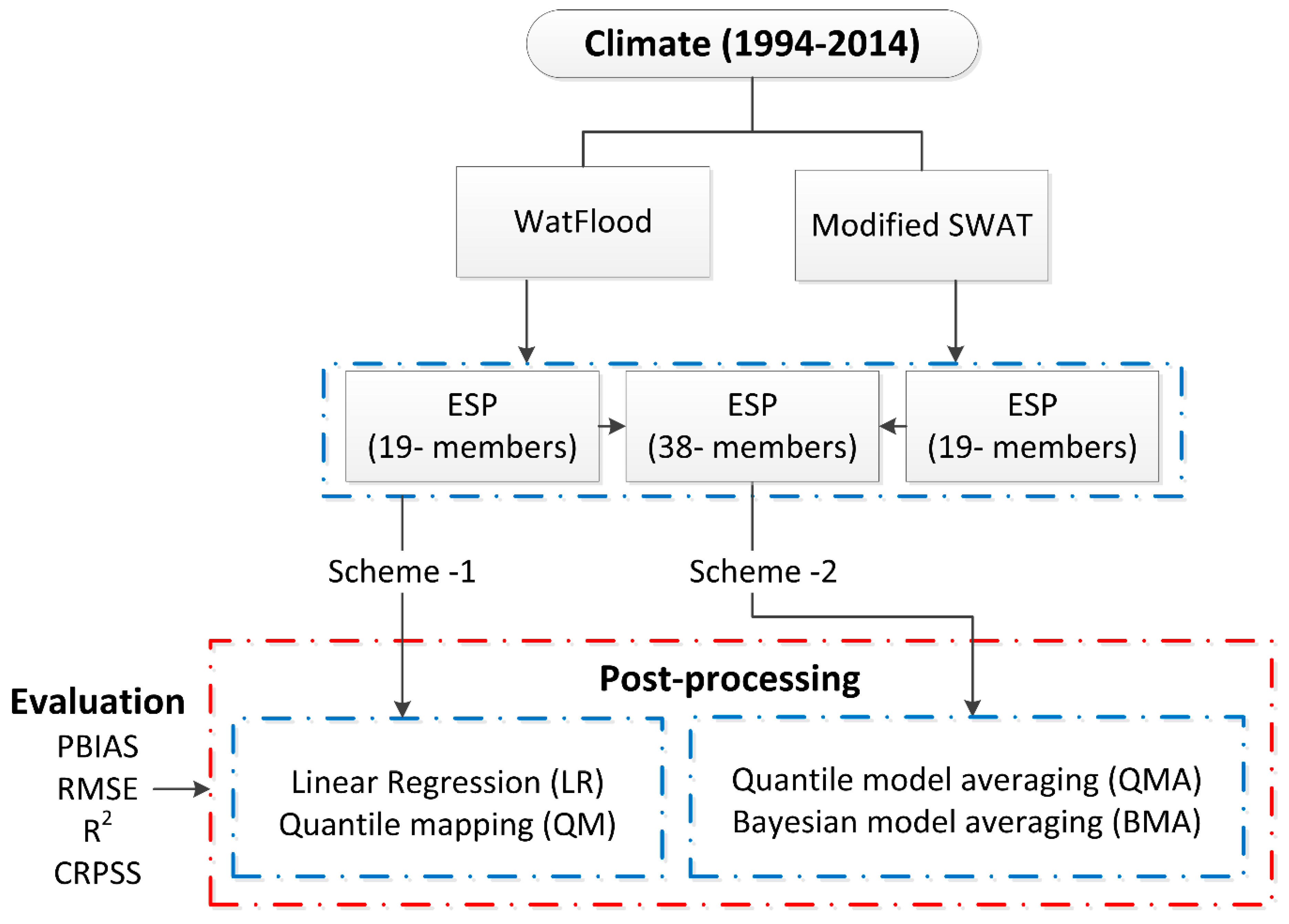
We utilized historical observations from 1994 to 2014 to generate probabilistic (ensemble) streamflow hindcasts, using 1994 as a spin-up period. Each model was repeatedly forced with the observed meteorological input of Environment and Climate Change Canada (ECCC) gauging stations up until the time of the hindcast initialization, leading to a sample size of 20 (i.e., one hydrologic sequence per year used for 20 years, based on previous meteorological conditions). Following the Manitoba HFCs methodology, the year of interest (i.e., hindcast year) was withdrawn during ESP generation; thus, the total number of ensemble members generated for the ESP (per hydrologic model) was 19. In Manitoba, spring streamflow outlooks are issued twice a year: at the end of February and at the end of March while runoff conditions are monitored throughout the year. The most important runoff period for the UARB is April–July, which generates more than 80% of annual streamflow volume [27]. The study thus focused on April-to-July runoff volume. A schematic outlining the procedure we used to generate the ensembles is presented in Figure 3. Scheme-1 results in 19 ensembles per model, while Scheme-2 combines all ensemble members (regardless of the model used to generate it), resulting in 38 members. Hindcasts for each scheme were issued and were then post-processed using the LR, QM, BMA, and QMA techniques.

2.5. Performance Metrics

To evaluate the quality of the hindcasts, percent bias (PBIAS), Root Mean Square Error (RMSE), Coefficient of determination (R2), and the Continuous Ranked Probability Skill Score (CRPSS) were used. The percent bias computes the average tendency of the simulated variable to be larger or smaller than the observed variable and can be expressed using Equation (1):
P B I A S = 100 × 1 n ( Q o   Q s ) i 1 n Q o
where Q is a variable (e.g., discharge), and o and s stand for the observed and simulated variable, respectively. The optimum value is 0; however, values between –25 and 25 are considered satisfactory [48]. Values above zero mean the model is underpredicting, while PBIAS below 0 indicates the models are overpredicting.
RMSE measures the difference between observed and simulated values. Individual differences are also called residuals, and the RMSE serves to aggregate them into a single measure of predictive power. The RMSE is expressed in Equation (2):
RMSE = 1 n ( Q o   Q s ) 2 i n
The threshold for RMSE is difficult to establish; however, RMSEs of >0.5 are often related to a model with decreasing predictive power [49].
The R2 is an index that measures the degree of linear relationship between observed and simulated values and can be computed using Equation (3):
R 2 =   1 n [ ( Q o   Q ¯ o ) × ( Q s   Q ¯ s ) ] 2 1 n ( Q o   Q ¯ 0 ) 2 × ( Q s   Q ¯ s ) 2
where bars represent average variables over a given time period. R2 ranges between −1 and 1, with 1 being perfectly positive and −1 as the perfectly negative relationship. When R2 is 0, it implies that there is no connection between observed and simulated variables.
The CRPSS (Equation (4)) is a widely utilized performance metric that assesses the overall quality of the probabilistic forecast (or hindcast) in reference to the climatology-based ensemble, which, in most cases, is the reference forecast (or hindcast) [50,51]:
CRPSS = 1 CRPS ¯ CRPS ¯ ref
where
CRPS = [ F ( y ) F 0 ( y ) ] 2 dy
and
F 0 ( y ) = { 0 , y   < Observed   value 1 , y   Observed   value
F(y) is a stepwise CDF of the ESP for each considered forecast (hindcast). CRPSS ranges from –∞ to 1, where 1 indicates a perfect forecast (hindcast), and positive values indicate high skill over the reference period.

3. Results and Discussion

3.1. Hydrologic Model Evaluation

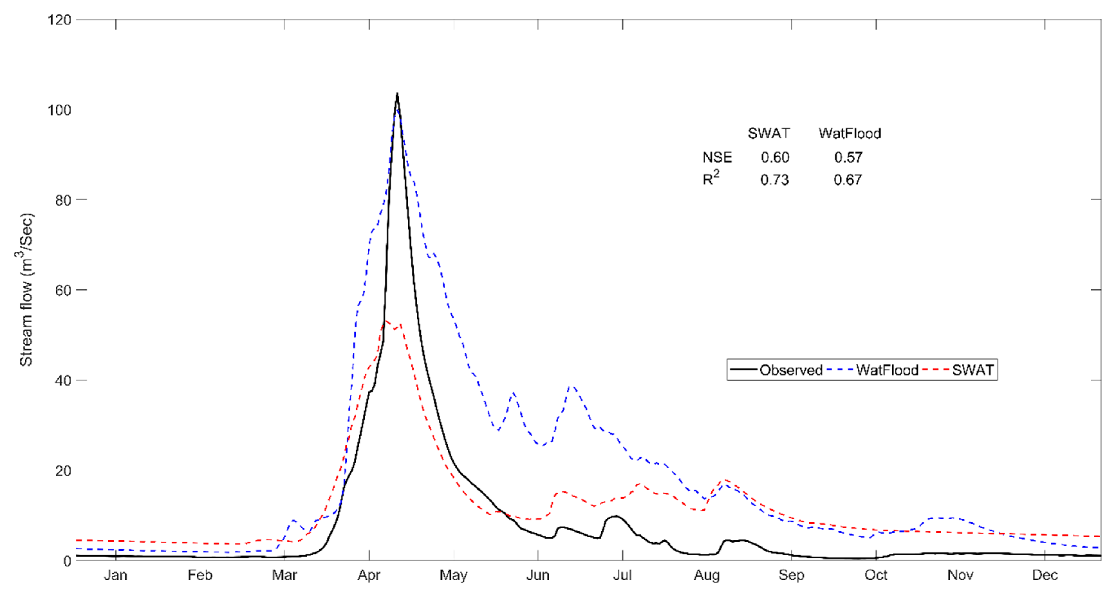
Daily average annual hydrographs using two hydrologic models (WATFLOOD and SWAT) were hindcast from 1994 to 2004 and compared to observed streamflow (Figure 4). In general, both hydrologic models followed the trend of observed streamflow and were able to capture the timing of the spring runoff; however, there are inconsistencies in capturing the correct magnitude of runoff for both models. This could be a result of the model’s individual calibrations, but can also, in part, be explained by the developed philosophy behind each model. For example, SWAT is an agricultural model, which is developed to most accurately predict the impacts of best management practices (BMPs) on water, sediments, and nutrient loading across large spatial scales and over long periods of time. This results in SWAT being able to provide reasonable simulations of long-term, average-to-low-flow conditions for the watershed (Figure 4). Whereas WATFLOOD was developed for operational flood forecasting in an agriculturally dominated landscape [52], where physically based routing assists the model in predicting peak flows more accurately. Furthermore, wetlands play an important role in correctly attenuating streamflow in the UARB, as do the dynamic contributing areas which are internally drained and only contribute to streamflow after reaching their maximum storage capacity [53]. Structurally, the two models differ substantially in how they simulate these crucial hydrological storages and dynamic connectivity within the channel network. The version of SWAT used in this study [35] has an enhanced spatial representation of the Prairie Pothole wetlands that is dynamic and modifies the wetland-channel routing network. In WATFLOOD, the wetland area is defined using a (constant) threshold value that splits wetlands into coupled wetland-channel region (i.e., riparian areas) and uncoupled (disconnected from the channel) regions. While uncoupled wetland area does not contribute to channel flow, the coupled wetlands have a dynamic interaction with the channel based on the Dupis–Forecheimer formulation (Kouwen, 2018). This wetland routing scheme is robust and computationally efficient; however, it does not recognize the dynamic spatial relationship between isolated wetlands and the channel that is determined by annual antecedent conditions. Results are similar to those found in [54], where models are criticized for their inconsistency in correctly capturing the magnitude of runoff in the UARB due to their structural differences. We further assessed the performance of the models using the Nash–Sutcliffe model efficiency coefficients (NSEs) and R2 for WATFLOOD (0.57, and 0.67, respectively) and SWAT (0.60, and 0.73, respectively). As per [49,55,56], both models performed satisfactorily in this study based on NSE values of >0.5 and R2 of >0.5.

3.2. Deterministic Evaluation of the Benchmark and Post-Processed ESPs

The two schemes proposed for assessing the various post-processing approaches (Figure 3) were compared to the observed April-to-July runoff period using the mean volume at the outlet of the UARB at Kamsack (WSC ID: 045MD004). The flow generated in the UARB at Kamsack enters Lake of the Prairies (the Shellmouth Reservoir), which was solely constructed to regulate flow and mitigate floods. Thus, it is of critical importance to determine the volume of inflow generated in the upstream basin for reservoir optimization and flood forecasting operations. The LR and QM post-processing techniques are applicable when ensembles are generated from a single model. Both techniques can also be applied when a multi-model (MM) ensemble is placed together to increase ensemble size (i.e., considering the ensembles of the two hydrologic models as a single forecast product), whereas QMA and BMA techniques are applicable when weights are used for each model based on their relative performance.
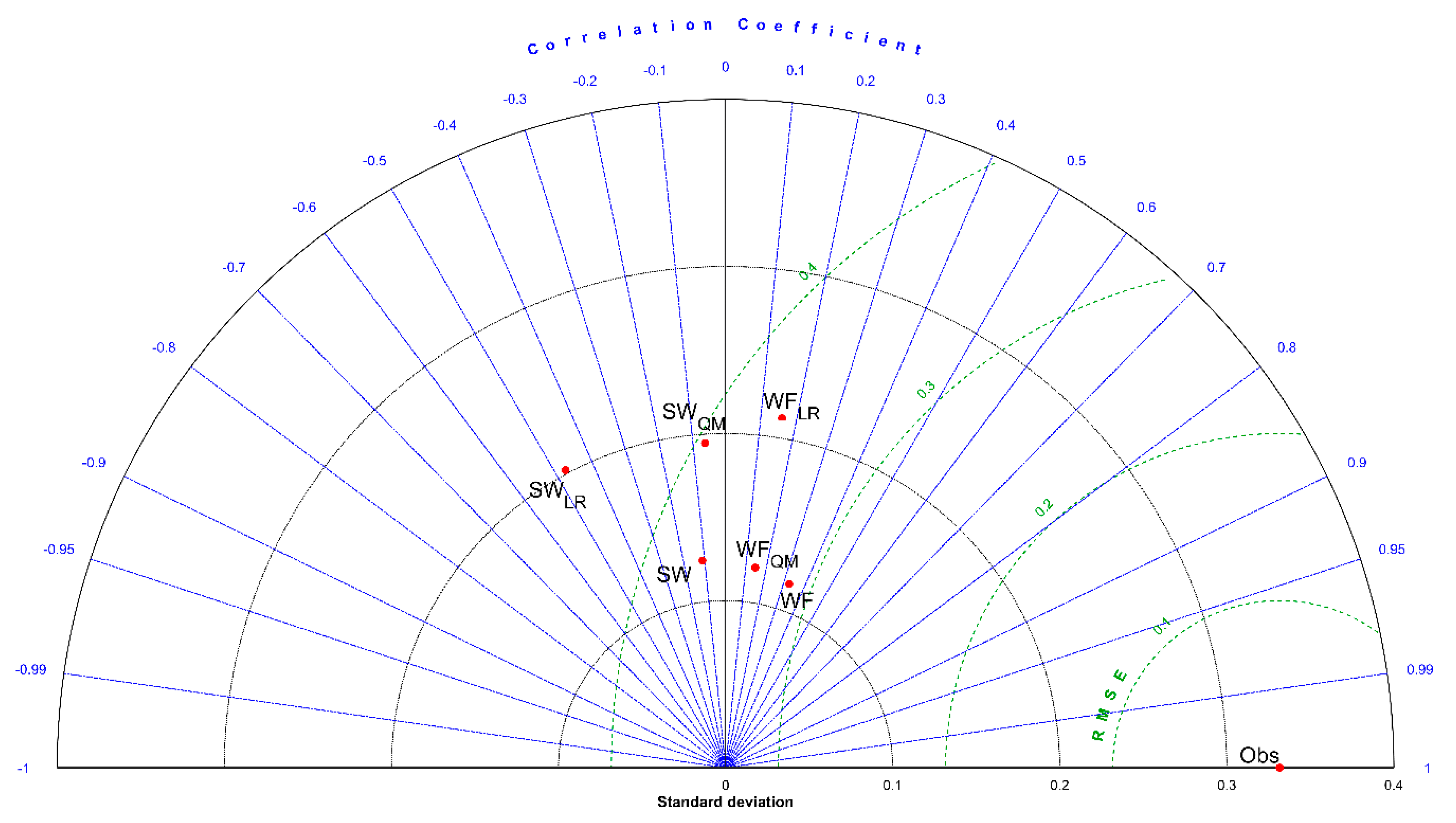
In our experiment, Scheme-1 represented the application of LR and QM post-processing techniques on the ensemble of each of hydrological model (Figure 5), while in Scheme-2, all post-processing techniques were applied to the MM ensemble (Figure 6). WATFLOOD indicated better correlation (R2 closer to 1) and lower RMSE relative to the observed streamflow in comparison to SWAT (Figure 5). SWAT, however, reflected a lower standard deviation dispersion, indicating it more often captured the mean simulations. Post-processing the ensembles in Scheme-1 does not appear to improve the predictability of observed streamflow for both hydrologic models, and it appears that the benchmark ensemble (raw ESPs) in fact provides the best hindcast (Figure 5).
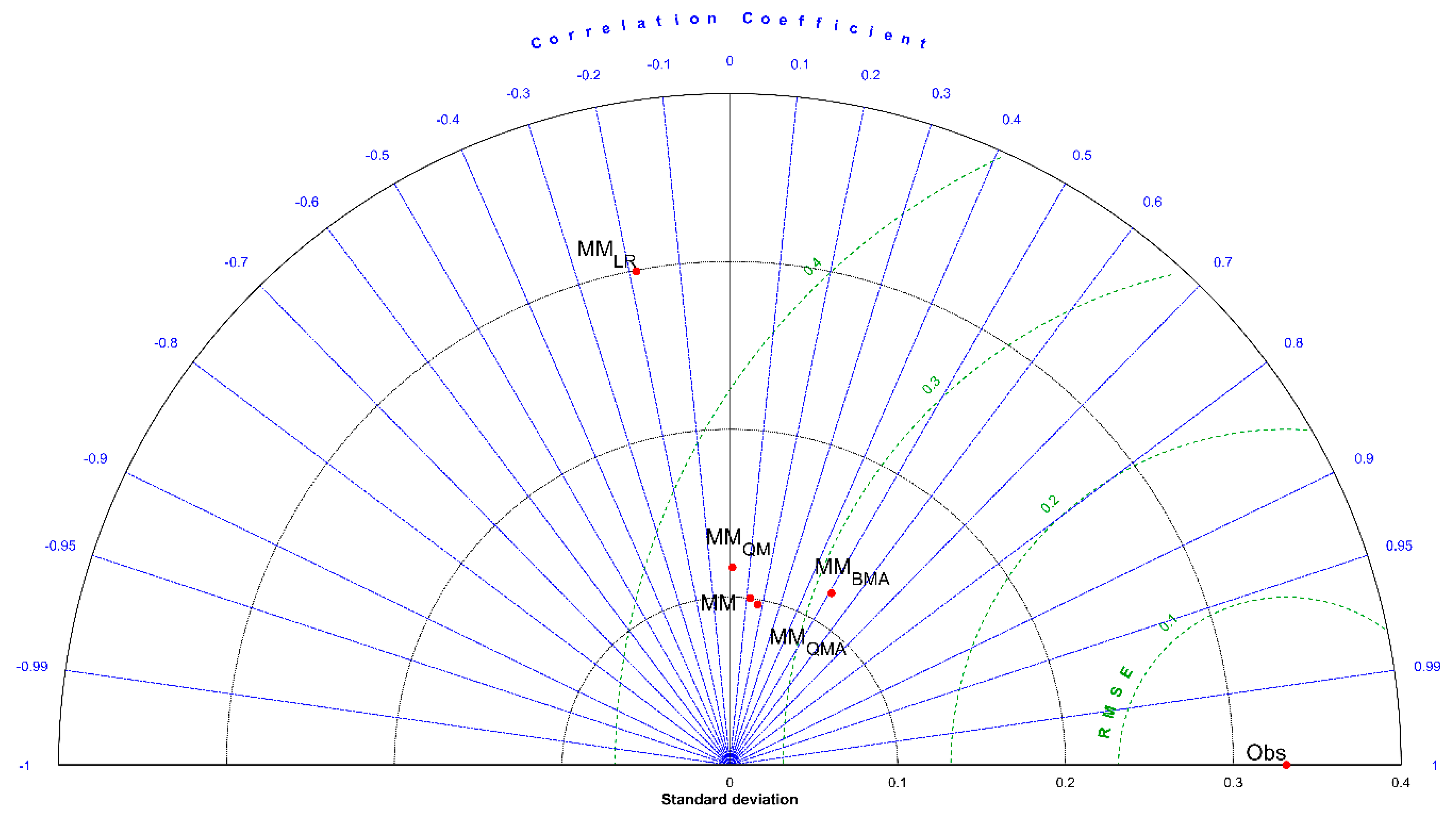
Scheme-2 combines the two hydrologic models and evaluates the LR, QM, BMA, and QMA post-processing techniques (Figure 6). Both BMA and QMA improved the predictability of observed streamflow volume the most, given their improved correlation (positive R2) and lower RMSE in comparison to the benchmark MM ensemble. Linear Regression (LR) and Quantile Mapping (QM) techniques have lower correlation and higher RMSE, in comparison. There are a number of reasons why the application of various post-processing techniques did not more significantly improve the predictability of seasonal runoff volume. For seasonal lead times (as opposed to hourly or daily), the accurate determination of IHCs is of critical importance and would exert a dominant influence on the hydrologic forecast [55,56,57]. The Prairie Pothole Region is a hydrologically diverse and complex landscape that makes accurately defining the IHCs prior to the time of hindcast difficult at best. Post-processing would be expected to have a more pronounced impact (on improving predictability) if IHCs during the time of the hindcast were sufficiently represented [44].
Furthermore, the suitability of post-processing techniques is highly dependent on the sufficiency of a hindcast time series, and consistency of retrospective model runs, used to train the post-processing methods [20,58]. In a study by [21] a sample size of 23 ESP members are used to train the model. However, another recent study by [44] outlined that three years of daily short-range forecasts would provide a nominal sample size of over 1000 records for training the post-processing method parameters to account for different hydrologic regimes. A 30-year hindcast for seasonal prediction offers a sample size of 30 members, thus making it difficult to estimate the optimum parameter value in a statistical post-processing model. It is likely that the low impact of the various post-processing approaches tested on the seasonal runoff hindcast resulted from the limited sample size used in this study.

3.3. Probabilistic Evaluation of the Benchmark and Post-Processed ESPs

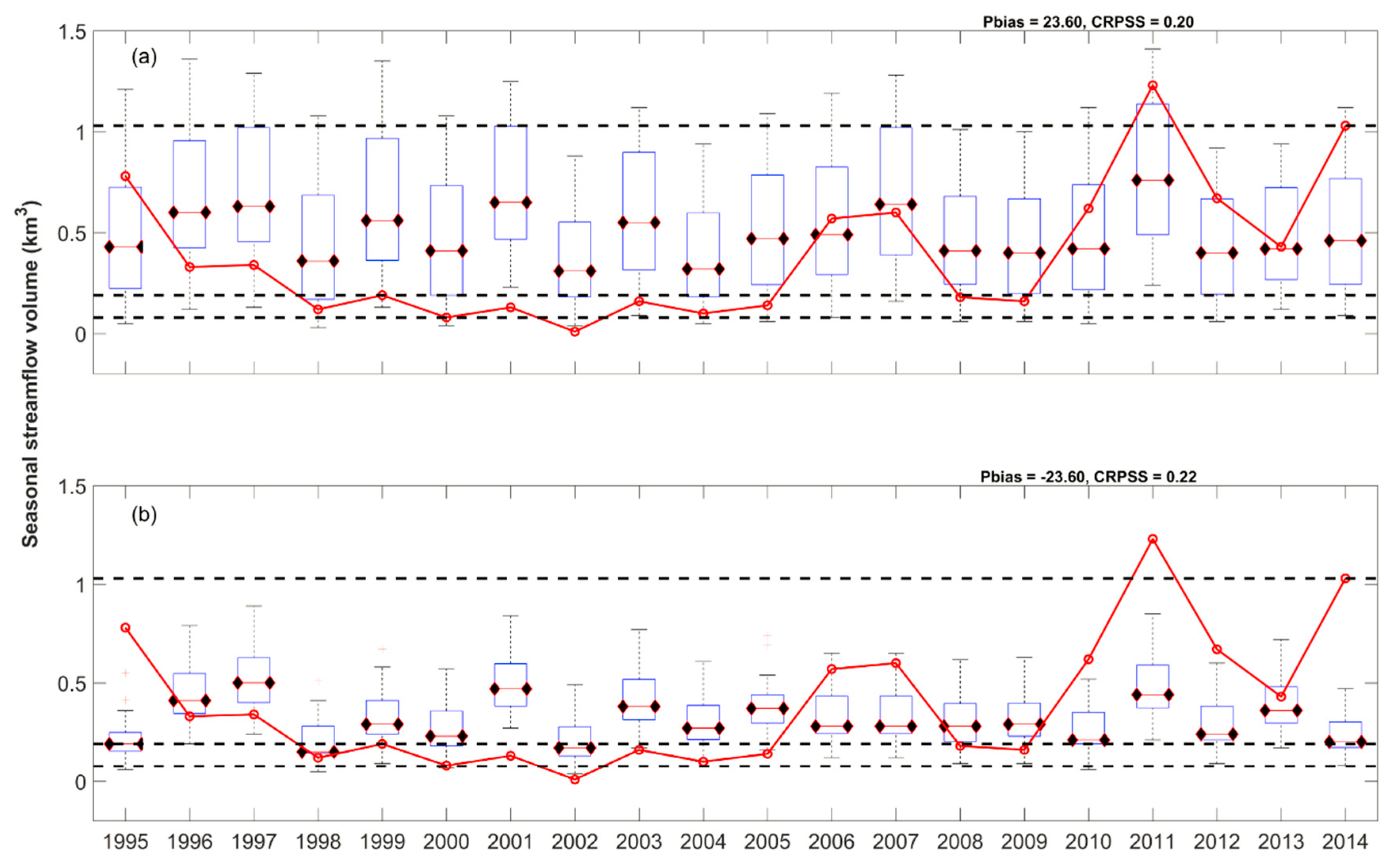
The benchmark ESPs from both the WATFLOOD and SWAT hydrologic models are presented in Figure 7. The benchmark ESP from WATFLOOD appears to better capture peak flow events in comparison to the benchmark ESP from SWAT.
Although all hydrological models were built to approximate physical processes that occur across catchment scales, the two models differ in structure, and likely therefore accuracy in simulating the UARB hydrological landscape (as was discussed in Section 3.1). For example, the WATFLOOD ESP was able to capture the extreme runoff volumes observed in 1995, 2011 and 2014 (Figure 7a), while the SWAT ESP failed to do so (Figure 7b) as SWAT was not designed to simulate single, extreme flood events [32]. This is why SWAT is not often recommended for flood forecasting applications [59,60]. The SWAT ensemble, however, is better able to replicate low-flow years with lower uncertainty (Figure 7b) and had slightly better skill (CRPSS of 0.22) in comparison to WATFLOOD (CRPSS of 0.20). Given the higher frequency of lower runoff (as opposed to peak runoff), this results in the SWAT model having more skill in simulating “average” hydrologic conditions, or low-flow events. Given the enhanced dynamic contributing area module embedded in this version of SWAT, this points to the strength of this version of the SWAT model for simulating the low runoff threshold where effective drainage areas are less than actual reported drainage area [61].
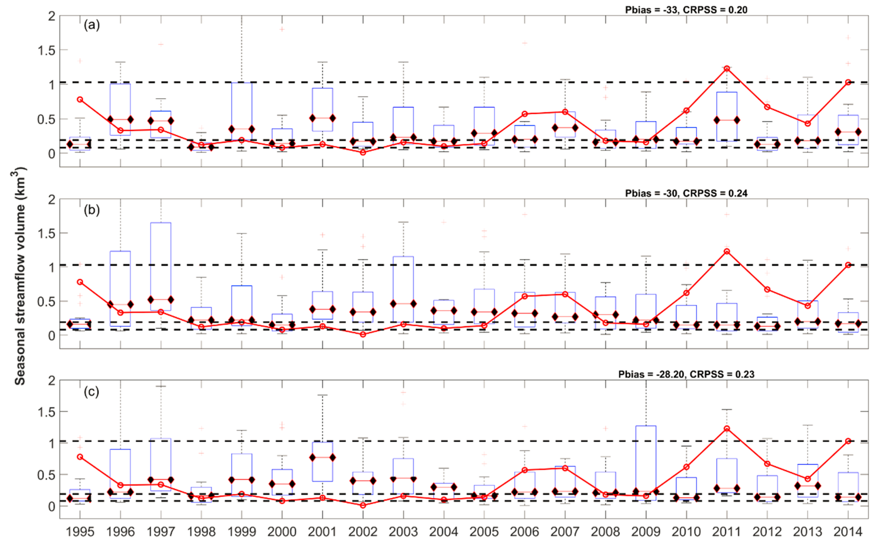
The PBIAS and CRPSS for Scheme-1 using the LR post-processing technique are shown in Figure 8. Results of the post-processed ensembles under Scheme-1 for WATFLOOD and SWAT models are displayed in Figure 8a,b, respectively. Post-processing did not improve WATFLOOD’s skill, while a near 20% increase in the SWAT CRPSS was observed. The LR post-processing technique operates on the ensemble mean and generates adjusted mean and spread statistics [41]. Since SWAT is more capable of predicting low-to-median flow, it is very likely that the model benefits more from post-processing, resulting in higher overall skill. However, it should be noted, given the importance of peak flow prediction in operational forecasting, that post-processing reduced the skill of SWAT in predicting the 2011 peak runoff event (Figure 8b). In general, the post-processed MM ensemble (Figure 8c) showed improved skill (CRPSS of 0.23) in comparison to the predictive skill of individual hydrologic models (CRPSSs of 0.20, and 0.22 for WATFLOOD and SWAT models, respectively). The results also highlight how MM approaches compensate for the individual error among the models. As noted above, the post-processed WATFLOOD ESP over predicted low-flow events (Figure 8a), while the SWAT ESP underpredicted peak runoff events (Figure 8b). When post-processing was applied to the MM ensemble, however, we observed improved skill and lower bias. These results agree with those from other researchers who found that the forecast errors from individual models can “cancel out” [9,62,63]. This is why MM ensemble means are often regarded as more skillful predictions than the results from individual models [64].
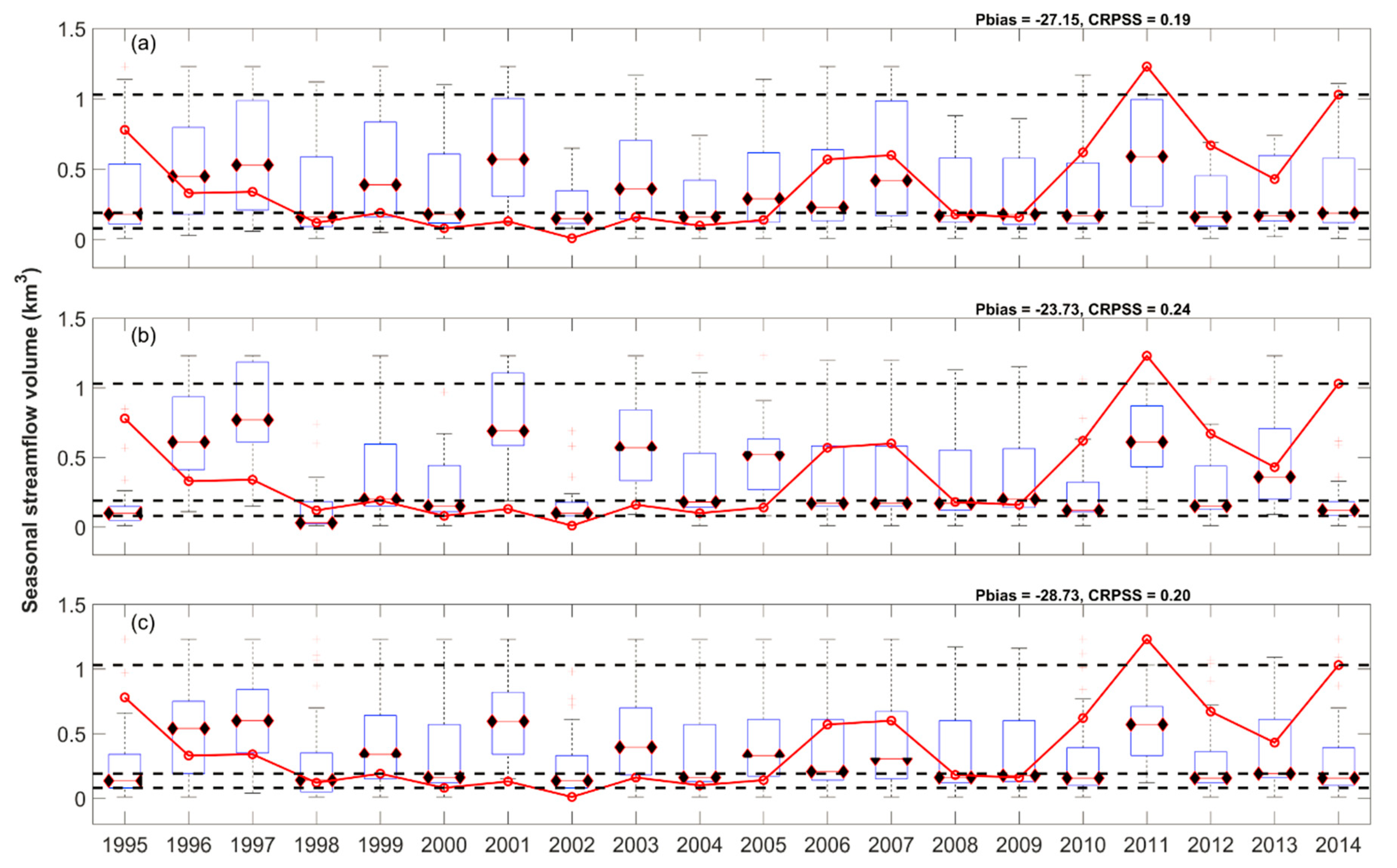
Figure 9 represents the post-processed ESPs for WATFLOOD and SWAT using QM. The QM post-processing technique does not improve the predictability of WATFLOOD runoff volume (Figure 9a); however, a modest improvement was observed for SWAT (Figure 9b), with the CRPSS improving from 0.20 to 0.24. QM similarly does not produce noticeable improvement in the forecast accuracy for the MM ensemble (Figure 9c). The QM approach is simple: the CDF of the forecast is adjusted to make the observed CDF. QM does not preserve the connection between each pair of forecast and observed values; thus, QM may sometimes adjust the raw forecast in the wrong direction, producing less satisfactory results [65,66]. This is why more advanced post-processing techniques may be preferable.

3.4. Evaluation of Weighted MM ESPs

In Scheme-1, we presented results when post-processing techniques (LR and QM only) were applied on individual model ESPs, as well as an MM ESP when ensembles are combined in a linear fashion (i.e., without assigning weight to models based on their performance). Merging MM ensembles without considering the performance of individual models, however, is considered to be of less value [67]; hence, there are a number of schemes developed to appreciate individual model performance [20,22,44].
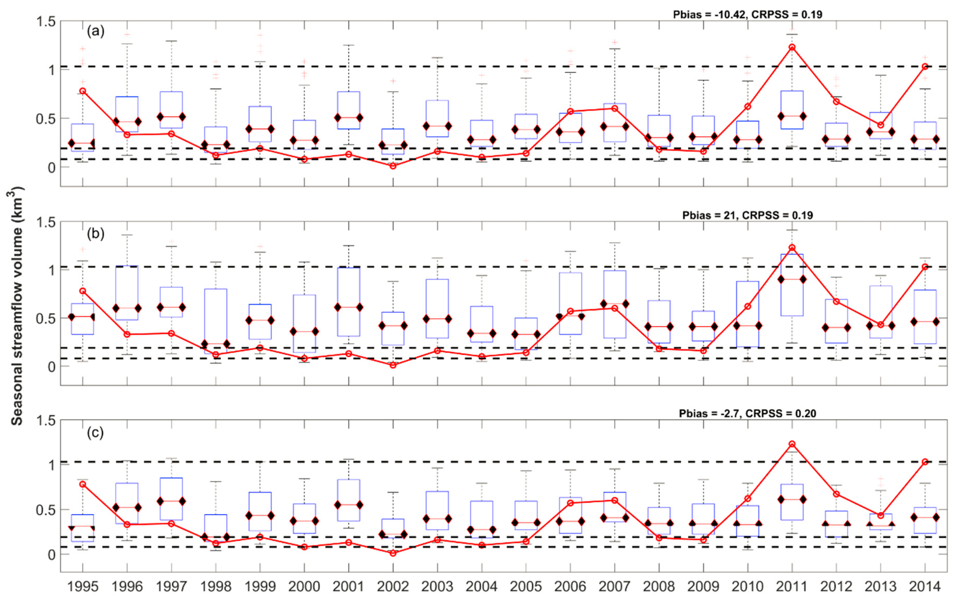
Scheme-2 represents the application of the BMA and QMA post-processing techniques to the merged ensemble formed from the two hydrological models, or the MM ESP. Initial weights for the two models were computed using RMSE to appreciate individual model performance. Based on the simulation performance, SWAT receives a RMSE of 0.53 while WATFLOOD has a RMSE of 0.47. The benchmark MM ESP (Figure 10a) appears to have captured most observed events; however, there are instances, particularly peak-flow events (i.e., 1995, 2011, and 2014) where the benchmark ensemble did not perform as well. The post-processed MM ESP using BMA (Figure 10b) appears to improve the predictability of these peak events that were missed by the benchmark ensemble; however, the overall PBIAS and CRPSS did not improve. Various studies suggest that the performance of BMA can be further improved if climatology is used as one of the candidate models [23,44,68,69]. In fact, the use of climatology would help in reducing the overconfidence of individual model forecasts [70]. QMA post-processing (Figure 10c) showed a slightly improved overall hindcast, with better skill (0.20) and lower bias (−2.7). The QMA hindcast is a weighted average of quantiles from all models [43] which not only corrects the CDF of the forecast with respect to observations but places weights on the hydrological model output based on their performance. In their recent experiment [43], nearly identical skill can be obtained using BMA and QMA, which is a confirmation of results in our experiment using the two techniques. The slight improvement (lower bias) in QMA could be due to the CDF correction, which is an added step as compared to BMA.

3.5. Post-Processing Effectiveness for Operational Prediction

In general, we find the post-processing techniques in many cases have improved the streamflow hindcasts; however, the improvement is not as significant as expected. There could be many reasons for this result. Probabilistic forecasts were verified against observations in this study (to evaluate CRPSS and PBIAS). As models are only abstracts of the reality, and given the complex and highly non-linear response of UARB hydrology, there will be bias introduced into hindcasting due to the models’ not fully replicating reality. Comparing the model ESP to post-processed ESPs statistically would result in improved skill scores for the post-processing techniques. For example, in Figure 5 and Figure 6, the benchmark ESPs are centrally located between post-processed ESPs, and thus the skill of post-processed ESPs would be much stronger relative to the benchmarks (as compared to the observations). Results are similar to those obtained by [71] where the application of various post-processing techniques did not necessarily improve predictability.
Another possible explanation could be that our study focused on hindcast verification at a single, seasonal time step using the three-month lead time. It is possible that the forecast skill and the application of various statistical post-processing techniques would be more notable at multiple, and shorter lead times. For example, a number of post-processing techniques for seasonal flow volume for a singular hydrologic model were evaluated by [20]. In their work, improvement in forecast accuracy at three-month lead time is low to nil. Though many studies have reported the benefit of using MM ESP approaches, it is often far from a trivial challenge to select a suite of models and a method for combining their output. The impact of design choice on the performance of MM forecast configurations, which included decisions about forecast quality attributes, weighting methods, and the number of models, had a significant impact on the identification of an optimal approach [72]. Other studies also highlight the importance of design choices, including the number of hydrological models to be used [73,74,75,76]. Most of the above studies recommended using at least five hydrologic models. Moreover, post-processing of any type of hydrological forecast is based on the assumption of stationarity in climate, weather patterns, and hydrologic response [20,22,44]. This means that the statistical correlation between observations and forecasts during the training and verification periods should remain constant, which is not always valid in hydrology [77], and arguably may not have been the case over this study period for the UARB with two >130-year return period floods (i.e., 2011, and 2014) [78,79]. Such assumptions can introduce errors into the post-processed forecast, leading to greater uncertainty than is expected [44].
As the CRPSS scores of all the post-processing techniques are quite similar, the two-sample Kolmogorov–Smirnov (KS) test was used to test the significance of the change to the simulated distributions after post-processing was conducted.
The KS test results return a decision for the null hypothesis that the data of the two samples are from the same continuous distribution. The alternative hypothesis is that the two samples are from different continuous distributions. H is 1 if the test rejects the null hypothesis at the 5% significance level, and 0 otherwise. The p-value indicates the significance of the test result (Table 1). Here, the null hypothesis was rejected in the case of WATFLOOD under Scheme-1, indicating there is no significant change in the distribution of simulated flows after post-processing. Both the SWAT and MM ESP, however, indicate weak but statistically significant changes in simulated distributions (p-value was close to the critical rejection threshold) with the application of QM. This result is perhaps not surprising given QM explicitly targets distribution quantiles and adjusts them to be closer to the desired distribution of values. Given WATFLOOD reasonably replicated peak volumes before post-processing, it is likely that, given the small sample of the ESP, post-processing had a lower impact. The MM ESP under Scheme-1 showed weak but significant changes in the distribution of flow volume. For Scheme-2, the BMA shows a significant impact on the simulated distribution of simulated flows produced from the MM ensemble; however QMA failed to alter the distribution of peak runoff with any significance.

4. Conclusions

ESP is a key component of operational, long-lead streamflow prediction, which is currently utilized by HFCs in the US, UK, Australia, and other countries. In Canada, its application to date has been limited. In this study, we evaluated the value of ESP in operational forecasting and compared four statistical post-processing techniques for their abilities to improve seasonal flow (volume) prediction. We found that using an ensemble over a deterministic forecast would likely enhance operational decision-making capacity as it reduced uncertainty while providing an envelope of realistic, possible future scenarios. Furthermore, the use of the MM ESP helped to compensate for errors interjected into the forecast by selection of any hydrological model, likely due to structural differences impacting predictive capacity for high and low flow volume differently, and error trade-off.
In most cases, statistical post-processing slightly improved forecast accuracy; however, there were instances where the benchmark ensembles better represented the observed streamflow. Both simpler (i.e., LR and QM) and more complex (BMA and QMA) methods were tested to evaluate the incremental benefits of more complex (parameter-intensive) techniques. While the QMA approach appears to be promising, this study cannot yet confidently recommend any particular post-processing technique due to limitations imposed by the number of models used, the ensemble sample size, basin complexity, and the time period used for analysis. Based on this analysis, we can recommend that testing the performance of the statistical post-processing techniques in the future should be conducted across multiple (smaller) basins, and lead times, using more hydrological models, and larger sample sizes. Care should be taken to select a relatively stationary hydrologic period, without multiple extreme events so as not to violate the stationarity assumption required for model training.

Author Contributions

T.S. provided valuable insights on overall improvement to the representation of this manuscript. F.U. provided access to the HFC operational models. P.C. help in connecting with HFC and editing the manuscript. All the co-authors review the manuscript prior to and during the submission process to the Water-MDPI Journal.

Funding

This research was funded by the Natural Sciences and Engineering Research Council of Canada under Canadian FloodNet project (Grant number: NETGP 451456).

Acknowledgments

The Manitoba HFC, Agriculture, and Agri-Food Canada for providing research-related data is greatly acknowledged. The authors extend gratitude to Pablo Mandoza for providing R-scripts for post-processing techniques and expert guidance on its use. The authors would like to dedicate the paper to the memory of Peter Rasmussen who was key in the journey of the principal author’s PhD.

Conflicts of Interest

The authors declare no conflicts of interest

References

  1. Pagano, T.C.; Pappenberger, F.; Wood, A.W.; Ramos, M.-H.; Persson, A.; Anderson, B. Automation and human expertise in operational river forecasting. Wiley Interdiscip. Rev. Water 2016, 3, 692–705. [Google Scholar] [CrossRef] [Green Version]
  2. Bourdin, D.R.; Fleming, S.W.; Stull, R.B. Streamflow modelling: A primer on applications, approaches and challenges. Atmos. Ocean 2012, 50, 507–536. [Google Scholar] [CrossRef]
  3. Clark, M.P.; Nijssen, B.; Lundquist, J.D.; Kavetski, D.; Rupp, D.E.; Woods, R.A.; Freer, J.E.; Gutmann, E.D.; Wood, A.W.; Gochis, D.J.; et al. A unified approach for process-based hydrologic modeling: 2. Model implementation and case studies. Water Resour. Res. 2015, 51, 2515–2542. [Google Scholar] [CrossRef] [Green Version]
  4. Beven, K. Changing ideas in hydrology—The case of physically-based models. J. Hydrol. 1989, 105, 157–172. [Google Scholar] [CrossRef]
  5. Beven, K.; Binley, A. The future of distributed models: Model calibration and uncertainty prediction. Hydrol. Process. 1992, 6, 279–298. [Google Scholar] [CrossRef]
  6. Butts, M.B.; Payne, J.T.; Kristensen, M.; Madsen, H. An evaluation of the impact of model structure on hydrological modelling uncertainty for streamflow simulation. J. Hydrol. 2004, 298, 242–266. [Google Scholar] [CrossRef]
  7. Crochemore, L.; Ramos, M.-H.; Pappenberger, F. Bias correcting precipitation forecasts to improve the skill of seasonal streamflow forecasts. Hydrol. Earth Syst. Sci. 2016, 20, 3601–3618. [Google Scholar] [CrossRef] [Green Version]
  8. Petrie, R. Localization in the Ensemble Kalman Filter. Master’s Thesis, Univ. of Reading, Reading, UK, 2008. [Google Scholar]
  9. Georgakakos, K.P.; Seo, D.-J.J.; Gupta, H.; Schaake, J.; Butts, M.B. Towards the characterization of streamflow simulation uncertainty through multimodel ensembles. J. Hydrol. 2004, 298, 222–241. [Google Scholar] [CrossRef]
  10. Liu, Y.; Gupta, H.V. Uncertainty in hydrologic modeling: Toward an integrated data assimilation framework. Water Resour. Res. 2007, 43. [Google Scholar] [CrossRef] [Green Version]
  11. Dietrich, J.; Schumann, A.H.; Redetzky, M.; Walther, J.; Denhard, M.; Wang, Y.; Utzner, B.P.; Uttner, U. Assessing uncertainties in flood forecasts for decision making: Prototype of an operational flood management system integrating ensemble predictions. Nat. Hazards Earth Syst. Sci. 2009, 9, 1529–1540. [Google Scholar] [CrossRef]
  12. Kauffeldt, A.; Wetterhall, F.; Pappenberger, F.; Salamon, P.; Thielen, J. Technical review of large-scale hydrological models for implementation in operational flood forecasting schemes on continental level. Environ. Model. Softw. 2016, 75, 68–76. [Google Scholar] [CrossRef]
  13. Kasiviswanathan, K.S.; Sudheer, K.P. Methods used for quantifying the prediction uncertainty of artificial neural network based hydrologic models. Stoch. Environ. Res. Risk Assess. 2017, 31, 1659–1670. [Google Scholar] [CrossRef]
  14. Liu, Y.R.; Li, Y.P.; Huang, G.H.; Zhang, J.L.; Fan, Y.R. A Bayesian-based multilevel factorial analysis method for analyzing parameter uncertainty of hydrological model. J. Hydrol. 2017, 553, 750–762. [Google Scholar] [CrossRef]
  15. Day, G.N. Extended Streamflow Forecasting Using NWSRFS. J. Water Resour. Plan. Manag. 1985, 111, 157–170. [Google Scholar] [CrossRef]
  16. Cloke, H.L.; Pappenberger, F.; van Andel, S.J.; Schaake, J.; Thielen, J.; Ramos, M.H. Hydrological ensemble prediction systems. Hydrol. Process. 2013, 27, 1–4. [Google Scholar] [CrossRef]
  17. Cloke, H.L.; Pappenberger, F. Ensemble flood forecasting: A review. J. Hydrol. 2009, 375, 613–626. [Google Scholar] [CrossRef]
  18. WMO. Guidelines on Ensemble Prediction Systems and Forecasting; World Meteorological Organization (WMO): Geneva, Switzerland, 2012. [Google Scholar]
  19. Harrigan, S.; Prudhomme, C.; Parry, S.; Smith, K.; Tanguy, M. Benchmarking Ensemble Streamflow Prediction skill in the UK. Hydrol. Earth Syst. Sci. Discuss. 2017. [Google Scholar] [CrossRef]
  20. Mendoza, P.A.; Wood, A.W.; Clark, E.; Rothwell, E.; Clark, M.P.; Nijssen, B.; Brekke, L.D.; Arnold, J.R. An intercomparison of approaches for improving operational seasonal streamflow forecasts. Hydrol. Earth Syst. Sci. 2017, 21, 3915–3935. [Google Scholar] [CrossRef] [Green Version]
  21. Lucatero, D.; Madsen, H.; Refsgaard, J.C.; Kidmose, J.; Jensen, K.H. Seasonal streamflow forecasts in the Ahlergaarde catchment, Denmark: The effect of preprocessing and postprocessing on skill and statistical consistency. Hydrol. Earth Syst. Sci. 2018. [Google Scholar] [CrossRef]
  22. Li, W.; Duan, Q.; Miao, C.; Ye, A.; Gong, W.; Di, Z. A review on statistical postprocessing methods for hydrometeorological ensemble forecasting. Wiley Interdiscip. Rev. Water 2017, 4, e1246. [Google Scholar] [CrossRef]
  23. Mendoza, P.A.; Rajagopalan, B.; Clark, M.P.; Ikeda, K.; Rasmussen, R.M.; Mendoza, P.A.; Rajagopalan, B.; Clark, M.P.; Ikeda, K.; Rasmussen, R.M. Statistical Postprocessing of High-Resolution Regional Climate Model Output. Mon. Weather Rev. 2015, 143, 1533–1553. [Google Scholar] [CrossRef]
  24. Jha, S.K.; Shrestha, D.L.; Stadnyk, T.; Coulibaly, P. Evaluation of ensemble precipitation forecasts generated through postprocessing in a Canadian catchment. Hydrol. Earth Syst. Sci. Discuss. 2017. [Google Scholar] [CrossRef]
  25. Coulibaly, P. NSERC FloodNet Manual; Natural Sciences and Engineering Research Council of Canada: Hamilton, ON, Canada, 2014. [Google Scholar]
  26. Saskatchewan Water Security Agency. Upper Assiniboine River Basin Study; Sask Water: Moose Jaw, SK, Canada, 2000. Available online: https://www.gov.mb.ca/waterstewardship/reports/planning_development/uarb_report.pdf (accessed on 8 November 2018).
  27. Shrestha, R.R.; Dibike, Y.B.; Prowse, T.D. Modeling Climate Change Impacts on Hydrology and Nutrient Loading in the Upper Assiniboine Catchmen. J. Am. Water Resour. Assoc. 2012, 48, 74–89. [Google Scholar] [CrossRef]
  28. Stadnyk-Falcone, T.A. Mesoscale Hydrological Model Validation and Verification Using Stable Water Isotopes: The isoWATFLOOD Model. Ph.D. Thesis, University of Waterloo, Waterloo, ON, Canada, 2008. [Google Scholar]
  29. Kouwen, N. WATFLOOD Users Manual; Water Resources Group, Department of Civil Engineering, University of Waterloo: Waterloo, ON, Canada, 1998. [Google Scholar]
  30. Kouwen, N. Flow Forecasting Manual for WATFLOOD and GreenKenue. Available online: http://www.civil.uwaterloo.ca/watflood/downloads/Flow_Forecasting_Manual.pdf (accessed on 8 November 2018).
  31. Gassman, P.W.; Arnold, J.G.; Srinivasan, R.; Reyes, M. The worldwide use of the SWAT Model: Technological drivers, networking impacts, and simulation trends. In Proceedings of the Watershed Technology Conference, Guácimo, Costa Rica, 21–24 February 2010; pp. 21–24. [Google Scholar]
  32. Neitsch, S.L.; Arnold, J.G.; Kiniry, J.R.; Williams, J.R. Soil and Water Assessment Tool Theoretical Documentation Version 2009; Texas Water Resources Institute: College Station, TX, USA, 2011; Available online: http://hdl.handle.net/1969.1/128050 (accessed on 8 November 2018).
  33. White, E.D.; Easton, Z.M.; Fuka, D.R.; Collick, A.S.; Adgo, E.; McCartney, M.; Awulachew, S.B.; Selassie, Y.G.; Steenhuis, T.S. Development and application of a physically based landscape water balance in the SWAT model. Hydrol. Process. 2011, 25, 915–925. [Google Scholar] [CrossRef]
  34. Williams, J.R. Flood routing with variable travel time or variable storage coefficients. Trans. ASAE 1969, 12, 100–103. [Google Scholar] [CrossRef]
  35. Evenson, G.R.; Golden, H.E.; Lane, C.R.; D’Amico, E. An improved representation of geographically isolated wetlands in a watershed-scale hydrologic model. Hydrol. Process. 2016, 30, 4168–4184. [Google Scholar] [CrossRef]
  36. Evenson, G.R.; Golden, H.E.; Lane, C.R.; Amico, E.D.; D’Amico, E. Geographically isolated wetlands and watershed hydrology: A modified model analysis. J. Hydrol. 2015, 529, 240–256. [Google Scholar] [CrossRef] [Green Version]
  37. Qu, B.; Zhang, X.; Pappenberger, F.; Zhang, T.; Fang, Y. Multi-Model Grand Ensemble Hydrologic Forecasting in the Fu River Basin Using Bayesian Model Averaging. Water 2017, 9, 74. [Google Scholar] [CrossRef]
  38. Hsu, K.; Moradkhani, H.; Sorooshian, S. A sequential Bayesian approach for hydrologic model selection and prediction. Water Resour. Res. 2009, 45. [Google Scholar] [CrossRef] [Green Version]
  39. Zhang, X.; Srinivasan, R.; Bosch, D. Calibration and uncertainty analysis of the SWAT model using Genetic Algorithms and Bayesian Model Averaging. J. Hydrol. 2009, 374, 307–317. [Google Scholar] [CrossRef]
  40. Tian, X.; Xie, Z.; Wang, A.; Yang, X. A new approach for Bayesian model averaging. Sci. China Earth Sci. 2012, 55, 1336–1344. [Google Scholar] [CrossRef]
  41. Wood, A.W.; Schaake, J.C. Correcting Errors in Streamflow Forecast Ensemble Mean and Spread. J. Hydrometeorol. 2008, 9, 132–148. [Google Scholar] [CrossRef]
  42. Raftery, A.E.; Gneiting, T.; Balabdaoui, F.; Polakowski, M. Using Bayesian Model Averaging to Calibrate Forecast Ensembles. Mon. Weather Rev. 2005, 133, 1155–1174. [Google Scholar] [CrossRef] [Green Version]
  43. Schepen, A.; Wang, Q.J. Model averaging methods to merge operational statistical and dynamic seasonal streamflow forecasts in Australia. Water Resour. Res. 2015, 51, 1797–1812. [Google Scholar] [CrossRef] [Green Version]
  44. Wood, A.W.; Sankarasubramanian, A.; Mendoza, P. Seasonal Ensemble Forecast Post-processing. In Handbook of Hydrometeorological Ensemble Forecasting; Springer: Berlin/Heidelberg, Germany, 2018; pp. 1–27. [Google Scholar]
  45. Hashino, T.; Bradley, A.A.; Schwartz, S.S. Evaluation of bias-correction methods for ensemble streamflow volume forecasts. Hydrol. Earth Syst. Sci. 2007, 11, 939–950. [Google Scholar] [CrossRef] [Green Version]
  46. Najafi, M.R.; Moradkhani, H. Ensemble Combination of Seasonal Streamflow Forecasts. J. Hydrol. Eng. 2016, 21, 04015043. [Google Scholar] [CrossRef]
  47. Jiang, S.; Ren, L.; Xu, C.-Y.; Liu, S.; Yuan, F.; Yang, X. Quantifying multi-source uncertainties in multi-model predictions using the Bayesian model averaging scheme. Hydrol. Res. 2017, nh2017272. [Google Scholar] [CrossRef]
  48. Moriasi, D.N.; Arnold, J.G.; Van Liew, M.W.; Binger, R.L.; Harmel, R.D.; Veith, T.L. Model evaluation guidelines for systematic quantification of accuracy in watershed simulations. Trans. ASABE 2007, 50, 885–900. [Google Scholar] [CrossRef]
  49. Veerasamy, R.; Rajak, H.; Jain, A.; Sivadasan, S.; Varghese, C.P.; Agrawal, R.K. Validation of QSAR Models—Strategies and Importance. Int. J. Drug Des. Disocov. 2011, 2, 511–519. [Google Scholar] [CrossRef] [Green Version]
  50. Hersbach, H. Decomposition of the Continuous Ranked Probability Score for Ensemble Prediction Systems. Weather Forecast. 2000, 15, 559–570. [Google Scholar] [CrossRef]
  51. Alfieri, L.; Pappenberger, F.; Wetterhall, F.; Haiden, T.; Richardson, D.; Salamon, P. Evaluation of ensemble streamflow predictions in Europe. J. Hydrol. 2014, 517, 913–922. [Google Scholar] [CrossRef]
  52. Kouwen, N. WATFLOOD: A Micro-Computer Based Flood Forecasting System Based on Real-Time Weather Radar. Can. Water Resour. J. 1988, 13, 62–77. [Google Scholar] [CrossRef]
  53. Shook, K.; Pomeroy, J.W.; Spence, C.; Boychuk, L. Storage dynamics simulations in prairie wetland hydrology models: Evaluation and parameterization. Hydrol. Process. 2013, 27, 1875–1889. [Google Scholar] [CrossRef]
  54. Unduche, F.; Tolossa, H.; Senbeta, D.; Zhu, E. Evaluation of four hydrological models for operational flood forecasting in a Canadian Prairie watershed. Hydrol. Sci. J. 2018, 1–17. [Google Scholar] [CrossRef]
  55. Wood, A.W.; Hopson, T.; Newman, A.; Brekke, L.; Arnold, J.; Clark, M. Quantifying Streamflow Forecast Skill Elasticity to Initial Condition and Climate Prediction Skill. J. Hydrometeorol. 2016, 17, 651–668. [Google Scholar] [CrossRef]
  56. Greuell, W.; Franssen, W.H.P.; Hutjes, R.W.A. Seasonal streamflow forecasts for Europe—II. Explanation of the skill. Hydrol. Earth Syst. Sci. Discuss. 2016. [Google Scholar] [CrossRef]
  57. Wood, A.W.; Lettenmaier, D.P. An ensemble approach for attribution of hydrologic prediction uncertainty. Geophys. Res. Lett. 2008, 35, L14401. [Google Scholar] [CrossRef]
  58. Najafi, M.R.; Moradkhani, H. Multi-model ensemble analysis of runoff extremes for climate change impact assessments. J. Hydrol. 2015, 525, 352–361. [Google Scholar] [CrossRef] [Green Version]
  59. Borah, D.K.; Bera, M.; Xia, R. Storm event flow and sediment simulations in agricultural watersheds using DWSM. Trans. ASAE 2004, 47, 1539–1559. [Google Scholar] [CrossRef]
  60. Yaduvanshi, A.; Sharma, R.K.; Kar, S.C.; Sinha, A.K. Rainfall–runoff simulations of extreme monsoon rainfall events in a tropical river basin of India. Nat. Hazards 2018, 90, 843–861. [Google Scholar] [CrossRef]
  61. Shook, K.; Pomeroy, J.W. Memory effects of depressional storage in Northern Prairie hydrology. Hydrol. Process. 2011, 25, 3890–3898. [Google Scholar] [CrossRef]
  62. Shamseldin, A.Y.; O’Connor, K.M.; Liang, G.C. Methods for combining the outputs of different rainfall–runoff models. J. Hydrol. 1997, 197, 203–229. [Google Scholar] [CrossRef]
  63. Duan, Q.; Ajami, N.K.; Gao, X.; Sorooshian, S. Multi-model ensemble hydrologic prediction using Bayesian model averaging. Adv. Water Resour. 2007, 30, 1371–1386. [Google Scholar] [CrossRef]
  64. Bohn, T.J.; Sonessa, M.Y.; Lettenmaier, D.P. Seasonal Hydrologic Forecasting: Do Multimodel Ensemble Averages Always Yield Improvements in Forecast Skill? J. Hydrometeorol. 2010, 11, 1358–1372. [Google Scholar] [CrossRef]
  65. Madadgar, S.; Moradkhani, H. Improved Bayesian multimodeling: Integration of copulas and Bayesian model averaging. Water Resour. Res. 2014, 50, 9586–9603. [Google Scholar] [CrossRef] [Green Version]
  66. Zhao, T.; Bennett, J.C.; Wang, Q.J.; Schepen, A.; Wood, A.W.; Robertson, D.E.; Ramos, M.-H.; Zhao, T.; Bennett, J.C.; Wang, Q.J.; et al. How Suitable is Quantile Mapping for Postprocessing GCM Precipitation Forecasts? J. Clim. 2017, 30, 3185–3196. [Google Scholar] [CrossRef]
  67. Krysanova, V.; Donnelly, C.; Gelfan, A.; Gerten, D.; Arheimer, B.; Hattermann, F.; Kundzewicz, Z.W. How the performance of hydrological models relates to credibility of projections under climate change. Hydrol. Sci. J. 2018, 63, 696–720. [Google Scholar] [CrossRef]
  68. Rajagopalan, B.; Lall, U. Categorical Climate Forecasts through Regularization and Optimal Combination of Multiple GCM Ensembles. Mon. Weather Rev. 2002, 130, 1792–1811. [Google Scholar] [CrossRef]
  69. Grantz, K.; Rajagopalan, B.; Clark, M.; Zagona, E. A technique for incorporating large-scale climate information in basin-scale ensemble streamflow forecasts. Water Resour. Res. 2005, 41. [Google Scholar] [CrossRef]
  70. Weigel, A.P.; Liniger, M.A.; Appenzeller, C. Can multi-model combination really enhance the prediction skill of probabilistic ensemble forecasts? Q. J. R. Meteorol. Soc. 2008, 134, 241–260. [Google Scholar] [CrossRef] [Green Version]
  71. Verkade, J.S.; Brown, J.D.; Reggiani, P.; Weerts, A.H. Post-processing ECMWF precipitation and temperature ensemble reforecasts for operational hydrologic forecasting at various spatial scales. J. Hydrol. 2013, 501, 73–91. [Google Scholar] [CrossRef]
  72. Mendoza, P.A.; Rajagopalan, B.; Clark, M.P.; Cortés, G.; McPhee, J. A robust multimodel framework for ensemble seasonal hydroclimatic forecasts. Water Resour. Res. 2014, 50, 6030–6052. [Google Scholar] [CrossRef] [Green Version]
  73. Velázquez, J.A.; Anctil, F.; Perrin, C. Performance and reliability of multimodel hydrological ensemble simulations based on seventeen lumped models and a thousand catchments. Hydrol. Earth Syst. Sci. 2010, 14, 2303–2317. [Google Scholar] [CrossRef] [Green Version]
  74. Hagedorn, R.; Doblas-Reyes, F.J.; Palmer, T.N. The rationale behind the success of multi-model ensembles in seasonal forecasting—I. Basic concept. Tellus Ser. A Dyn. Meteorol. Oceanogr. 2005, 57, 219–233. [Google Scholar] [CrossRef]
  75. Bormann, H.; Breuer, L.; Croke, B. Reduction of predictive uncertainty by ensemble hydrological Uncertainties in the modelling’ sequence of catchment research. In Proceedings of the 11th Conference of the Euromediterranean Network of Experimental and Representative Basins (ERB), Luxembourg, Luxembourg, 20–22 September 2006. [Google Scholar]
  76. Krishnamurti, T.N.; Kishtawal, C.M.; LaRow, T.E.; Bachiochi, D.R.; Zhang, Z.; Williford, C.E.; Gadgil, S.; Surendran, S. Improved Weather and Seasonal Climate Forecasts from Multimodel Superensemble. Science 1999, 285, 1548–1550. [Google Scholar] [CrossRef] [PubMed]
  77. Milly, A.P.C.D.; Betancourt, J.; Falkenmark, M.; Hirsch, R.M.; Zbigniew, W.; Lettenmaier, D.P.; Stouffer, R.J.; Milly, P.C.D. Stationarity Is Dead: Stationarity Whither Water Management? Science 2008, 319, 573–574. [Google Scholar] [CrossRef] [PubMed]
  78. Blais, E.-L.; Clark, S.; Dow, K.; Rannie, B.; Stadnyk, T.; Wazney, L. Background to flood control measures in the Red and Assiniboine River Basins. Can. Water Resour. J. 2016, 41, 31–44. [Google Scholar] [CrossRef]
  79. Blais, E.-L.; Greshuk, J.; Stadnyk, T. The 2011 flood event in the Assiniboine River Basin: Causes, assessment and damages. Can. Water Resour. J. 2016, 41, 74–84. [Google Scholar] [CrossRef]
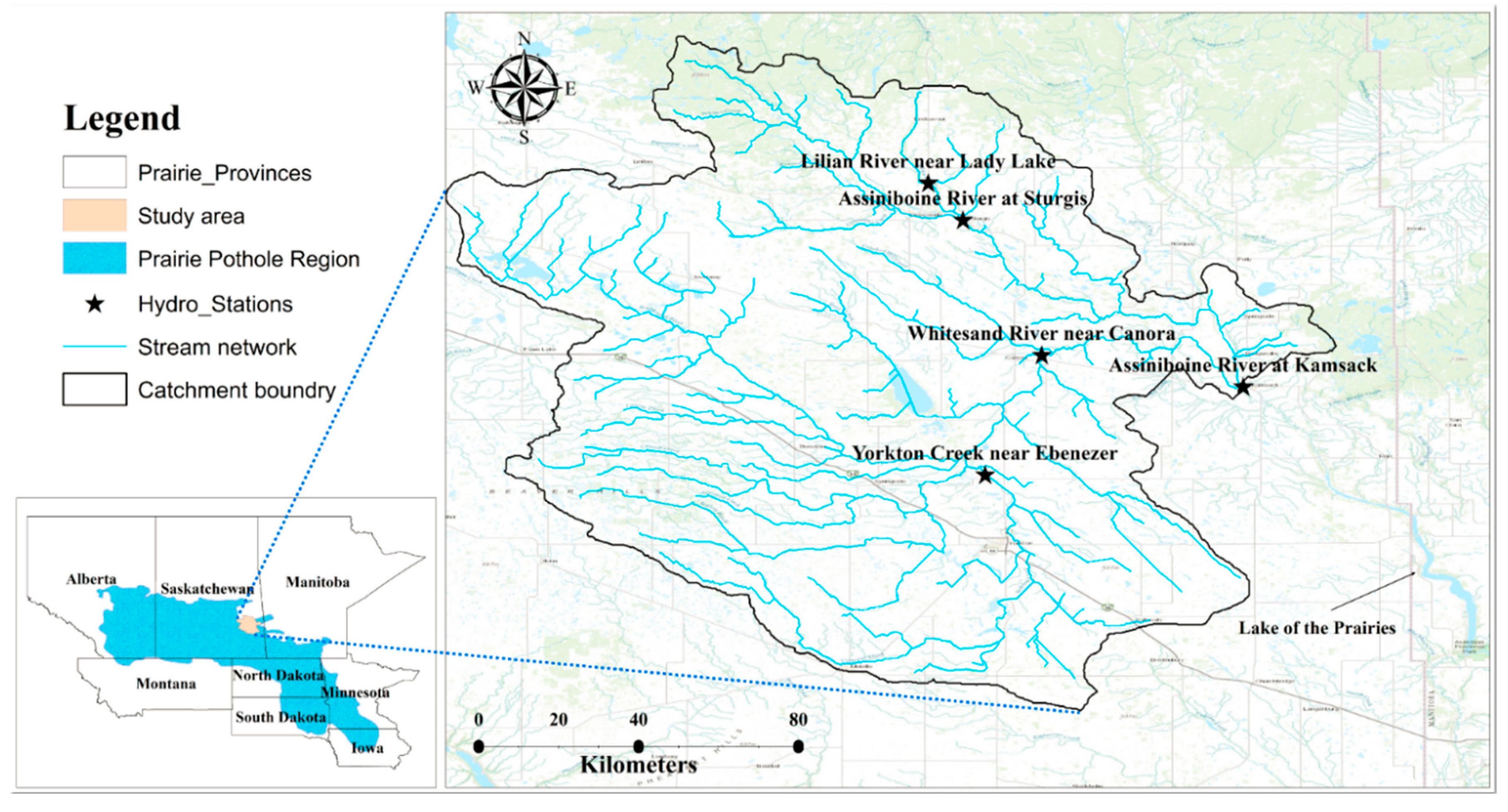
Figure 1. Geographical location of the Upper Assiniboine River Basin (UARB) with respect to the Prairie Pothole Region (PPR).
Water 10 01604 g001
Figure 2. Stream flow versus precipitation at the UARB at Kamsack (WSC ID: 05MD004) over 1981–2010.
Water 10 01604 g002
Figure 3. Schematic of ensemble forecast generation and the application of post-processing technique.
Water 10 01604 g003
Figure 4. Daily average annual streamflow hydrograph from 1994 to 2004 at the catchment outlet (WSC ID: 05MD004) using two hydrologic models. The NSE and R2 are computed using daily observed simulated data over the entire period. The markings on the x-axis indicate the midpoint of each month.
Water 10 01604 g004
Figure 5. Taylor diagram of observed streamflow volume relative to the mean of benchmark (raw) ESP performance (1994–2004) for two hydrologic models and various post-processing techniques. WF stands for WatFlood, and SW stands for SWAT; subscripts LR and QM stand for Linear Regression and Quantile Mapping post-processing techniques, respectively.
Water 10 01604 g005
Figure 6. Taylor diagram of observed streamflow volume relative to the mean of multi-model benchmark ESP performance (1994–2004) for two hydrologic models (combined in linear fashion) and all post-processing techniques. MM indicates the benchmark ESP formed using both WATFLOOD and SWAT models; subscript LR stands for Linear Regression, QM stands for Quantile Mapping, BMA stands for Bayesian Model Averaging, and QMA stands for Quantile Model Averaging.
Water 10 01604 g006
Figure 7. Time series of seasonal streamflow volume for the benchmark ESPs from (a) WATFLOOD, (b) SWAT. Black dashed lines represent 10, 50, and 90% flows from the observed climatology, and the boxplot shows the spread in ensembles. The red line represents the observed volume of discharge.
Water 10 01604 g007
Figure 8. Time series of seasonal streamflow volume for the post-processed ESPs using LR for (a) WATFLOOD, (b) SWAT, and the (c) multi-model ESP using LR. Black dashed lines represent 10, 50, and 90% flows from the observed climatology, and the boxplot shows the spread in ensembles. The red line represents the observed volume of discharge.
Water 10 01604 g008
Figure 9. Time series of seasonal streamflow volume for the post-processed ESPs using QM for (a) WATFLOOD, (b) SWAT, and the (c) multi-model ESP using QM. Black dashed lines represent 10, 50, and 90% flows from the observed climatology, and the boxplot shows the spread in ensembles. The red line represents the observed volume of discharge.
Water 10 01604 g009
Figure 10. Time series of seasonal streamflow volume for (a) multi-model benchmark ESP (WATFLOOD and SWAT combined in a linear fashion), and the post-processed multi-model ESP using (b) BMA and (c) QMA. Black dashed lines represent 10, 50, and 90% flows from the observed climatology, and the boxplot shows the spread in ensembles. The red line represents the observed flow volume.
Water 10 01604 g010
Table 1. Two-sample Kolmogorov–Smirnov (KS) test for resulting significance of the post-processing techniques relative to the raw ensembles.
WATFLOOD (CRPSS)Stat. Sig: H(p)SWAT (CRPSS)Stat. Sig: H(p)Multi-Model (CRPSS)Stat. Sig: H(p)
Scheme-1
LR0.201 (0.0232)0.241 (0.0082)0.230 (0.4973)
QM0.191 (0.0026)0.240 (0.4973)0.200 (0.0591)
Scheme-2
BMA 0.191 (0.0232)
QMA 0.200 (0.7710)