Climate Change and Curtailment: Evaluating Water Management Practices in the Context of Changing Runoff Regimes in a Snowmelt-Dominated Basin

Abstract

Hydrologic scientists and water resource managers often focus on different facets of flow regimes in changing climates. The objective of this work is to examine potential hydrological changes in the Upper Boise River Basin, Idaho, USA in the context of biophysical variables and their impacts a key variable governing administration of water resources in the region in an integrated way. This snowmelt-dominated, mountainous watershed supplies water to a semi-arid, agriculturally intensive, but rapidly urbanizing, region. Using the Envision integrated modeling framework, we created a hydrological model to simulate hydrological response to the year 2100 using six alternative future climate trajectories. Annual discharge increased from historical values by 6–24% across all simulations (with an average 13% increase), reflecting an increase in precipitation in the climate projections. Discharge peaked 4–33 days earlier and streamflow center of timing occurred 4–17 days earlier by midcentury. Examining changes in the date junior water rights holders begin to be curtailed regionally (the Day of Allocation), we found that the it occurs at least 14 days earlier by 2100 across all simulations, with one suggesting it could occur over a month earlier. These results suggest that current methods and policies of water rights accounting and management may need to be revised moving into the future.

1. Introduction

Climate change exerts a significant control on global hydrological regimes by influencing the timing, magnitude, phase, and seasonal variability in precipitation [1,2,3,4,5]. Changes in temperature further influence how that precipitation moves through a watershed by affecting snowmelt timing, soil moisture, and evapotranspiration rates [6,7]. While there is general consensus among scientists that the Earth is warming and will continue to do so, there remain significant uncertainties regarding the impacts of global warming on the water cycle and how those changes will be distributed regionally in the future [8,9].

Significant changes in the water cycle can have serious consequences for water users and management across many sectors. It is estimated that more than two billion people currently live in highly water-stressed regions [10], with this number projected to increase in the future [11]. Agriculture is vulnerable to changes in hydrological regimes, especially in regions that rely on surface water resources for irrigation and in rain-fed systems [9]. Flooding could intensify, putting stress on current water management infrastructure as well as lessening the effectiveness of hydropower generation as runoff arrives earlier [12]. Despite the seriousness of the potential impacts of hydrological changes across sectors, the effectiveness of current water management systems, practices, and policies under changing hydrological regimes is not well understood.

Many previous modeling studies have investigated how water resources will respond to climate change in snowmelt-dominated systems [13,14,15,16]. However, results from such studies are not always presented in a way that is usable to water managers and users. Here we provide an example of how hydrological modelers can generate results that may provide additional meaning for management decisions. Managers of these systems tend to focus on the ways in which climate variability and change will challenge existing water management protocols and practices. For example, in the American West, there are often hierarchies of water rights users who may be affected differently by projected changes in water availability [17]. Providing predictions more applicable to water users requires more in-depth and location-specific knowledge of water management and distribution but has the potential to provide more relevant information to a wider group of audiences.

Snowmelt-dominated systems, particularly those in the western U.S., are especially vulnerable to climate change [6,7,18]. Significant reservoirs, in the form of snow, develop at times (i.e., winter) and locations (i.e., high elevations) where that water cannot be used to grow crops and produce hydroelectricity. This snowpack at high elevations provides a natural reservoir that holds water in reserve and, ideally, slowly releases it into the spring and summer, into downstream agricultural areas. A complex system of water rights and management has been developed, and reservoir and canal systems engineered to store springtime runoff, mitigate flooding, and direct it to other locations when there is a demand for irrigation. This current system of water management infrastructure and protocols are set up to account for the historical range of hydrological variability; however, it may not be adequate to adapt to future hydrological regimes [19]. With sufficient changes in the timing and magnitude of water delivery, as is projected with climate change, current management practices may be inadequate to meet the dual needs of flood control and late-season irrigation demand [6]. However, it is uncertain to what extent current management practices may be stressed under future hydrological regimes or when water management agencies can expect existing practices and policies to begin coming into conflict with the reality of altered runoff regimes.

The overarching objective of this study is to better understand and quantify how climate change will impact future water resources and water management in the context of metrics that managers monitor and use to implement policy. We perform our study in the Upper Boise River Basin, Idaho, USA, an ideal location because it is a relatively undisturbed high mountain watershed that is managed to provide water resources to an agriculturally-intensive and rapidly urbanizing region. We explore this connected biophysical and social system by combining a surface water hydrological model with diverse climate projections to project potential changes in future regional hydrological regimes. Furthermore, we translate our model outputs into a metric that is directly applicable to downstream water users and managers. Our specific research objectives are to:

• Identify a range of climate projections and assess how they affect hydrological parameters such as center of timing of streamflow, volume of annual water delivery, and snowpack levels through the end of the century; and
• Identify how these changes in hydrological regimes impact an associated metric that characterizes water storage and is used to enforce water rights accounting policies.

2. Methods

2.1. Study Area

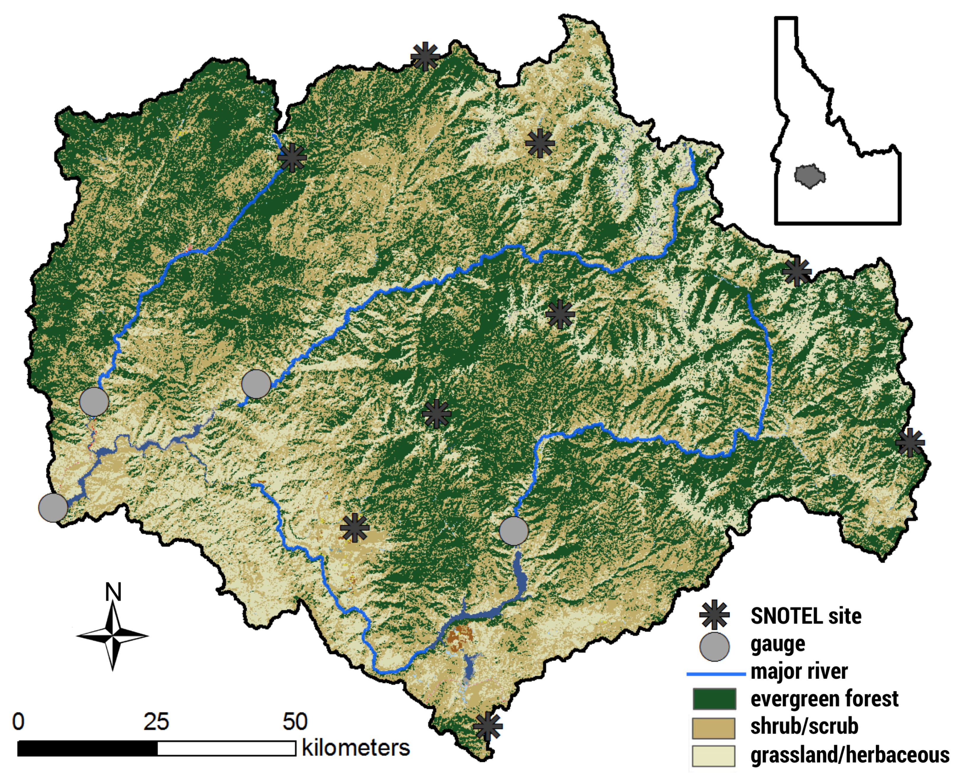
The Upper Boise River Basin (UBRB) is located in southwest Idaho (Figure 1) and supplies water for downstream users in the populated Boise metropolitan region. This watershed encompasses an area of 6935 km${}^2$ with elevation ranging from approximately 930 to 3000 m. It is bounded by the Sawtooth range in the east, the Payette River Basin to the north, and the Snake River Plain to the southwest. We delineated the study area by combining three Hydrologic Unit Code (HUC) 8 watersheds: the North and Middle Forks Boise (U.S. Geological Survey streamflow station 17050111), the South Fork Boise (U.S. Geological Survey streamflow station 17050113), and Boise-Mores (U.S. Geological Survey streamflow station 17050112). Due to the large variation in topography throughout the study area, regions shift from semi-arid grasslands and shrublands in the lowlands to coniferous forests in the highlands. In the UBRB, the dominant land covers are forest (43.0%), shrubland (34.6%) and grassland (20.9%), with sparse human development within the watershed. The climate in this region is a continental Mediterranean climate (Köppen Dsb) with cold winters, warm summers, and the majority of precipitation falling in winter as snow. The overall average precipitation is ∼800 mm, with averages ranging from ∼400 mm at low elevations to over 1300 mm at high elevations [20].

The UBRB is the primary source of water for the downstream Treasure Valley region, which contains the state’s three largest cities (Boise, Nampa, and Meridian) and roughly 40% of the state’s total population. The Treasure Valley is an agriculturally intensive region and contains approximately 1300 km${}^2$ of farmlands, many of which rely on irrigation water from the UBRB. Like many other snowmelt-dominated watersheds in the West, the UBRB is heavily managed via three large storage reservoirs to fulfill the needs of flood control and downstream uses, especially for direct consumption in the Treasure Valley. Similar to other western states, water rights in this region follow the Prior Appropriation Doctrine, also known as “first in time–first in right.” This doctrine states that the earliest beneficial users (i.e., senior water rights) retain their full water right, and those that came later (i.e., junior water rights) may retain their water rights as long as they do not infringe on those that came beforehand. As such, many junior water rights are curtailed during low water years, as total surface water rights in the Treasure Valley surpass 14,000 ft${}^3$/s, far exceeding the natural flow of the Boise River.

Previous studies indicate that the UBRB has already begun to respond hydrologically to climate change, noting an increase in summer streamflow temperatures [21], earlier timing of streamflow [22], lengthened growing season [23], and declining extreme low flow discharges [24]. Additionally, there have been previous modeling studies that have used this basin to anticipate changes in hydrology under climate change [14,25]. However, both of the aforementioned studies used an older generation of global climate models as their climate input and calibrated their models to streamflow alone. This study extends those previous works by making use of climate projections from the 5th Coupled Model Intercomparison Project (CMIP5) [26], calibrating the hydrological model to multiple hydrological metrics, and producing results that may provide additional meaning to water users.

2.2. Modeling Framework

Here we employ the Envision framework, a multiagent-based, spatially explicit modeling framework, to model how regional hydrology may change with climate. Envision was created to explicitly simulate the coupled dynamics of human and natural environmental systems [27]. It does this by providing a core set of utilities to represent landscapes in spatially explicit ways and a software framework for component models of natural systems interact with human actions that occur at places and times specified by a user or a more complex model of human intervention. To this end, the modeling framework and software infrastructure of Envision support the integration of a variety of social and biophysical models in a spatiotemporally dynamic way. It is freely available and users can extend and enhance model capabilities by adding additional models as plugins. It has been extensively used recently in a wide variety of studies, from understanding urbanization impacts on streamflow [28] to projecting climate change impacts of land cover and land use [29], and even to understand when fire occurrence and size is ’surprising’ [30]. Additionally, it has been used to integrate water rights to spatially allocate irrigation in the agriculturally intensive region below the UBRB [31].

In this study, we use Envision version 6.197 and utilize the Flow extension to model future hydrology under various climate scenarios. In the following sections, we provide an overview of the modeling structure and the inputs needed for the various components.

2.2.1. Spatial Coverage in Envision

In Envision, owing to the heritage of the framework for simulating coupled human-natural systems, the most refined spatial elements where model algorithms are applied are referred to as Integrated Decision Units (IDUs). An IDU is meant to represent a contiguous portion of the landscape with relatively constant physiographic (e.g., vegetation cover, soil type, etc.) and socio-political (e.g., land ownership, zoning, land use, etc.) characteristics. The size and geometry of these polygons are dependent on the type of modeling being performed and the geospatial datasets required as input to those models. As such, there is no universally accepted method for creating IDU coverage. In this study, we used three datasets to form the IDU geometry: surface management agency, land cover, and HUC 12 stream catchments (

Table 1. Data sources used for spatial coverage in Envision. IDU, Integrated Decision Unit; ET, Evapotranspiration; HUC, Hydrologic Unit Code; HBV, Hydrologiska Byråns Vattenbalansavdelning; HRU, Hydrologic Response Unit.

Input Data (Resolution)	Data Sources	Used in
Surface Management Agency	Bureau of Land Management	IDU
Land Cover (30 m)	National Landcover Database (2011)	IDU, ET
Streams & Catchments (HUC12)	NHD Plus V2	IDU, HBV
Elevation (30 m)	National Elevation Dataset	HRU

). As such, the IDU coverage will preserve boundaries between HUC 12 catchments, cognizant land management agencies, as well as boundaries between vegetation classes.

The datasets were processed in ArcMap 10.1. To shorten Envision’s computational time, we coarsened the land cover dataset from 30 to 100 m in increments of 10 m. This allowed a substantial reduction in computational time required to create the IDU domain without a significant loss is gradients of vegetation cover, particularly those associated with contrasting vegetation cover on South- and North-facing hillslopes. We used a nearest neighbor algorithm to resample land cover types to more accurately capture the original distribution of coverage in the land cover dataset. The other two datasets were polygon geospatial datasets that required very little processing besides renaming attributes to be consistent with the Envision framework requirements.

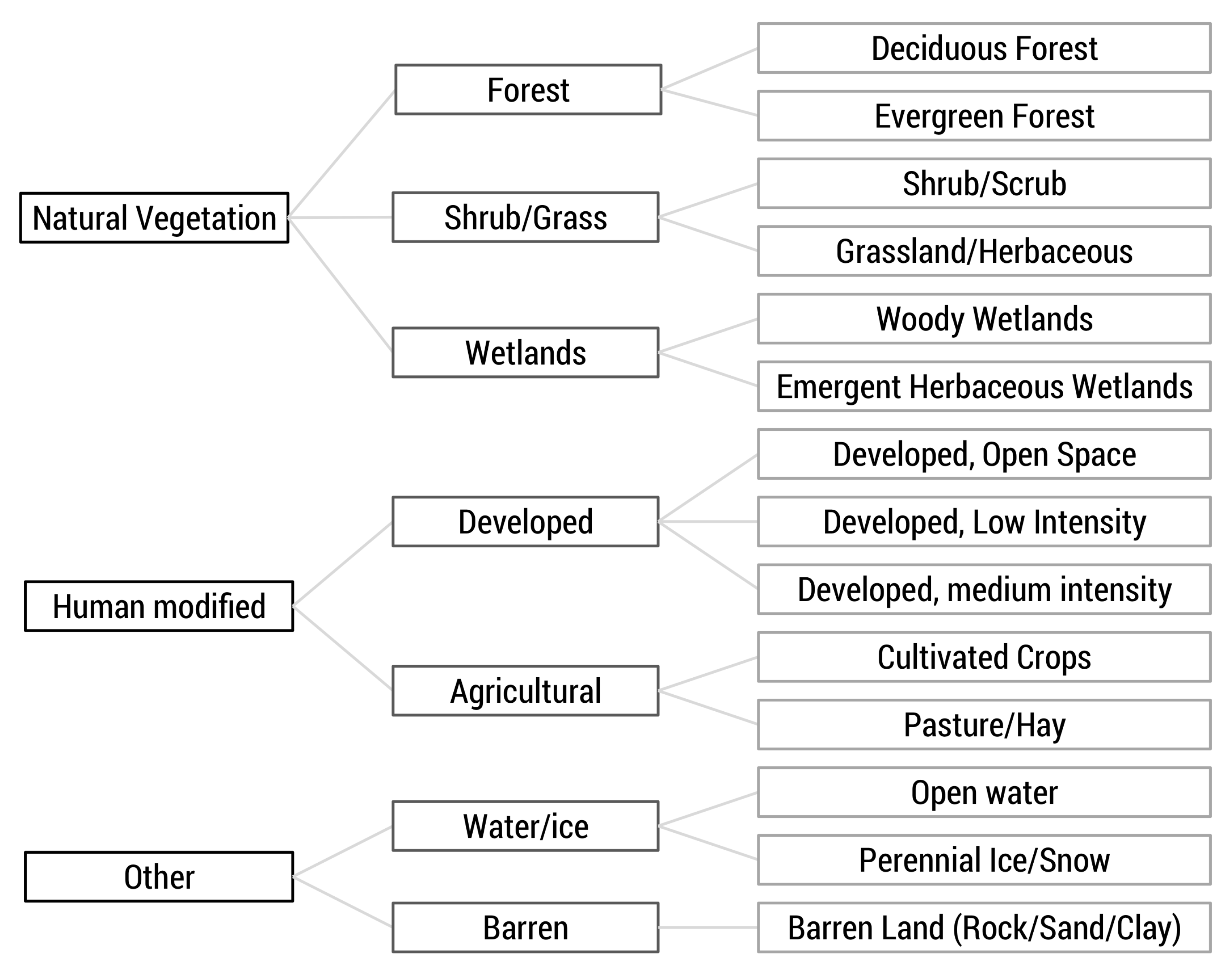
We created our IDU coverage by intersecting the three aforementioned datasets, creating 31,625 polygons. We extracted the average elevation for each IDU and also assigned an elevation class from 1–4, corresponding to 0–1500, 1500–2000, 2000–2500, and >2500 m, respectively, to allow examination of results by elevation band. Although the boundaries between these elevation bands are arbitrary, there are enough IDU polygons within each band to provide meaningful comparisons between elevation bands. Additionally, to aid in analysis and querying we created a three-tiered hierarchy of land cover classification ranging from general (e.g., Natural Vegetation) to more specific (e.g., Evergreen Forest), which was formed by grouping NLCD classifications that are similar (Figure 2).

2.2.2. Hydrological System Model

An extension in Envision called Flow provides flexibility in modeling hydrology and the use of different model representations of hydrological processes. Flow operates on contiguous collections of IDUs that behave in a similar hydrological manner. Each collection of IDUs is referred to as a Hydrologic Response Units (HRUs) [14,32]. We created the HRU coverage by grouping contiguous polygons with identical land cover at the intermediate level (i.e., middle column) level in Figure 2, identical elevation class, and were located in the same HUC-12 catchment. This aggregation process resulted in resulted in 9465 HRUs.

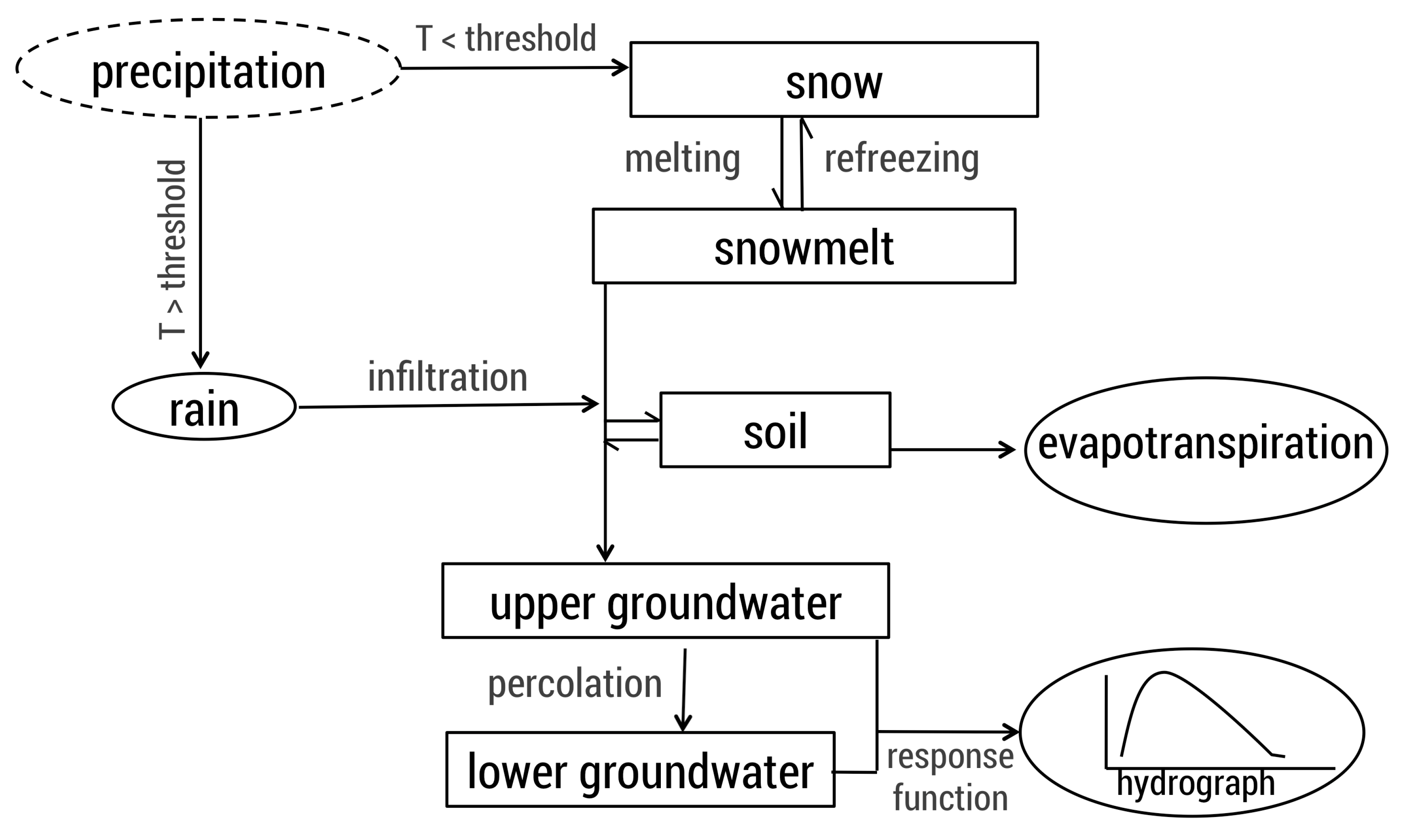
In this study, we used a modified version of the HBV (Hydrologiska Byråns Vattenbalansavdelning) rainfall-runoff model [33] for surface hydrology. HBV is a commonly used conceptual model [34,35,36,37] but has been modified by Envision’s developers to be semi-distributed, operating at the HRU level. Each HRU is conceptualized as a linked reservoir with five layers of storage: snowpack, lakes, soil, upper groundwater, and lower groundwater (Figure 3). Runoff from each HRU is routed to streams using the flowlines associated with the HUC 12 catchments from a modified version of the US National Hydrography Dataset developed by http://www.horizon-systems.com/nhdplus/nhdplusv2_home.php (NHD Plus V2, Table 1). The water balance in each HRU is described by the following equation:

$$P-ET-Q=\frac{d}{dt}\left[SP+SM+UZ+LZ+lakes\right]$$

(1)

where P is precipitation (mm/day), $ET$ is evapotranspiration (mm/day), Q is runoff (mm/day), $SP$ is snow storage (mm), $SM$ is soil moisture storage (mm), $UZ$ is upper groundwater storage (mm), $LZ$ is lower groundwater storage (mm), and $lakes$ refers to lake storage (mm). A more thorough description of the HBV model can be found in other papers [37,38] and a more detailed description of Flow can be found on Envision’s website (http://envision.bioe.orst.edu/).

Evapotranspiration ($ET$) is calculated via a modified Penman-Monteith approach described in the Food and Agriculture Organization’s Irrigation and Drainage paper 56 (FAO56) where a crop coefficient is applied to the $ET$ of a reference plant [39] and was later developed specifically for Idaho [40] using the following equation:

$$ET=E{T}_r·K_c$$

(2)

where $ET$ = evapotranspiration, $E{T}_r$ = reference evapotranspiration (alfalfa, for Idaho), and $K_c$ = crop coefficient.

We used this equation and applied crop coefficient curves that either matched our land cover type directly or estimated crop coefficient curves based upon similarities of crops to land cover types (

Table 2. Land cover type in Envision and the associated crop used to calculate evapotranspiration.

Land Cover	Crop Substituted for Land Cover	Source
Forest	3rd year poplar × 3	Agrimet, Inouye [41]
Shrubland	Sagebrush	Allen and Robison [40]
Grassland	Bunch grass	Allen and Robison [40]
Wetlands	Poplar × 3	Agrimet, Inouye [41]
Developed	Lawn × 0.21	Agrimet, Inouye [41]
Agricultural	Alfalfa (mean)	Agrimet

). Crop coefficients were obtained from AgriMet and [40], with a few modified land cover coefficients from [41].

2.3. Climate Inputs

We used statistically downscaled climate data using the MACA (Multivariate Adaptive Constructed Analogs) method version 1.0 for both historic and future simulations [42]. This data has a spatial resolution of 4 km across the continental U.S. and is available daily for 1950–2100. Downscaled data is available for 20 Global Climate Models (GCMs) from CMIP5 for both Representative Concentration Pathway (RCP) 4.5 and 8.5 scenarios. RCPs are a consistent set of projections that are named according to their additional radiating forcing level at 2100, such that RCP 4.5 equates to +4.5 W/m${}^2$ radiative forcing relative to pre-industrial values by the end of the century [43].

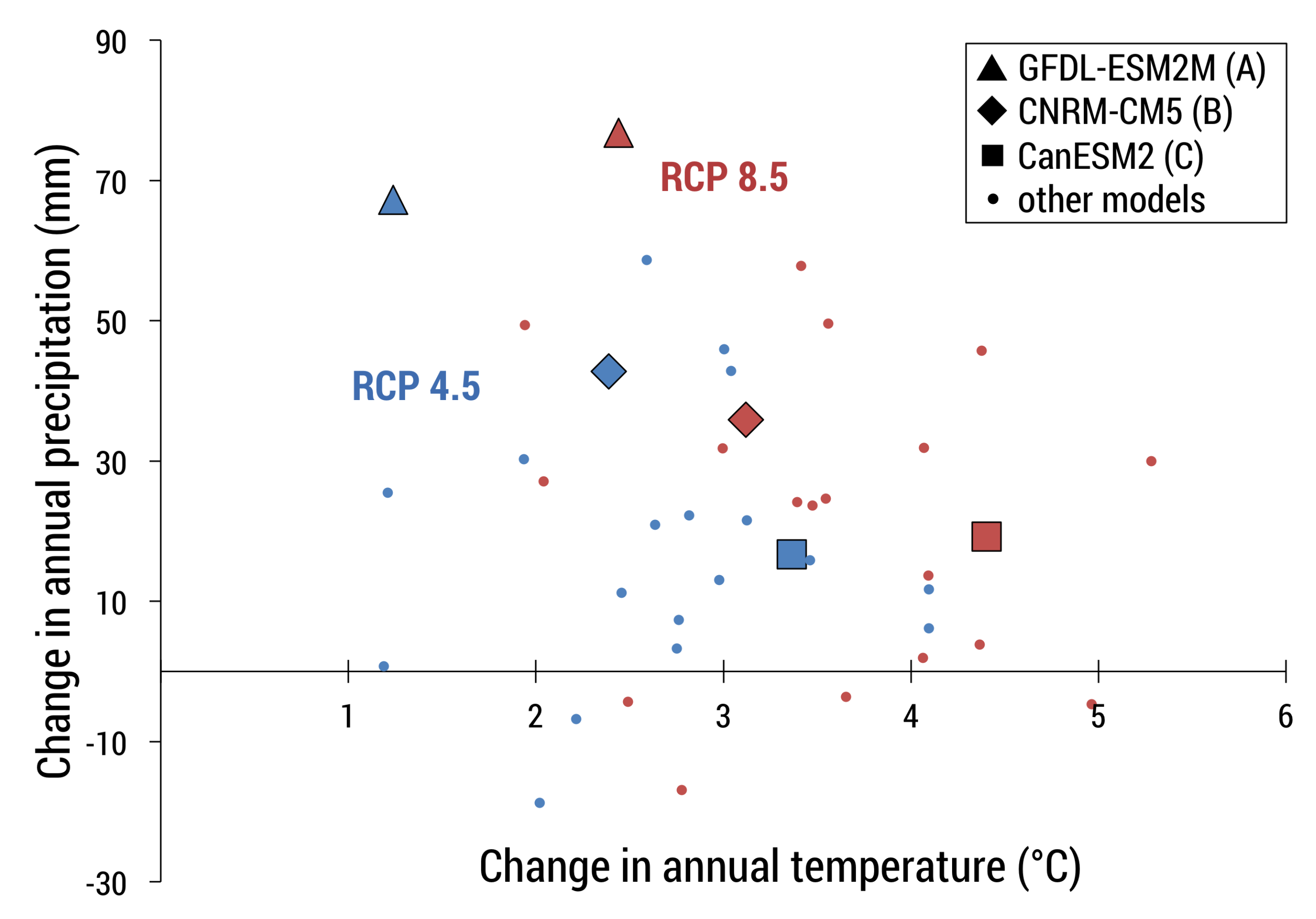
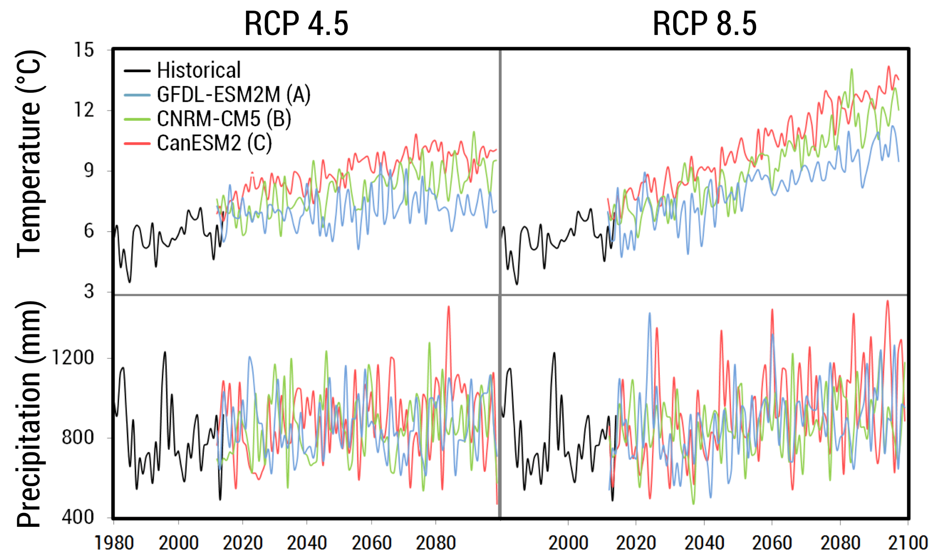
For future simulations, we selected GCMs based upon two criteria. First, we halved our GCM selection to models that performed relatively well when ran over the historical period in the Pacific Northwest region [44], meaning they produced less relative error when compared across several metrics. Secondly, we selected GCMs that captured the range of variability between models as it related to changes in precipitation and temperature (Figure 4). We selected three climate models: CanESM2 (hotter, wetter), CNRM-CM5 (warmer, slightly wetter), and GFDL-ESM2M (less warm, drier), and ran each one for RCP 4.5 and 8.5 scenarios, which resulted in six total simulations of future climate (Figure 5).

Table 3. Naming convention for the six simulations used in this study.

	GFDL-ESM2M	CNRM-CM5	CanESM2
	(Warm)	(Warmer)	(Warmest)
RCP 4.5	A-45	B-45	C-45
RCP 8.5	A-85	B-85	C-85

provides a naming convention for these six simulations to ease in discussing results and implications. For historical simulations from 1980–2014, we used a historical climate dataset, METDATA [45], which was developed using data from the North American Land Data Assimilation System Phase 2 (NLDAS-2) [46] and from the Parameter-elevation Regressions on Independent Slopes Model (PRISM) [20].

The downscaled variables Envision requires for Flow are daily maximum, minimum, and average temperature, precipitation amount, specific humidity, daily downward shortwave radiation, and wind speed. To format the variables for Envision, the following procedure was followed: (1) subset data to the specified region, (2) convert units and rename variables where needed, (3) compute average temperature as the average between minimum and maximum temperature, (4) calculate overall wind speed from the eastward and northward components provided by MACA, and (5) subset into annual files. Scripts created for pre-processing MACA climate data are available online at https://github.com/asteimke/MACA_EnvisionClimate.

2.4. Calibration and Validation

HBV is a semi-conceptual model, and as such, parameters required as input to the model are obtained through calibration because most parameters cannot be physically measured [37]. Numerous combinations of parameter values can yield equally good results (i.e., the equifinality issue) [47,48], which makes it difficult to select the best parameter set. To combat this issue, some studies [41,49] build an objective function to find an adequate parameter set based on the type of information they want to yield from the model (e.g., streamflow volume, timing, snowpack, etc.). Typically, the calibration-validation procedure takes the form of a data-denial experiment. The model is run over a calibration period to select best parameter sets and then re-run over a validation period to ensure that the selected parameter set performs well during this period for which data was not used to calibrate the model.

Fourteen parameters are included within the HBV model and govern rates of exchange between reservoirs. We held five of them constant, while the remaining nine were calibrated. $CFR$ and $CWH$ are insensitive parameters and were held constant as is often done in HBV applications [50]. While many of the parameters are conceptual and cannot be measured, three of them are based on physical properties, so we fixed those parameters to better represent the reality of our study area. We used the Global Gridded Surfaces of Selected Soil Characteristics (IGBP-DIS) dataset [51] and took the average of values for the study area. We used the following datasets from IGBP-DIS: soil field capacity, soil profile available water capacity, and soil wilting point for the parameters $FC$, $LP$, and $WP$, respectively (

Table 4. Parameters for Flow and the ranges/values considered for calibration.

Routine	Parameter	Description	Units	Range	Value
Snow Routine	$TT$	Threshold temperature	${}^{\circ }$C	−0.5–2.0	1.335
	$CFMAX$	Degree-day factor	mm${}^{\circ }$C${}^{-1}$ day${}^{-1}$	1.0–6.0	1.489
	$SFCF$	Snowfall correction factor	-	0.7–1.2	0.568
	$CFR$	Refreeze coefficient	-	-	0.05
	$CWH$	Water holding capacity of snowpack	-	-	0.1
Soil and Evaporation Routine	$FC{}^{*}$	Max depth of water in soil water reservoir	mm	-	399.7
	$LP{}^{*}$	Soil moisture value where actual $ET$ = $PET$	mm	-	247.2
	$WP{}^{*}$	Wilting point in soil for ET to occur	mm	-	156.2
	$BETA$	Shaping coefficient	-	1.0–6.0	2.015
Groundwater and Response Routine	$PERC$	Percolation coefficient	day${}^{-1}$	0.1–2.0	1.272
	$UZL$	Threshold for K0 to outflow	mm	1.0–400.0	365.4
	$K0$	Recession coefficient	day${}^{-1}$	0.1–1.0	0.339
	$K1$	Recession coefficient	day${}^{-1}$	0.01–0.5	0.079
	$K2$	Recession coefficient	day${}^{-1}$	0.001–0.15	0.004

${}^{*}$ values obtained from ORNL DAAC SDAT.

). In each model run, we randomly selected the remaining nine parameters from a uniform distribution between ranges of possible values (Table 4) defined based on previous studies [31,41].

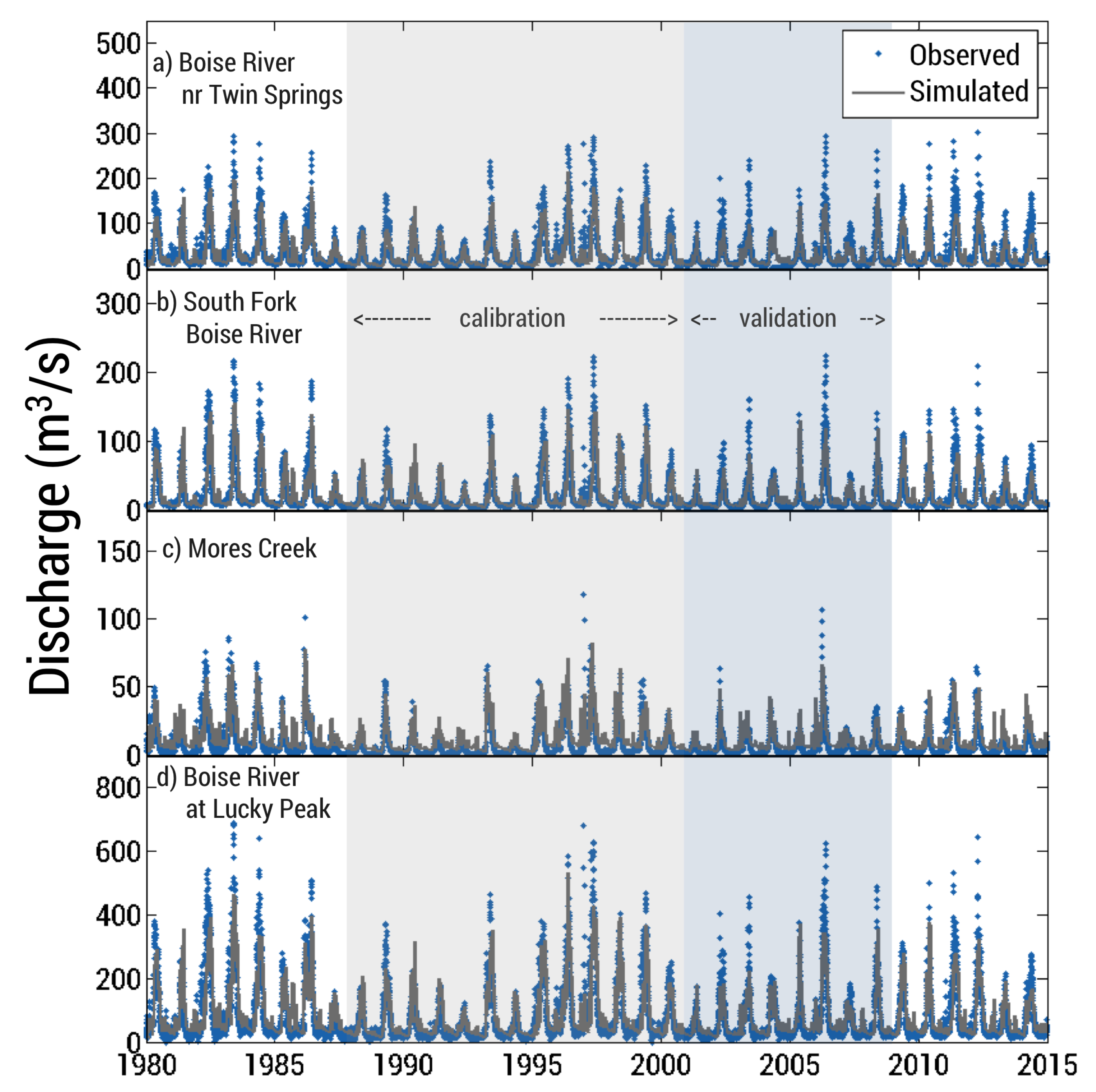
We ran the model for 1000 simulations at a daily time step over the years 1988–2000 (12 years + 1 spin-up year). We selected this time interval for calibration because it encompasses a reasonably long time period and includes both wet and dry years. We compared model output to historical stream discharge records from three long-term USGS gaging stations and snowpack observations from nine SNOTEL (SNOw TELemetry) stations, omitting all leap days from these datasets (

Table 5. Data sites used for calibration and validation. See Figure 1 for locations of gauges.

Type	Name	Drainage Area (km${}^2$)	Record Length	Site ID
Gauge	(a) Boise River nr Twin Springs	2154.9	1911–present	13185000
	(b) SF Boise River nr Featherville	1660.2	1945–present	13186000
	(c) Mores Creek abv Robie Creek	1028.2	1950–present	13200000
	(d) Boise River at Lucky Peak ${}^{*}$	6571	1895–present	LUC
Type	Name	Elevation (m)	Record Length	Site ID
SNOTEL	Atlanta Summit	2310	1981–present	306
	Camas Creek	1740	1992–present	382
	Dollarhide Summit	2566	1981–present	450
	Graham Guard Station	1734	1981–present	496
	Jackson Peak	2155	1981–present	550
	Mores Creek	1859	1981–present	637
	Prairie	1463	1987–present	704
	Trinity	2368	1981–present	830
	Vienna Mine	2731	1979–present	845

${}^{*}$ not an actual gauge, but a calculated daily average of runoff at this location if dams were not present. Obtained from the US Bureau of Reclamation.

). For each run, we calculated the Nash-Sutcliffe Efficiency ($NSE$) [52], $logNSE$, and a volume error ($VE$) using the following equations:

$$NSE=1-\frac{{\sum }_{t=1}^T{\left(Q_{obs}^t-Q_{sim}^t\right)}^2}{{\sum }_{t=1}^T{\left(Q_{obs}^t-\overline{Q_{obs}}\right)}^2}$$

(3)

$$logNSE=1-\frac{{\sum }_{t=1}^T{\left(ln{Q}_{obs}^t-ln{Q}_{sim}^t\right)}^2}{{\sum }_{t=1}^T{\left(ln{Q}_{obs}^t-ln\overline{Q_{obs}}\right)}^2}$$

(4)

$$VE=\frac{{\sum }_{t=1}^t\left(Q_{obs}^t-Q_{sim}^t\right)}{{\sum }_{t=1}^t\left(Q_{obs}^t\right)}$$

(5)

where $Q_{obs}$ is the observed value and $Q_{sim}$ is the simulated value at each daily time step.

$NSE$ coefficients range from $-\infty$ to 1, with 1 indicating a perfect fit of the model to the observed data, and a value of $NSE$ > 0 indicating the model is a better predictor than the historically observed mean. Typically, a model is deemed satisfactory if the $NSE$ is larger than 0.5 [53]. The logarithmic form of the $NSE$ also ranges from $-\infty$ to 1, but is more sensitive to low flow and still reacts to peak flows [54]. The volume error provides insight into whether the model overestimates ($VE$ < 0) or underestimates ($VE$ > 0) total volume, with a value closest to 0 being ideal.

We created an objective function to select the best-performing parameter set and was developed based on work by [41]:

$$Obj=\frac{1}{3}\left(NS{E}_G\right)+\frac{1}{3}\left(logNS{E}_G\right)+\frac{1}{3}\left(NS{E}_S\right)-0.2·\left|V{E}_G\right|$$

(6)

where $NS{E}_G$ is the Nash-Sutcliffe Coefficient of discharge weighted by an areal average of the gauges, $V{E}_G$ is the volume error for the gauges weighted by an areal average, and $NS{E}_S$ is the averaged Nash-Sutcliffe Coefficient for SWE (snow water equivalent) for all SNOTEL sites.

The objective function ideally is as close to 1 as possible, as we wish to maximize $NSE$ and minimize volume bias. The top 1% best performing parameter sets were run over the eight-year validation period (2001–2008) and the set that performed on average the best in both calibration and validation years was chosen for our model. Results of the calibration/validation exercises are reported in the Results section of this manuscript.

2.5. Evaluating Climate Change Impacts

To assess the potential impact of climate change on hydrological regimes, we examined three broad metrics: streamflow, snowpack, and water management. A more detailed description of methods for these metrics is described here.

2.5.1. Streamflow

While Envision has the capability to examine discharge values anywhere along its stream network, we focused here on the aggregation of streamflows for the basin. In all cases, unless mentioned otherwise, streamflow results are for the unregulated discharge on the Boise River occurring at the location of Lucky Peak Dam’s outlet, i.e., the pourpoint of the watershed (Figure 1). This modeled streamflow, as well as daily values for the three major tributaries, can be obtained online [55].

To assess climate change impacts on streamflow, we looked at changes in the amount and timing of discharge. An additional metric we used was the center of timing ($CT$) of streamflow, which is the date when half of the annual volume of water during the water year has arrived at a specified location. We calculated the $CT$ for historical data and future simulations with the following equation [56]:

$$CT=\frac{\sum \left(t_i{Q}_i\right)}{\sum Q_i}$$

(7)

where $t_i$ is the time in days from the start of the water year (1 October) and $Q_i$ is the discharge for that date.

2.5.2. Snowpack

To assess climate impacts on the basin’s snowpack, we looked at averaged values over three elevation zones: low (1500–2000 m), medium (2000–2500 m), and high (2500+ m) zones. These zones cover 43.4%, 25.8%, and 6.9% of the area of interest, respectively. We do not show results for elevations less than 1500 m as the lowest SNOTEL station to aid in calibration is the Prairie site at 1463 m. Within these three zones, we examine the dates and magnitudes of when SWE is at its maximum, as well the April 1 SWE amount. Water managers have historically used the amount of SWE on this date as an indicator for water availability in the upcoming year, as it has correlated well with maximum SWE at many SNOTEL sites in the West historically [57].

2.5.3. Water Management

Since 1986, water managers annually declare a Day of Allocation (DOA) in the Lower Boise River Basin for the purpose of water rights accounting during the irrigation season (April–October). This day is declared on or after the date of maximum reservoir fill and once natural flow is less than irrigation demand (Memo from IDWR Technical Hydrologist Liz Cresto to IDWR Director Gary Spackman, 4 November 2014, Subject: Accounting for the distribution of water to the federal on-stream reservoirs in Water District 63). The DOA occurs after peak runoff and has been shown historically to typically occur once the natural flow of the Boise River at Lucky Peak reaches below 4000 ft${}^3$/s [58], or 113.3 m${}^3$/s (Figure 6), which is roughly equivalent to the diversion demand of the river. It is beneficial for farmers if the DOA occurs later in the season because after the DOA is declared water rights begin to be curtailed, starting with the junior-most water rights holders. While the term DOA is unique to three major river basins in Idaho (i.e., Boise, Payette, and Upper Snake river basins), many western states have similar methods for appropriating water as the irrigation season begins.

To predict how the DOA may change in our modeled scenarios, we assume that diversion rights will continue to be approximately 113.3 m${}^3$/s. We model our DOA date by finding the last day during peak runoff during the irrigation season that flow is greater than 113.3 m${}^3$/s and select the day after. We then manually observe the hydrographs and the DOA selected to ensure we are capturing a date on the downfalling limb of peak runoff and not a later season event. If a later season event was modeled, then we manually select the date on which modeled flow falls below 113.3 m${}^3$/s during the recession limb of spring runoff. We ran the model during the historical period to investigate how well the model reproduces historical DOA using this definition, which provides confidence in our interpretation of DOA changes in modeled future scenarios.

3. Results

3.1. Calibration and Validation

We calibrated and validated the model using historical records from three USGS gauges and nine SNOTEL sites. The parameter set that performed best had an objective function score of 0.63 and 0.62 for calibration and validation periods, respectively (

Table 6. Calibration and validation results for the chosen parameter set for this study.

Calibration					Validation
$NS{E}_G$	$logNS{E}_G$	$V{E}_G$	$NS{E}_S$	$Obj.$	$NS{E}_G$	$logNS{E}_G$	$V{E}_G$	$NS{E}_S$	$Obj.$
0.71	0.61	−0.03	0.59	0.63	0.70	0.66	−0.06	0.52	0.62

). We averaged the $NSE$ for each gauge by its respective drainage area, which resulted in a $NSE$ of 0.71 and 0.70 for calibration and validation, respectively. However, it should be noted that Mores Creek on its own achieved a lesser $NSE$ of 0.58, which is potentially due to this smaller watershed exhibiting some major differences from the other two (notably lower elevation, less precipitation, and less steepness).

Among all gauges, we see relatively good agreement between the model simulations and observed flow for the historic period (Figure 7), although the model frequently under predicts the magnitude of peak flows at all gauge sites and over predicts baseflow at Mores Creek. While the unregulated flow for the Boise River at Lucky Peak (Table 5) was not used to calibrate the model, we used this as an additional verification dataset to ensure accuracy of the model. With the chosen parameter set, we achieved a $NSE$ at this site of 0.74 and $VE$ of −0.01 averaged over the entire calibration and validation period, providing additional confidence in our model.

3.2. Streamflow

3.2.1. Annual Discharge

In all future climate scenarios, we see an increase in the median annual discharge from the Boise River (Figure 8). By midcentury (2040–2069), all climate scenarios showed an increase in annual discharge over historical (1950–2009) averages, with an average increase of 13% and ranges of increase from 6–24%. RCP 8.5 climate scenarios showed a greater rate of increase over RCP 4.5 scenarios. Because our hydrological model did not perform well historically in accurately capturing the magnitude of peak discharges, we do not have adequate confidence to predict future magnitudes in peak or low flows.

3.2.2. Timing of Discharge

While we see some changes in the volume of annual discharge, streamflow is also projected to arrive at significantly different times than in the historical past. However, these arrival times vary greatly between different climate models.

In most future climate scenarios, the date of peak discharge occurs earlier in the season, with an increase in early winter flooding events (Figure 9). In extreme climate cases (i.e., C-85), the average peak discharge occurs approximately 45 days earlier in the period 2040–2060 relative to 1980–2009. In a conservative climate model (i.e., A-45), peak discharge may only be on average about 5 days earlier by midcentury.

To get an understanding of the shift in seasonality and variance between climate scenarios, we can look at the multi-decadal averaged hydrographs between two endmember climate models predicting the least and most amount of change from historical averages (Figure 10). With the coolest climate scenario (A-45), there is little discernible deviation from the historical average hydrograph. However, if we look at the warmest climate scenario (C-85), we see obvious differences in the average hydrograph, where by 2050–2070 the average peak of the hydrograph is over a month and a half earlier. Overall, this warmest scenario shows a shift in seasonality through time, where we see flows occurring earlier in the season with an additional increase in early-season, mid-winter discharge events.

3.2.3. Center of Timing

The historical average (1980–2009) center of timing ($CT$) of streamflow for the UBRB is 22 April. In our simulations, we see this date shift earlier in most of our climate scenarios (Figure 11). Three scenarios (C-45, B-45, and A-85) behave similarly and begin deviating from the historical range of variability between 2040 and 2050, showing a $CT$ date that is 13–17 days earlier on average between 2070 and 2099. Both C-85 and B-85 begin to deviate from historical averages around 2030 and exhibit an average a $CT$ date 27–30 days earlier than the historical average during the 2070–2099 period. A-45 remains relatively similar to historical ranges through the century, although its $CT$ date shifts a few days earlier, resulting in fewer occurrences of exceeding the historical 75th percentile of $CT$ date.

3.3. Snowpack

3.3.1. April 1 SWE

Our results (Figure 12) show a substantial decrease in April 1 SWE in five of the climate scenarios, with lower elevations essentially experiencing no April 1 SWE by midcentury. Higher elevations remain less affected across all RCP 4.5 scenarios but begin substantially decreasing around 2050 in B-85 and C-85 where they experience virtually no April 1 SWE from 2080–2100. Under the A-45 scenario, 1 April SWE experiences variability, but has no discernible downward trend.

3.3.2. Dates and Amounts of Maximum SWE

The previous section suggests that April 1 SWE will, at some point in the future, cease to be a good indicator of maximum SWE. In terms of evaluating potential climate change impacts on SWE in the context of water supply, therefore, it is necessary to examine additional metrics. Specifically, we see the date of maximum SWE happening earlier across most scenarios (Figure 13). Both C-85 and B-85 show maximum SWE occurring more than two months earlier on average by the end of the century. Three scenarios, A-85, C-45, and B-45 behave similarly with maximum SWE date happening between 38 and 42 days earlier than historically observed averages. A-45 produces little change in timing by the end of the century (7 days earlier on average).

The magnitudes of maximum SWE may change as well (Figure 14). Within mid-elevation zones (2000–2500 m), we see a drastic decrease in the occurrence of annual amounts above the historical 75th percentile in five of our climate scenarios. Furthermore, from 2050 onward, we see that 80% (C-85) and 84% (B-85) of the time the maximum SWE is falling below the historical 25th percentile. As with many of the metrics previously mentioned, A-45 shows very little change from historical trends.

3.4. Water Management

Day of Allocation

The developed model reasonably reproduces the DOA in the historical period (R${}^2$ = 0.90), although it over-predicted the date on average 4.8 days later (Figure 6). Thus, the defined metric for the DOA provides a reasonably robust vehicle to analyze how the DOA may shift under different climate scenarios. Our results show the DOA occurring much earlier under four of our scenarios (Figure 15), ranging from 11 to 33 days earlier on average by the end of the century. Scenarios A-45 and B-45 resulted in little to no change in the trend of DOA. While the DOA remains variable on an interannual basis, we do not see significant changes in variability of DOA through time (

Table 7. Simulated mean Day of Allocation (DOA) and standard deviation (italicized, in parentheses) over three future time intervals. Historical (1986–2014) average DOA is 6/19.

Time Period	A-45	B-45	C-45	A-85	B-85	C-85
2010–2039	6/22 (12.0)	6/21 (20.0)	6/10 (24.3)	6/19 (17.1)	6/20 (20.6)	6/10 (19.0)
2040–2069	6/20 (17.3)	6/20 (15.3)	6/7 (16.8)	6/15 (13.1)	6/15 (17.2)	5/30 (23.5)
2070–2099	6/23 (15.1)	6/18 (16.1)	5/29 (24.0)	6/8 (14.9)	5/27 (25.6)	5/17 (23.5)

).

4. Discussion

4.1. Trends in Future Hydrological Regimes

We calibrated our model using metrics that included historic snowpack levels, daily streamflow, logarithmic transformation of streamflow, and streamflow volume. Choosing multiple metrics to select the best parameter set provides some additional confidence that the model is simulating key attributes of historical hydrological regimes and, therefore, strengthens confidence in the robustness of our interpretations of future climate change impacts on hydrological regimes predicted by the model.

We have shown that a variety of hydrological regime characteristics within the UBRB could exhibit significant changes, depending on which climate model and RCP scenario is used. However, certain trends are consistent across several considered climate scenarios and are consistent with other projections [13,16,41]. Our results suggest an increase in annual water discharge, but with significantly altered timing, with flows arriving much earlier than historically. Our modeled results also show a decrease in the total amount of snowpack, an earlier melting date, and earlier dates of peak snowpack. In order to reconcile how annual discharge can increase while the snowpack is consistently smaller in volume and more ephemeral in time, we examined the seasonality of the precipitation input to the model. This allows us to better understand whether observed changes in discharge volume are primarily related to changes in the seasonality of input precipitation, changes in the seasonal dynamics of snowpacks, or some combination of both. Typically, however, the precipitation exhibits increases across all seasons rather than large shifts between seasons in precipitation. Accordingly, this may indicate that the basin could begin transitioning from being snowmelt-dominated to a regime that is mixed rain- and snow-dominated watershed moving forward.

4.2. Management Implications

Our modeled scenarios support previous studies [59,60] that April 1 SWE is not likely to remain a reliable metric for estimating maximum SWE (and therefore snow water storage) in the future for water resource prediction and management. This work suggests declines in the amount of SWE on April 1 and a maximum SWE date over a month earlier than historically observed in five of the six simulations. Rather than choosing a static date to estimate peak SWE across a vast region, managers may need to more closely monitor the relationship between hydrological regimes and the timing of peak SWE in their regions, potentially necessitating increased investment in monitoring and modeling of snow conditions.

There is little evidence to conclude that we will experience future water shortages from the UBRB in an absolute sense, as most models suggest at least a small increase in annual discharge. However, we will likely experience hydrological shifts that are outside of our current range of variability. All climate scenarios show peak discharge occurring earlier in the year. This is problematic for reservoir managers who primarily manage dams to provide storage for flood mitigation. Managers might have to release more ’usable’ water from reservoirs in preparation for these events, which potentially could equate to shortages later in the irrigation season. Such outcomes could be viewed as an "operational deficit" that arises because of a mismatch between the release of water from storage for flood mitigation and the timing of water allocation as codified in water rights laws.

At the same time, in this region agricultural land is increasingly transitioning to urban areas [61], which could indicate that future water demand may be substantially different from the past. With warmer climates, farmers might plant earlier in the season, which would change the timing of water demand. Recent modeling efforts have shown that current water rights are not always able to support irrigation demand [31,62]. Agricultural water use efficiency, however, is likely to increase with technological advances like genetically modified crops, which could change spatiotemporal patterns of water demand. A more comprehensive examination of how, when, and where water is being used downstream and how that may change in the future will help managers understand to what extent regional water infrastructure is vulnerable and the potential policies that might help to mitigate effects.

Our results show that under most climate scenarios, the Day of Allocation occurs much earlier than it has historically, with two models showing the date moving by over a month earlier. If this projection becomes reality, then there is an earnest need for exploring potential conflicts between water users in the future as curtailments may come increasingly early and impact more water rights holders than in previous decades. It may be necessary, for instance, to incentivize farmers to transition to more efficient irrigation practices (e.g., switching from flood to drip irrigation) and to diversify with crops that require less water, or expand other solutions like water banking and water markets. If junior water rights holders are curtailed over a month earlier without any mitigation practices set in place, it may result in substantial repercussions to Idaho’s agricultural sector. These effects are compounded if other mountain water supply basins exhibit similar changes to hydrological regimes.

4.3. Study Limitations

It is worth noting that this study did not simulate reservoir operations. There are three dams present in the study area that are located close to the outlet of the basin. For purposes of simplicity, the present work focuses on evaluating the ramifications of climate change on natural flows in the UBRB and capturing reservoir operations is outside the scope of this study. A significant challenge in future work will arise from the need to develop plausible scenarios by which water managers from federal agencies, irrigation districts, environmental groups, and utility companies can create strategies to adapt to potential changes in hydrological regimes similar to those simulated here. Given the complexities in both biophysical and social responses to climate change, such studies will likely need to be region- and context-specific.

An additional source of uncertainty in this study lies in the land cover data used in the hydrological model, which was treated as static. Specifically, the land cover dataset used represents a snapshot estimated based on Landsat reflectances from 2011. Vegetation along ecotones is sensitive to changes in climate, and there are likely to be additional large-scale vegetation and land cover changes that occur after wildfire events or through land management actions. Future modeling studies should incorporate plausible shifts in vegetation to understand the sensitivity of changes in hydrological regimes to associated changes in land cover as well as climate change. This might be best accomplished using a physically-based model, rather than the conceptual model used in this study, to be able to better capture complex interactions between climate, hydrology, vegetation dynamics, and changing land cover.

5. Conclusions

In this study, we used an integrated modeling framework, Envision, to simulate future hydrology in a mountainous watershed that supports an urban and agriculturally intensive region below it. We calibrated the hydrological model to metrics of both streamflow and snowpack, and it performed well under historical conditions. We ran the model to the year 2100 under six alternative simulations (three GCMs and two RCP scenarios) to analyze future possible hydrological regimes, focusing primarily on the timing and magnitude of the accumulation, retention, and release of water from seasonal snowpacks and the associated streamflow.

Our results suggest that overall annual streamflow will increase, and five of six simulations suggest hydrological regimes that will deliver runoff substantially earlier than historically observed. This could lead to operational water shortages later in the season as water managers balance release of water from storage in reservoirs to mitigate flooding hazards with retention of water for supplying irrigation in the warm, dry summers. Without changes in existing policies, these hydrological regimes could have repercussions to late-season irrigation demand, hydropower operations, recreational flows, and municipal water supply.

Mountainous, snowmelt-dominated watersheds have already begun responding to climate change, which will almost certainly continue in the future. The degree to which the runoff response of these watersheds changes in association with climate change is uncertain, and will depend heavily on the nature of the change in the climatic forcing variables. Increasingly sophisticated comparisons with climate model predictions and observations, as well as regionally focused and contextual modeling of coupled hydrological and social systems, will improve our ability to constrain how hydrological regimes will change in the future. This may increase the efficacy of efforts to respond to changes and potential conflicts between potentially competing demands for water.

References

1. Mote, P.W.; Hamlet, A.F.; Clark, M.P.; Lettenmaier, D.P. Declining mountain snowpack in Western North America. Bull. Am. Meteorol. Soc. 2005, 86, 39–50. [Google Scholar] [CrossRef]
2. Regonda, S.K.; Rajagopalan, B.; Clark, M.; Pitlick, J. Seasonal cycle shifts in hydroclimatology over the Western United States. J. Clim. 2005, 18, 372–384. [Google Scholar] [CrossRef]
3. Knowles, N.; Dettinger, M.D.; Cayan, D.R. Trends in snowfall versus rainfall in the Western United States. J. Clim. 2006, 19, 4545–4559. [Google Scholar] [CrossRef]
4. Haddeland, I.; Heinke, J.; Biemans, H.; Eisner, S.; Flörke, M.; Hanasaki, N.; Konzmann, M.; Ludwig, F.; Masaki, Y.; Schewe, J.; et al. Global water resources affected by human interventions and climate change. Proc. Natl. Acad. Sci. USA 2014, 111, 3251–3256. [Google Scholar] [CrossRef] [PubMed]
5. Deb, P.; Babel, M.S.; Denis, A.F. Multi-GCMs approach for assessing climate change impact on water resources in Thailand. Model. Earth Syst. Environ. 2018, 4, 825–839. [Google Scholar] [CrossRef]
6. Barnett, T.P.; Adam, J.C.; Lettenmaier, D.P. Potential impacts of a warming climate on water availability in snow-dominated regions. Nature 2005, 438, 303–309. [Google Scholar] [CrossRef] [PubMed]
7. Li, D.; Wrzesien, M.L.; Durand, M.; Adam, J.; Lettenmaier, D.P. How much runoff originates as snow in the western United States, and how will that change in the future? Geophys. Res. Lett. 2017, 44, 6163–6172. [Google Scholar] [CrossRef]
8. Huntington, T.G. Evidence for intensification of the global water cycle: Review and synthesis. J. Hydrol. 2006, 319, 83–95. [Google Scholar] [CrossRef]
9. Turral, H.; Burke, J.J.; Faurès, J.M. Climate Change, Water and Food Security; Food and Agriculture Organization of the United Nations: Rome, Italy, 2011. [Google Scholar]
10. Oki, T. Global hydrological cycles and world water resources. Science 2006, 313, 1068–1072. [Google Scholar] [CrossRef] [PubMed]
11. Schewe, J.; Heinke, J.; Gerten, D.; Haddeland, I.; Arnell, N.W.; Clark, D.B.; Dankers, R.; Eisner, S.; Fekete, B.M.; Colón-González, F.J.; et al. Multimodel assessment of water scarcity under climate change. Proc. Natl. Acad. Sci. USA 2014, 111, 3245–3250. [Google Scholar] [CrossRef] [PubMed] [Green Version]
12. Markoff, M.S.; Cullen, A.C. Impact of climate change on Pacific Northwest hydropower. Clim. Chang. 2008, 87, 451–469. [Google Scholar] [CrossRef]
13. Adam, J.C.; Hamlet, A.F.; Lettenmaier, D.P. Implications of global climate change for snowmelt hydrology in the twenty-first century. Hydrol. Process. 2009, 23, 962–972. [Google Scholar] [CrossRef]
14. Jin, X.; Sridhar, V. Impacts of climate change on hydrology and water resources in the Boise and Spokane River Basins. JAWRA J. Am. Water Resour. Assoc. 2011, 48, 197–220. [Google Scholar] [CrossRef]
15. Ficklin, D.L.; Stewart, I.T.; Maurer, E.P. Climate change impacts on streamflow and subbasin-scale hydrology in the Upper Colorado River Basin. PLoS ONE 2013, 8, e71297. [Google Scholar] [CrossRef] [PubMed]
16. Gergel, D.R.; Nijssen, B.; Abatzoglou, J.T.; Lettenmaier, D.P.; Stumbaugh, M.R. Effects of climate change on snowpack and fire potential in the western USA. Clim. Chang. 2017, 141, 287–299. [Google Scholar] [CrossRef]
17. Vicuna, S.; Maurer, E.P.; Joyce, B.; Dracup, J.A.; Purkey, D. The sensitivity of California water resources to climate change scenarios. JAWRA J. Am. Water Resour. Assoc. 2007, 43, 482–498. [Google Scholar] [CrossRef]
18. Stewart, I.T. Changes in snowpack and snowmelt runoff for key mountain regions. Hydrol. Process. 2009, 23, 78–94. [Google Scholar] [CrossRef]
19. Palmer, M.A.; Reidy Liermann, C.A.; Nilsson, C.; Flörke, M.; Alcamo, J.; Lake, P.S.; Bond, N. Climate change and the world’s river basins: Anticipating management options. Front. Ecol. Environ. 2008, 6, 81–89. [Google Scholar] [CrossRef]
20. Daly, C.; Halbleib, M.; Smith, J.I.; Gibson, W.P.; Doggett, M.K.; Taylor, G.H.; Curtis, J.; Pasteris, P.P. Physiographically sensitive mapping of climatological temperature and precipitation across the conterminous United States. Int. J. Climatol. 2008, 28, 2031–2064. [Google Scholar] [CrossRef] [Green Version]
21. Isaak, D.J.; Luce, C.H.; Rieman, B.E.; Nagel, D.E.; Peterson, E.E.; Horan, D.L.; Parkes, S.; Chandler, G.L. Effects of climate change and wildfire on stream temperatures and salmonid thermal habitat in a mountain river network. Ecol. Appl. 2010, 20, 1350–1371. [Google Scholar] [CrossRef] [PubMed] [Green Version]
22. Clark, G.M. Changes in patterns of streamflow from unregulated watersheds in Idaho, Western Wyoming, and Northern Nevada. JAWRA J. Am. Water Resour. Assoc. 2010, 46, 486–497. [Google Scholar] [CrossRef]
23. Kunkel, K.E. Temporal variations in frost-free season in the United States: 1895–2000. Geophys. Res. Lett. 2004, 31, 399. [Google Scholar] [CrossRef]
24. Kormos, P.R.; Luce, C.H.; Wenger, S.J.; Berghuijs, W.R. Trends and sensitivities of low streamflow extremes to discharge timing and magnitude in Pacific Northwest mountain streams. Water Resour. Res. 2016, 52, 4990–5007. [Google Scholar] [CrossRef] [Green Version]
25. Stillwater, L. The Effects of Climate Change on the Operation of Boise River Reservoirs, Initial Assessment Report; United States Bureau of Reclamation, Department of the Interior: Boise, ID, USA, 2008. [Google Scholar]
26. Taylor, K.E.; Stouffer, R.J.; Meehl, G.A. An overview of CMIP5 and the experiment design. Bull. Am. Meteorol. Soc. 2012, 93, 485–498. [Google Scholar] [CrossRef]
27. Bolte, J.P.; Hulse, D.W.; Gregory, S.V.; Smith, C. Modeling biocomplexity – actors, landscapes and alternative futures. Environ. Model. Softw. 2007, 22, 570–579. [Google Scholar] [CrossRef] [Green Version]
28. Wu, H.; Bolte, J.P.; Hulse, D.; Johnson, B.R. A scenario-based approach to integrating flow-ecology research with watershed development planning. Geodes. Chang. World Chang. Des. 2015, 144, 74–89. [Google Scholar] [CrossRef]
29. Turner, D.P.; Conklin, D.R.; Bolte, J.P. Projected climate change impacts on forest land cover and land use over the Willamette River Basin, Oregon, USA. Clim. Chang. 2015, 133, 335–348. [Google Scholar] [CrossRef]
30. Hulse, D.; Branscomb, A.; Enright, C.; Johnson, B.; Evers, C.; Bolte, J.; Ager, A. Anticipating surprise: Using agent-based alternative futures simulation modeling to identify and map surprising fires in the Willamette Valley, Oregon USA. Geodes. Chang. World Chang. Des. 2016, 156, 26–43. [Google Scholar] [CrossRef]
31. Han, B.; Benner, S.G.; Bolte, J.P.; Vache, K.B.; Flores, A.N. Coupling biophysical processes and water rights to simulate spatially distributed water use in an intensively managed hydrologic system. Hydrol. Earth Syst. Sci. 2017, 21, 3671–3685. [Google Scholar] [CrossRef] [Green Version]
32. Turner, D.P.; Conklin, D.R.; Vache, K.B.; Schwartz, C.; Nolin, A.W.; Chang, H.; Watson, E.; Bolte, J.P. Assessing mechanisms of climate change impact on the upland forest water balance of the Willamette River Basin, Oregon. Ecohydrology 2016, 10, e1776. [Google Scholar] [CrossRef]
33. Bergström, S. Development and Application of a Conceptual Runoff Model for Scandinavian Catchments. Technical Report RH07, Norrköping. 1976. Available online: http://www.citeulike.org/group/14742/article/8861475 (accessed on 19 October 2018).
34. Seibert, J. Multi-criteria calibration of a conceptual runoff model using a genetic algorithm. Hydrol. Earth Syst. Sci. 2000, 4, 215–224. [Google Scholar] [CrossRef] [Green Version]
35. Woodsmith, R.; Vache, K.; McDonnell, J.; Seibert, J.; Helvey, J. The entiat experimental forest: A unique opportunity to examine hydrologic response to wildfire. In Proceedings of the Forest Service National Earth Sciences Conference, Advancing the Fundamental Sciences, San Diego, CA, USA, 18–22 October 2004; PNW-GTR-689. Furniss, M., Clifton, C., Ronnenbery, K., Eds.; USDA, Forest Service: Portland, OR, USA, 2007; pp. 205–216. [Google Scholar]
36. Abebe, N.A.; Ogden, F.L.; Pradhan, N.R. Sensitivity and uncertainty analysis of the conceptual HBV rainfall–runoff model: Implications for parameter estimation. J. Hydrol. 2010, 389, 301–310. [Google Scholar] [CrossRef]
37. Bergström, S.; Lindström, G. Interpretation of runoff processes in hydrological modelling-experience from the HBV approach. Hydrol. Process. 2015, 29, 3535–3545. [Google Scholar] [CrossRef]
38. Seibert, J. Regionalisation of parameters for a conceptual rainfall-runoff model. Agric. For. Meteorol. 1999, 98–99, 279–293. [Google Scholar] [CrossRef]
39. Allen, R.G.; Pereira, L.S.; Raes, D.; Smith, M. Crop Evapotranspiration–Guidelines for Computing Crop Water Requirements; Technical Report 56; FAO Irrigation and Drainage Paper; FAO: Rome, Italy, 1998. [Google Scholar]
40. Allen, R.G.; Robison, C.W. Evapotranspiration and consumptive irrigation water requirements for Idaho. In Precipitation Deficit Table for Boise WSFO Airport; University of Idaho: Moscow, ID, USA, 2007. [Google Scholar]
41. Inouye, A.M. Development of a Hydrologic Model to Explore Impacts of Climate Change on Water Resources in the Big Wood Basin, Idaho. Master’s Thesis, Oregon State University, Corvallis, OR, USA, 2014. [Google Scholar]
42. Abatzoglou, J.T.; Brown, T.J. A comparison of statistical downscaling methods suited for wildfire applications. Int. J. Climatol. 2011, 32, 772–780. [Google Scholar] [CrossRef] [Green Version]
43. Van Vuuren, D.P.; Edmonds, J.; Kainuma, M.; Riahi, K.; Thomson, A.; Hibbard, K.; Hurtt, G.C.; Kram, T.; Krey, V.; Lamarque, J.F.; et al. The representative concentration pathways: An overview. Clim. Chang. 2011, 109, 5. [Google Scholar] [CrossRef]
44. Rupp, D.E.; Abatzoglou, J.T.; Hegewisch, K.C.; Mote, P.W. Evaluation of CMIP5 20th century climate simulations for the Pacific Northwest USA. J. Geophys. Res. Atmos. 2013, 118, 10884–10906. [Google Scholar] [CrossRef]
45. Abatzoglou, J.T. Development of gridded surface meteorological data for ecological applications and modelling. Int. J. Climatol. 2011, 33, 121–131. [Google Scholar] [CrossRef] [Green Version]
46. Mitchell, K.E. The multi-institution North American Land Data Assimilation System (NLDAS): Utilizing multiple GCIP products and partners in a continental distributed hydrological modeling system. J. Geophys. Res. 2004, 109, 7449. [Google Scholar] [CrossRef]
47. Beven, K. A manifesto for the equifinality thesis. J. Hydrol. 2006, 320, 18–36. [Google Scholar] [CrossRef] [Green Version]
48. Gupta, H.V.; Beven, K.J.; Wagener, T. Model calibration and uncertainty estimation. Encycl. Hydrol. Sci. 2005. [Google Scholar] [CrossRef]
49. Madsen, H. Parameter estimation in distributed hydrological catchment modelling using automatic calibration with multiple objectives. Snow Atmos. Interact. Hydrol. Conseq. 2003, 26, 205–216. [Google Scholar] [CrossRef]
50. Seibert, J. Estimation of parameter uncertainty in the HBV model: Paper presented at the Nordic Hydrological Conference (Akureyri, Iceland-August 1996). Hydrol. Res. 1997, 28, 247–262. [Google Scholar] [CrossRef]
51. Hope, A.; Peck, E.L. Soil Moisture Release Data (FIFE); ORNL DAAC: Oak Ridge, TN, USA, 1994. [Google Scholar]
52. Nash, J.E.; Sutcliffe, J.V. River flow forecasting through conceptual models part I—A discussion of principles. J. Hydrol. 1970, 10, 282–290. [Google Scholar] [CrossRef]
53. Moriasi, D.N.; Arnold, J.G.; Van Liew, M.W.; Bingner, R.L.; Harmel, R.D.; Veith, T.L. Model evaluation guidelines for systematic quantification of accuracy in watershed simulations. Trans. ASABE 2007, 50, 885. [Google Scholar] [CrossRef]
54. Krause, P.; Boyle, D.P.; Bäse, F. Comparison of different efficiency criteria for hydrological model assessment. Adv. Geosci. 2005, 5, 89–97. [Google Scholar] [CrossRef]
55. Steimke, A.; Flores, A.; Han, B.; Brandt, J.; Som-Castellano, R. Modeled Impacts of Climate Change on Regional Hydrology in the Upper Boise River Basin, Idaho. 2017. Available online: https://scholarworks.boisestate.edu/leaf_data/1/ (accessed on 19 October 2018).
56. Stewart, I.T.; Cayan, D.R.; Dettinger, M.D. Changes toward earlier streamflow timing across Western North America. J. Clim. 2005, 18, 1136–1155. [Google Scholar] [CrossRef]
57. Bohr, G.S.; Aguado, E. Use of April 1 SWE measurements as estimates of peak seasonal snowpack and total cold-season precipitation. Water Resour. Res. 2001, 37, 51–60. [Google Scholar] [CrossRef] [Green Version]
58. Garst, R.D. Using Mountain Snowpack to Predict Summer Water Availability in Semiarid Mountain Watersheds. Master’s Thesis, Boise State University, Boise, ID, USA, 2017. [Google Scholar]
59. Pederson, G.T.; Gray, S.T.; Woodhouse, C.A.; Betancourt, J.L.; Fagre, D.B.; Littell, J.S.; Watson, E.; Luckman, B.H.; Graumlich, L.J. The unusual nature of recent snowpack declines in the North American Cordillera. Science 2011, 333, 332–335. [Google Scholar] [CrossRef] [PubMed]
60. Klos, P.Z.; Link, T.E.; Abatzoglou, J.T. Extent of the rain-snow transition zone in the western U.S. under historic and projected climate. Geophys. Res. Lett. 2014, 41, 4560–4568. [Google Scholar] [CrossRef] [Green Version]
61. Dahal, K.R.; Benner, S.; Lindquist, E. Urban hypotheses and spatiotemporal characterization of urban growth in the Treasure Valley of Idaho, USA. Appl. Geogr. 2017, 79, 11–25. [Google Scholar] [CrossRef]
62. Deb, P.; Shrestha, S.; Babel, M.S. Forecasting climate change impacts and evaluation of adaptation options for maize cropping in the hilly terrain of Himalayas: Sikkim, India. Theor. Appl. Climatol. 2015, 121, 649–667. [Google Scholar] [CrossRef]
Figure 1. Overview of the study area with major land cover types and locations of SNOTEL stations and gauge locations.
Water 10 01490 g001
Figure 2. Land use/land cover tree developed for Envision. The tree allows for modeling algorithms to be applied at different hierarchy levels, from more general to more specific land types. The finest categories on the right correspond to the NLCD land classification system.
Water 10 01490 g002
Figure 3. Flowchart of the different hydrological processes and reservoirs within the Flow model in Envision, modified from [31].
Water 10 01490 g003
Figure 4. Change in climate variables from 1979–2000 to 2040–2069 for MACA downscaled GCMs [42]. Blue and red points represent RCP 4.5 and 8.5 scenarios, respectively. The larger icons represent the GCMs selected for this study.
Water 10 01490 g004
Figure 5. Temporal projections for annual mean temperature and precipitation for the six simulations used in this study. Temperature increases in all scenarios, but precipitation is more variable.
Water 10 01490 g005
Figure 6. (a) Relationship between the day natural flow at Lucky Peak reaches below 4000 ft 3 /s and the date the Day of Allocation is declared, modified from [58]. (b) Our modeled historical Day of Allocation using the same method as (a). Dashed line is 1:1 in both plots.
Water 10 01490 g006
Figure 7. Observed and simulated streamflows during the historical period from 1980 to 2014. See Figure 1 for locations of sites. The model does a good job at simulating historical flows, but under estimates magnitude of peak flows and over estimates baseflow at Mores Creek.
Water 10 01490 g007
Figure 8. Average annual discharge of the UBRB. Values for 1980–2009 are observed. In most scenarios, we see an increase in overall discharge throughout the century. Boxes represent upper and lower quartiles and lines inside are the median.
Water 10 01490 g008
Figure 9. Date when peak discharge occurs for the Boise River at Lucky Peak. Values for 1980–2009 are observed. Overall, we see peak discharge date moving substantially earlier in five scenarios.
Water 10 01490 g009
Figure 10. Hydrographs averaged over 2-decadal timespans for scenarios predicting the least amount of change (A-45) and the greatest amount of change (C-85) from historical.
Water 10 01490 g010
Figure 11. Center of timing of streamflow for historic and future simulations. Dashed lines show the upper and lower quartile ranges from 1980–2009.
Water 10 01490 g011
Figure 12. 10-year moving average percentage of April 1 SWE from historical simulated averages (1980-2009) for low, medium, and high elevation zones, corresponding to 1500–2000, 2000–2500, and 2500+ m, respectively.
Water 10 01490 g012
Figure 13. 10-year moving average of dates of maximum SWE for three elevation zones. Values for 1980–2009 are simulated with MACA METDATA.
Water 10 01490 g013
Figure 14. Maximum SWE amount (mm) for mid-elevations (2000–2500 m). Values for 1980–2009 are simulated with MACA METDATA. Dashed lines show upper and lower quartile ranges for 1980–2009.
Water 10 01490 g014
Figure 15. Simulated future (2010–2099) and historical (1986–2014) Day of Allocation with a 7-year moving average. Shaded area is ± 0.5 σ of 7-year moving average values.
Water 10 01490 g015