Prediction of Water Utility Performance: The Case of the Water Efficiency Rate

Abstract

This paper deals with the development of a decision-aiding model for predicting, in an ex-ante way, the effects of a mix of actions on an asset and on its operation. The objective is then to define a compromised policy between costs and performance improvements. We investigate the use of multiple regression analysis (MRA) and an artificial neural network (ANN) to establish causal relationships between the network efficiency rate, and a set of explanatory variables on one hand, and potential water loss management actions such as leak detection, maintenance and asset renewal, on the other hand. The originality of our approach is in developing a two-step ex-ante model for predicting the efficiency rate involving low and high level explanatory variables in a context of unavailability of data at the scale of the water utility. The first step exploits a national French database «SISPEA» (Système d’Information d’information sur les Services Publics d’Eau et d’Assainissement) to calibrate a general prediction model that establishes a correlation between efficiency (output) and other performance indicators (inputs). The second step involves the utility manager to build a causal model between endogenous and exogenous variables of a specific water network (low level) and performance indicators considered as inputs for the previous step (high level). Uncertainty is taken into account by Monte Carlo simulations. An application of our decision model on a water utility in the southeast of France is provided as a case study.

1. Introduction

Previous water network management experiences suggest that water loss management actions may influence performance in various ways. As much as one important challenge of our work is to identify the most relevant actions that significantly enhance performance in terms of water loss [1], our work also aims to explain relationships between actions and their consequences. Non-Revenue Water (NRW) and water loss reduction are one of the most important challenges for water utilities in terms of economy of energy, loss of revenue, safety and environmental issues [2].

In France, about 20% of produced water is not delivered [3]. We assume that relevant actions to improve leakage water ratio are the following: pressure regulation, leak detection, maintenance, asset renewal and metering accuracy. The problem of leakage management and how it could be improved through the adoption of data analytics techniques and hydraulic simulation is discussed in [4]. The problem of metering-error is addressed in [5] by developing an integrated model based on International Water Association (IWA) water balance audit and genetic algorithm.

The literature review shows that the use of machine learning and multiple regression analysis (MRA) seems relevant for predicting network efficiency rate or water loss. In the domain of water networks, Artificial Neural Network (ANN) and MRA are widely used for solving prediction problems. Several input parameters from more than three hundred Districts Meter areas (DMA) to estimate the non-revenue water (NRW) using MRA and ANN models can be considered as shown in [6].

The authors conclude that ANN seems to be more accurate than standard statistical methods, as with MRA. The accuracy of estimation depends on the number of ANN’s neurons. An estimation of the leakage ratio based on 6 effective parameters by combining ANN with Principal Component Analysis (PCA) is carried out in [7]. PCA-ANN multiple hidden layers seem more accurate than standard ANN. A comparison of the performance of ANN and support vector regression (SVR) in predicting the pipe burst rate (PBR) is made in [8]. ANN was applied on multiple years of data collection from pipes in order to predict water mains failure; data availability seems a prerequisite for prediction accuracy [9]. The authors test six ANN models in order to select the best configuration for failures prediction to elaborate rehabilitation strategies of water distribution systems. For the same problem, a model is developed for more accurate prediction for pipes failures based on ANN and neuro-fuzzy systems [10]. The authors compare the ANN model with conventional multivariate regression, and conclude that the ANN is more accurate for prediction. An ANN model to forecast pipe breaks involving multiple explanatory variables including pipe age, diameter, length, and surrounding soil type can be created as shown in [11]. The authors build a decision model based on historical data provided by the water utility of Kingston in Canada. ANN multilayer perceptron (MLP) is used to predict the frequency of water mains failure based on 11 input data (production, consumption, and water losses, sale, number of water-meters, length and number of failures of water mains, distribution pipes and house connections) [12]. The neural network was trained on six years of historical data. On a similar topic, a method for discerning sections of water networks in need of renewal is presented in [13]. They aim to develop a system–expert based on the training a multilayer ANN on more than 20 years data concerning hundreds of pipe sections. Comparison between the developed system and expert opinions shows a satisfactory concordance. Several types of ANN for detecting and locating hidden water leaks are compared in order to create monitoring systems that should be integrated as an element of IT systems for network management [14]. Other applications of ANN and MRA concern water resources management. As shown in [15], groundwater water quality was simulated in the Mazandaran plain (Iran) using an MLP network. Results of the ANN simulation were implemented in a GIS system to generate water quality maps, where the authors of [16] predict groundwater level with multi-objective strategy coupled with neural networks. Discussions and comparisons of the use of ANN, MRA and other statistical methods to forecast water consumption are performed in [17]. ANNs can also be used to model flow dynamics in several DMAs of the city of Harare (Zimbabwe) in order to improve leakage estimation and detection. The authors consider that leakage volume can be estimated by the difference between metered consumption and simulated demand [18].

The literature review clearly shows that the use of ANN and MRA are recommended as accurate prediction methods. However, the availability of substantial amounts of historical data seems a prerequisite for implanting these methods; this aspect constitutes a big challenge for water utilities. Most of the applications concern structural deterioration prediction by fitting failures prediction models. The originality of our approach consists in predicting the network efficiency rate based on high- and low-level variables following two-scales of analysis in the context of data unavailability concerning water losses:

• National analysis trend by training ANN and MRA on a set of mandatory performance indicators of more than 12,000 water utilities for the last decade (2006–2016) gathered into a national French database “SISPEA”. Performance indicators are considered as inputs to predict efficiency. Several simulations are required to define the number of layers, neurons of the ANN and to match the effective set of input indicator that increases the accuracy of the prediction model both for ANN and MRA.
• Local analysis by estimating the trend of performance indicators considered as inputs in the previous analysis. Estimation of inputs is done by dedicated mathematical functions and using Monte Carlo analysis involving expert opinion for a specific set of parameters.

The paper is divided into four sections. The introduction section summarizes the main feedback from the literature review concerning applications of ANN and MRA for water domain. The second section details the methodology used to build our model through an explanation of the model’s two main steps as well as how the link between national and local data analysis is established. The third section illustrates the implementation of the prediction model on a real water utility in the southeast of France. It highlights the principal results both for MRA and ANN approaches. The last section discusses the main results and limitations of the current work.

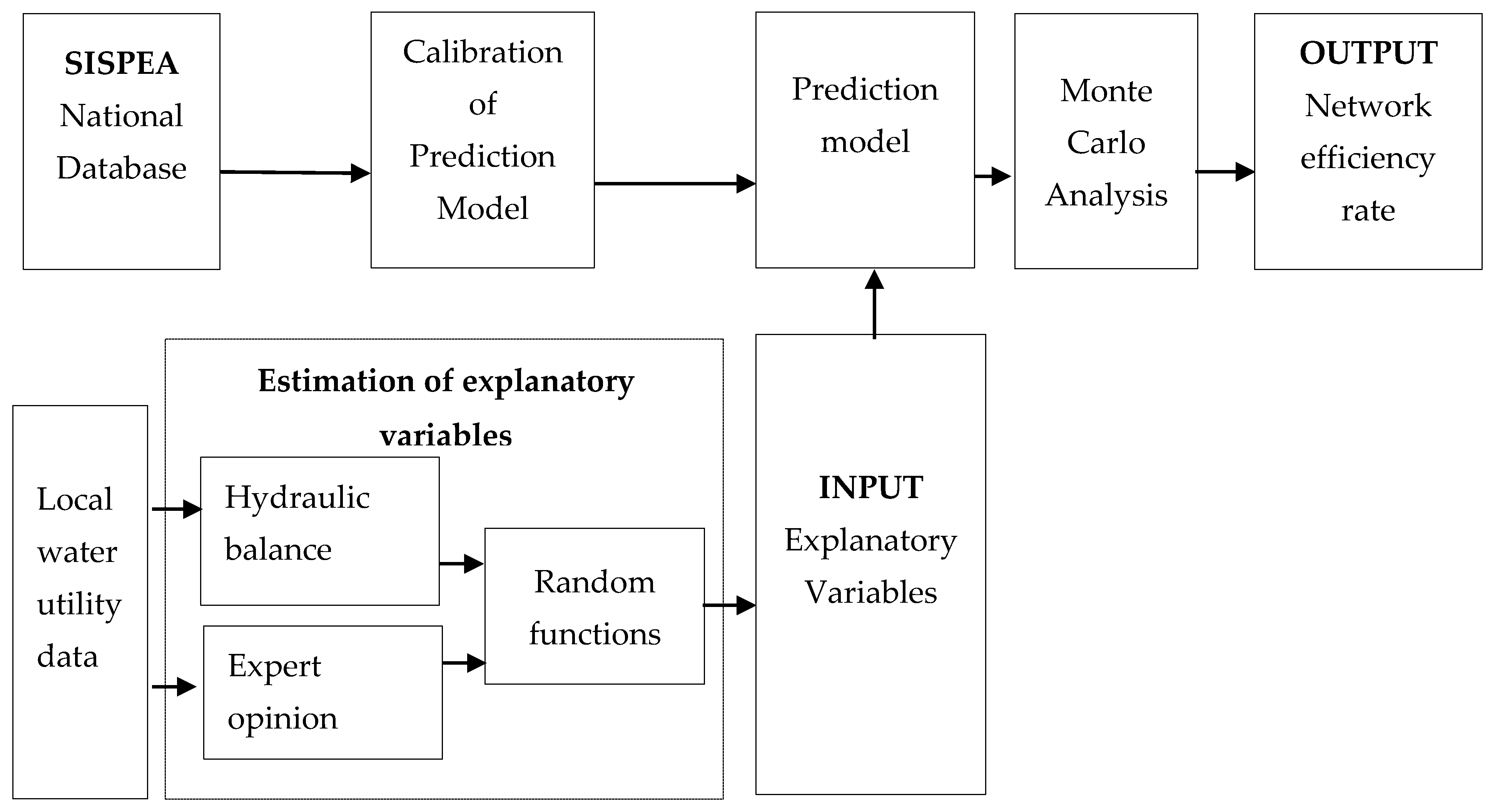
2. Materials and Methods

The approach developed in this research aims to help the water utility manager to decrease NRW, even in the context of non-existence of data, to monitor water loss. The use of machine learning methods requires the availability of important data set to ensure the training of prediction model. Our model establishes causal relationships between efficiency rate—output—and local network data—input—according to two complementary steps: (i) the calibration of predicting model based on national data and (ii) estimation of explanatory variables—input—model data based on specific mathematical functions and expert opinions. Figure 1 shows an overview of the developed model and its main steps.

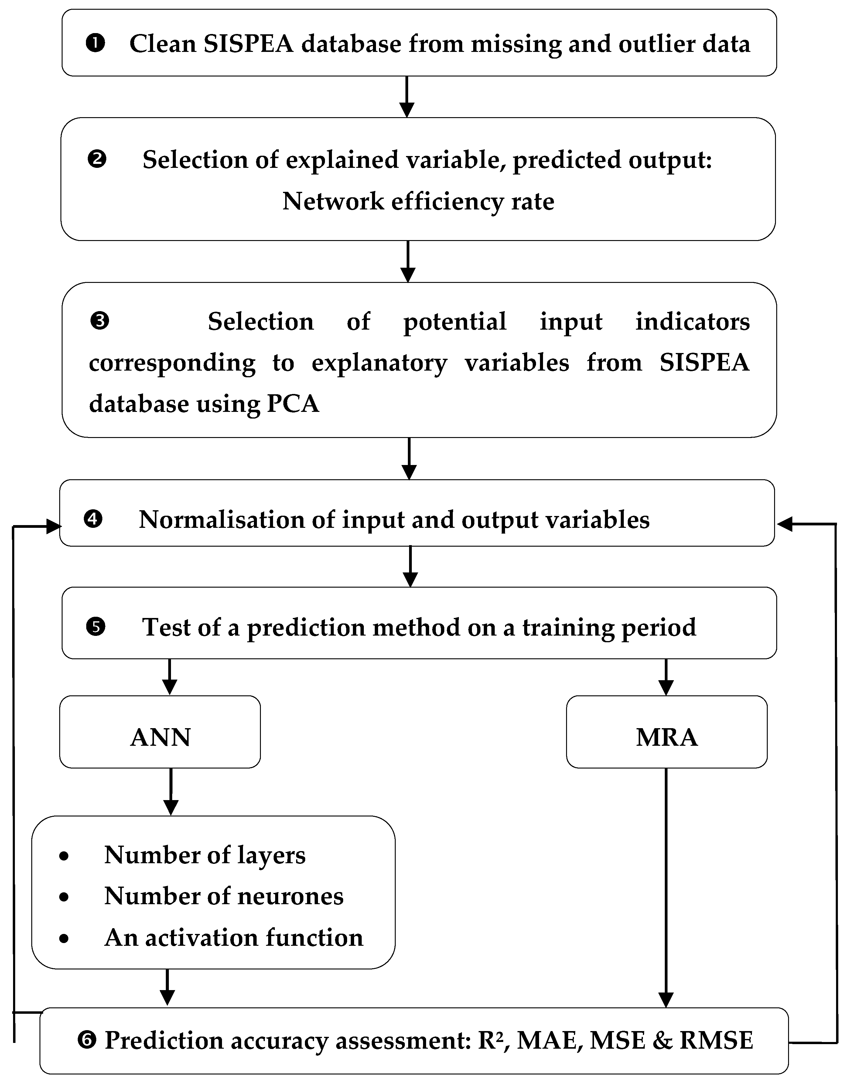
2.1. Calibration of the Prediction Model: National Analysis

In order to counter the unavailability of local network data, we used “SISPEA”, a French information system for water and wastewater services used for monitoring and benchmarking water and waste water utilities. The information system is a national database that contains 29 mandatory performance indicators collected over a ten-year period (2006–2016) covering financial, technical, management and quality of service domains. Gathered data are representative of 47% of French water utilities which supply 79% of the French population. We assume that it is possible to establish a causal model between the efficiency rate and other performance indicators using ANN or MRA. The fitting of the prediction model will not be done on local data of a specific water utility, but rather, on a national dataset. Figure 2 details the main steps for model calibration.

The replicability of the developed approach in other contexts seems possible for many reasons. The existence of benchmarking initiatives at national, regional or international levels is reported in [19], who cite as an example, the European Benchmarking cooperation (EBC) or the international benchmarking network for water and sanitation utilities (IBNET) supported by the world banks. These networks assume the existence of specific information systems containing performance indicators at local or national scales. A non-exhaustive list of national benchmarking systems similar to SISPEA is established by [20]. The water services information systems (VEETI) in Finland, the DANVA benchmarking system in Denmark, the system bedreVA in Norway, the system VENLA in Finland.

Because French performance indicators and those gathered from the cited information systems are derived from International Water Association (IWA) indicators, there is a high similarity in terms of potential explanatory variables useable for calibrating a prediction model. This aspect confirms the possible reuse or adaptation of our model in other contexts or countries. The use of national data is due to the unavailability of enough historical data at local scale. The developed model is not limited by the fact that data are gathered at local or national scale, but by the availability of enough explanatory variables that fit the prediction model. It is easily replicable in contexts where local data are available. The adaptability of the developed approach constitutes a real added value for water utility management to support decisions.

2.1.1. Predicted Output: The Water Efficiency Rate

In our case, the explained variable that has to be predicted is the water efficiency rate (WER). The French mandatory definition of this indicator is given by the Equation (1):

$$\mathrm{WER}=\left(\frac{\begin{array}{c}\mathrm{Billed}\mathrm{metered}\mathrm{domestic}\mathrm{consumption}+\mathrm{Billed}\mathrm{metered}\mathrm{non}\mathrm{domestic}\mathrm{consumption}+\\ \mathrm{unbilled}\mathrm{metered}\mathrm{consumption}+\mathrm{billed}\mathrm{exported}\mathrm{water}\end{array}}{\mathrm{metered}\mathrm{produced}\mathrm{water}+\mathrm{metered}\mathrm{imported}\mathrm{water}}\right)\times 100\%$$

(1)

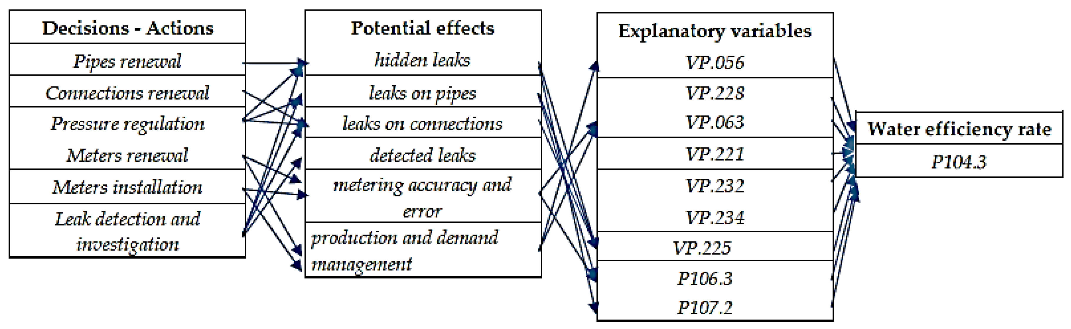
2.1.2. Selection of Explanatory Variables

The analysis of mandatory indicators allows us to define potential indicators considered as explanatory variables for network efficiency. Principal Component Analysis (PCA) is conducted on a set of variables pre-selected by the expert. The analysis of our own values and accumulative variability of the principal components indicates if it is required to add or remove variables. The set of potential correlated explanatory variables corresponds to the variables forming the first dimension (factor) of PCA. The process of selection is stopped when the variability of the first dimension reaches its maximum value.

The

Table 1. Potential explanatory variables for efficiency rate.

Leakage Management Actions	SISPEA Code	Explanatory Variables—Indicators	Explained Variable—Target
Metering and metering error	VP.056	Number of users	Network efficiency rate (P104.3)
	VP.228	Linear density of users
	VP.063	Billed metered domestic consumption
	VP.221	Volume of unmetered consumption
	VP.232	Billed metered consumption
	VP.234	Volume produced + Volume imported
Leakage and water losses	VP.225	Average network efficiency rate over 3 last years
	P106.3	Linear leakage index on distribution mains
Pipes renewal	P107.2	Average renewal rate of water mains over the 5 last years

lists potential explanatory variables.

The identification of explanatory variables is relevant for the prediction of efficiency rate, but not enough to help the water utility manager to support decisions. Thus, it is necessary to highlight relationships between potential decisions or actions and selected explanatory variables in order to assess their consequences in terms of performance and costs. At this stage of the research, we consider the following potential operation or investment decisions to support: leak detection and leaks reparation, connections renewal, pipes renewal. Pressure management and actions to improve metering accuracy (DMA, meters renewal and installation) are not addressed by the current work. We assume that a potential policy is a mix of decisions or actions. Figure 3 illustrates relationships between potential decisions, explanatory variables and water efficiency rate.

The benefit of decisions can be estimated by the improvement of the water efficiency rate. The total cost (C_Tot) of decisions is obtained by the sum-up of operation expenditures (OPEX) and capital expenditures (CAPEX). The simulation of policy alternatives is ensured by the decision maker and not generated automatically. The Equation (2) calculates the total annual cost (C_Tot) of decisions or a policy:

$$C_{Tot}=CAPEX+OPEX$$

(2)

By considering potential operation decisions, OPEX can be calculated by the Equation (3) that involves the following variables:

• C_rep: unit cost of a leak reparation in € per unit.
• C_det: unit cost in € per km
• n_c: number of leaks on connections per year
• n_p: number of leaks on pipes per year
• n_d: number of leaks detected by leak detection

$$OPEX=\left(n_p+n_c+n_d\right)\times C_{rep}+l_{det}\times C_{det}$$

(3)

By considering potential asset management decisions of pipes or connections renewal, CAPEX can be calculated by Equation (4):

$$CAPEX=r_c\times n_c\times C_{con}+r_p\times l_{net}\times C_p$$

(4)

where:

• C_con: unit cost of a connection renewal in € per unit
• C_p: unit cost of pipe renewal in € per km
• l_net: length of the network
• r_c: annual connections renewal rate in percentage per year
• r_p: annual renewal rate in percentage of length renewed per year

We assume that cost data are available in the IS of the water utility or can be estimated. In order to analyze cost and benefit of decisions, we propose using a specific metric Gain-Effort, GE defined in [21]. It assesses the elasticity of the gain in relation to achieved effort; in our case, we calculate the elasticity of the performance in relation to the cost. The metric can be obtained by dividing the relative variation of performance by the relative variation of total cost calculated by Equation (5):

$$GE=\frac{\frac{\Delta P}{P}}{\frac{\Delta C_{Tot}}{C_{Tot}}}$$

(5)

The GE assesses the variation of performance due to a variation of expenditures. The value of (1/GE) measures the required effort in terms of expenditures per unit of performance improvement.

2.1.3. Normalization of Variables

The explained and explanatory variables should be normalized in order to remove bias due to scale and unit differences. It seems that learning machines models are sensitive to variables difference of magnitude, which is the reason why it is recommended to transform them before [9,10,11,12,13,14,15,16,17]. The z-score normalization is frequently used in learning models [7], and the new scale is defined as in Equation (6):

$$X_{scaled}=\frac{X_i-mean\left(X\right)}{{\sigma }_X}$$

(6)

This transformation places the values around 0, so the transformed variables have an average of 0. Furthermore, by dividing by the standard deviation, the distribution of the variable is standard and has a standard deviation of 1.

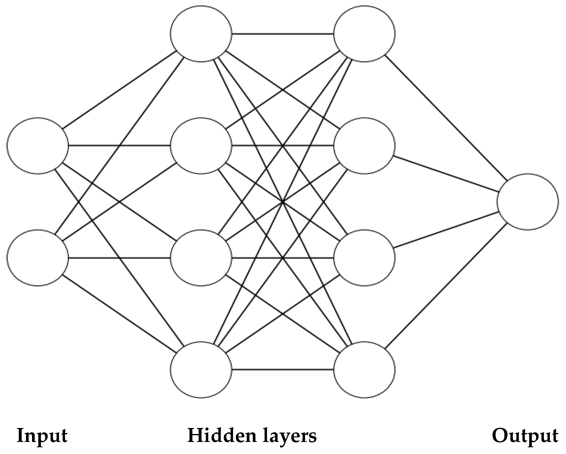
2.1.4. Prediction Method: Multiple Regression Analysis (MRA) and Artificial Neural Network (ANN)

Multiple regression analysis (MRA) establishes a correlation between explained and explanatory variables using Equation (7):

Y = βX + ε₀

(7)

with:

• Y: vector of explained variables (output);
• X: vector of explanatory variables (input);
• β: variables coefficients;
• ε₀: vector of error estimation.

Variables are not directly used in their current values but transformed according to a specific metric. The best fit is obtained using the ordinary least squares method. This method consists in minimizing the sum of the squares of the differences between observed and predicted variables. The predicted value may be biased in case of insufficient data availability; a high robustness model requires a large amount of input data. In order to validate the regression results, two tests are commonly performed [11] to reject the following assumptions:

• The assumption that no variables are explanatory for the regression. This hypothesis is tested with an F-test. The F value must exceed a critical value in order to reject the hypothesis.
• The assumption that the true coefficient of an explanatory variable is zero. This hypothesis is tested by computing the p-value. If p-value is greater than 0.05, the hypothesis is rejected and therefore the variable has an explanatory effect.

A multiple linear regression model is compared to the ANN which belongs to artificial learning methods, to predict non-revenue water ratio [6]. Obtained results show a low correlation between the predicted value and the true value. As an improvement, authors use a multiple nonlinear regression model which improves their prediction significantly. According to [18,22], ANN represents an efficient tool to deal with complex causal relationships. The developed approach implements multiple layers perceptron (MLP). MLP contains a first layer with all explanatory variables, a layer with the output variables and one or more hidden layers between the input and output layers. There is no clear agreement on the number of hidden layers and neurons to use. The number of hidden neurons depends very strongly on available input data and the complexity of the problem to solve. In case the of insufficient input data, hidden layers and neurons will not provide good training of the neural network. On the other hand, too many hidden layers and neurons can lead to overfitting. An over-fitted model provides good results on training tests but is not accurate for prediction. Only tests of several combinations of hidden layers with various numbers of neurons can improve the training of ANN and can improve the accuracy of prediction. According to their experiment feedback, the authors of [6,7] advise setting the number of hidden neuron layers equal to twice the number of explanatory variables. Figure 4 illustrates an ANN configuration.

Each neuron is defined by a transfer function f, a set of $w_i$ for each output of the previous layer and a bias $b_0$. A neuron computes the following function: $f({\displaystyle \sum }(w_i{x}_i+b_0)$ with $x_i$ the input received from neuron i of the previous layer.

Note that x is the input data of the neuron. The list of transfer functions widely used is as follows [12]:

• The logistic function that is often preferred with Equation (8):

  $$f\left(x\right)=\frac{1}{1+e^{-x}}$$

  (8)
• The hyperbolic tangent function (tanh) that can sometimes lead to better results than the logistic function [15] with Equation (8):

  $$f\left(x\right)=\frac{2}{1+e^{-2x}}-1$$

  (9)
• The rectified linear unit function (ReLU), the expression of which is given by Equation (10):

  $$f\left(x\right)=\{0 for x<0;x for x\ge 0\}$$

  (10)
• The identity function, the expression of which is defined by Equation (11):

  $$f\left(x\right)=x$$

  (11)

In order to determine the precision of the model and to be able to compare different prediction models, the observed variable value and the predicted value are compared.

Many indicators can be computed [9]. One of them is the coefficient of determination R² that is calculated by Equation (12):

$$R^2=1-{\displaystyle \sum }_{i=1}^n\frac{{\left(y_i-\widehat{y_i}\right)}^2}{{\left(y_i-mean\left(y\right)\right)}^2}$$

(12)

where:

• n the number of input values;
• $y_i$ the value of input i;
• $\widehat{y_i} the corresponding predicted value$
• $mean\left(y\right)$ the mean of the input values.

The coefficient of determination is ranged between 0 and 1. If its value is close to 1, it means that the prediction model is correctly fitted. Another indicator seems relevant because it assesses the average error between observed and predicted value. The mean absolute error (MAE) is computed by Equation (13):

$$MAE=\frac{1}{n}{\displaystyle \sum }_{i=1}^n(|y_i-\widehat{y_i}|)$$

(13)

The mean absolute error is positive and represents the mean prediction error of the model, the accuracy of prediction increases when the value of MAE is close to 0. The mean square error MSE is also useful to assess the accuracy of the prediction; it is computed according to Equation (14):

$$MSE=\frac{1}{n}{\displaystyle \sum }_{i=1}^n{\left(y_i-\widehat{y_i}\right)}^2$$

(14)

Like the mean absolute error, the mean square error is positive and a value close to 0 is targeted. This indicator penalizes larger errors more heavily than the average absolute error. The last accuracy indicator is the square root of the mean square error RMSE, the expression of which is given by Equation (15):

$$RMSE=\sqrt{\frac{1}{n}{\displaystyle \sum }_{i=1}^n{\left(y_i-\widehat{y_i}\right)}^2}$$

(15)

This indicator is frequently used to measure the differences between the values predicted by a model and the observed values [23]. The square root of the mean square error is positive and a value close to 0 is targeted.

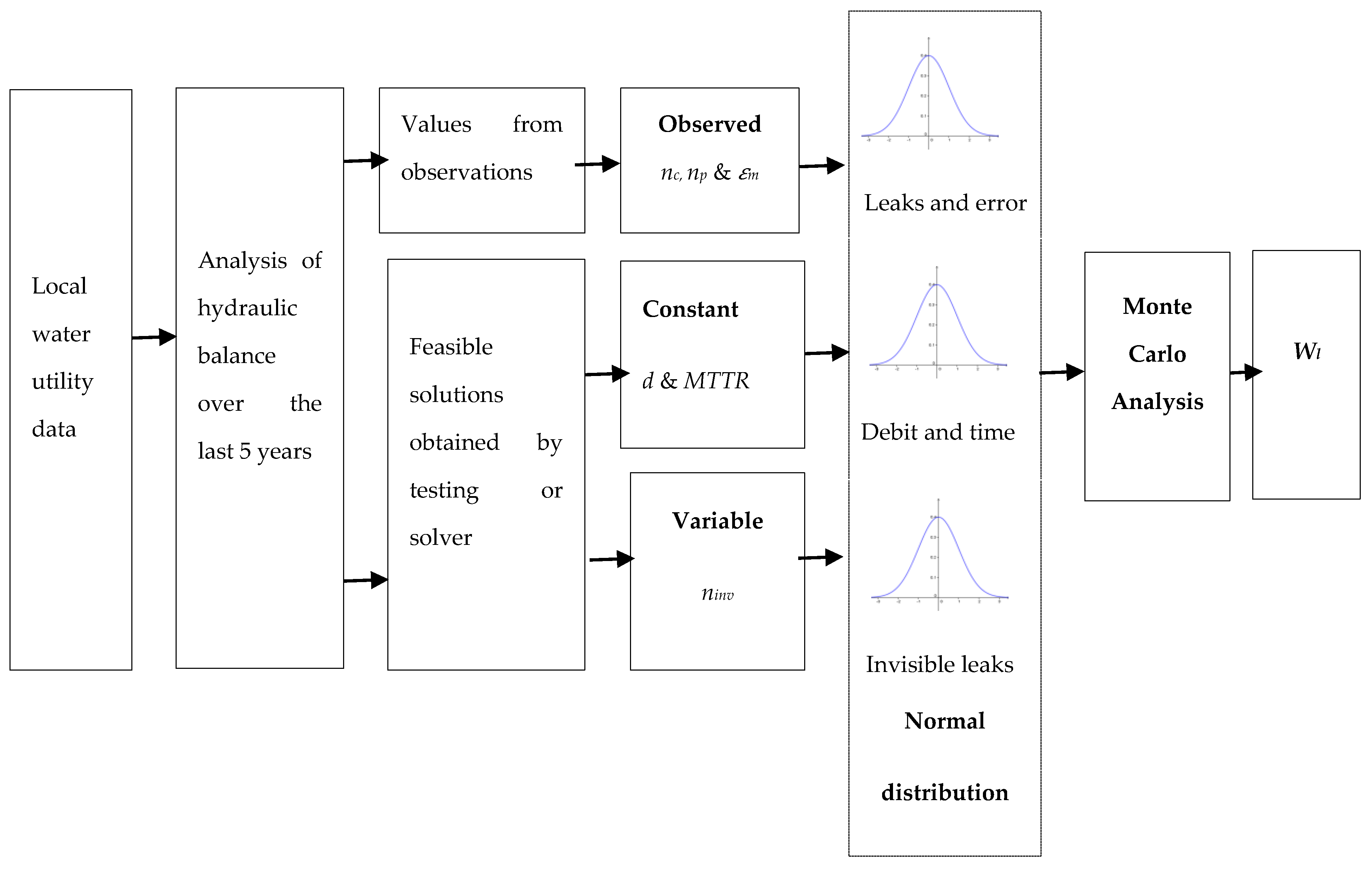
2.2. Estimation of Explanatory Variables

The second step of our approach aims at estimating explanatory variables from existing utility data using dedicated mathematical functions and expert opinion. In the absence of reliable data or a large window of observation data, Monte Carlo analysis is implemented to deal with estimation uncertainty. This section illustrates methods for estimating explanatory variables listed in Table 1. Two methods are used: (i) random generation using distribution function and (ii) mathematical function

2.2.1. Random Generation

A set of explanatory variables is estimated, based on random generation ensured by uniform discrete or continuous distribution probability functions. Expert opinion or water utility expertise defines the range of variation of values depending on the trend of the variable and the context of the utility. The trend could be estimated by an absolute or relative value of increase or decrease of a reference value: average value, last observation or expectation. The variable is generated randomly between the upper (U) and lower (L) limits with a probability equals to 1/(U − L).

Table 2. Estimation of explanatory variables using random functions.

SISPEA Code	Explanatory Variables—Indicators	Function	Type	Unit	Range of Variation
VP.056	Number of users	Uniform	Discrete	#	Depends on past trend and potential evolution of the demand and water uses
VP.228	Linear density of users	Ratio	Continuous	#/km
VP.063	Billed metered domestic consumption	Uniform	Continuous	m3	Depends on past trend and potential evolution of the demand and water uses
VP.221	Volume of unmetered consumption	Uniform	Continuous	m3	Depends on the improvement or decrease of metering accuracy, actions in terms of leakage management or meters renewal or installation.
VP.232	Billed metered consumption	Uniform	Continuous	m3	Depends on past trend and potential evolution of the demand and water uses
VP.234	Volume produced + Volume imported	Uniform	Continuous	m3	Depends on production capacities, demand evolution and water importation evolution
VP.225	Average network efficiency rate over 3 last years	Mean ratio	Continuous	%	Observation over the last 3 years
P107.2	Average renewal rate of water mains over the 5 last years	Mean ratio	Continuous	%	Observation over the last 5 years

details the distribution functions to be used for generating explanatory variables and their potential range of variation.

2.2.2. Hydraulic Balance

The calculation of the linear leakage index (LI) on distribution mains is calculated by Equation (16):

$$LI=\frac{W_l}{Network length}$$

(16)

In order to assess this variable, it is required to assess the potential annual water losses W_l. A specific mathematical function for water loss prediction based on annual hydraulic balance is defined according to the following hypotheses:

• Real losses are due to visible leaks observed on pipes, connections and other hydraulic components. Hidden leaks are detected with leaks detection techniques.
• Debit for visible leak is higher than for hidden leak
• Renewal, maintenance and reparation actions contribute to water loss reduction
• Metering error should be considered in the hydraulic balance because it artificially increases water losses.
• Water losses depend highly on hidden leaks that should be estimated
• Mean time to repair (MTTR) is considered as one of the key parameters for water loss reduction.

The volume of distributed water for a year (t) can be estimated based on a hydraulic balance on the entire network by Equation (17) as follow:

$$W_d\left(t\right)=W_b\left(t\right)+W_l\left(t\right)+W_{aut}\left(t\right)+W_{non aut}\left(t\right)+W_{ser}\left(t\right)\pm {\epsilon }_m\left(t\right)$$

(17)

We can deduce the estimation of annual losses according to Equation (18):

$$W_l\left(t\right)=W_d\left(t\right)-\left[W_b\left(t\right)+W_{aut}\left(t\right)+W_{non aut}\left(t\right)+W_{ser}\left(t\right)\pm {\epsilon }_m\left(t\right)\right]$$

(18)

Based on the hypothesis that real losses are generated by visible and hidden leaks, the theoretical estimation of annual water losses is given by Equation (19):

$$\begin{array}{cc}\hfill W_l\left(t\right)={\epsilon }_m\left(t\right)+& n_p\left(t\right)\times MTT{R}_{vl}\left(t\right)\times d_p\left(t\right)+n_c\left(t\right)\times MTT{R}_{vl}\left(t\right)\times d_c\left(t\right)+n_{inv}\left(t\right)\hfill \\ & \times MTT{R}_{inv}\left(t\right)\times d\left(t\right)-r_d\left(t\right)\times L_{net}\left(t\right)\times MTT{R}_{inv}\left(t\right)\times d\left(t\right)-r_p\left(t\right)\hfill \\ & \times L_{net}\left(t\right)\times r_b\left(t\right)\times MTT{R}_{vl}\left(t\right)\times d_p\left(t\right)-r_c\left(t\right)\times n_c\left(t\right)\times MTT{R}_{vl}\left(t\right)\times d_c\left(t\right)\hfill \end{array}$$

(19)

Equation (19) can be simplified as follows:

$$\begin{array}{cc}\hfill W_l\left(t\right)={\epsilon }_m\left(t\right)+& MTT{R}_{vl}\left(t\right)\hfill \\ & \times [n_p\left(t\right)\times d_p\left(t\right)+n_c\left(t\right)\times d_c\left(t\right)-r_p\left(t\right)\times L_{net}\left(t\right)\times d_p\left(t\right)\times r_b\left(t\right)-r_c\left(t\right)\hfill \\ & \times n_c\left(t\right)\times d_c\left(t\right)]+MTT{R}_{inv}\left(t\right)\times [n_{inv}\left(t\right)\times d\left(t\right)-r_d\left(t\right)\times L_{net}\left(t\right)\times d\left(t\right)]\hfill \end{array}$$

(20)

Equation (20) clearly shows that the volume of water losses depends on the mean time to repair, leakage rate and the number of leaks. The metering error ε_m(t) could be estimated from available data or defined according to manager expertise. The use of this equation in practice seems difficult because data for the debit, number of leaks, time to repair are hard to collect.

Table 3. List of the variables and the symbols.

Symbol	Definition of the Variable	Unit
Wd	Annual volume of distributed water	m3
Wb	Annual volume of billed water	m3
Wl	Annual volume of water loss (real)	m3
Wp	Annual volume of produced water	m3
Wimp	Annual volume of imported water	m3
Wexp	Annual volume of exported water	m3
Waut	Annual volume of authorized unbilled consumption	m3
Wser	Annual Volume of unbilled water for service	m3
Wnon aut	Annual volume of unauthorized water	m3
np	Number of breaks/leaks on pipes per year	#
nc	Number of breaks/leaks on connections per year	#
Lnet	Network length (without length of connections)	#
nc	Number of connections
ninv	Number of hidden leaks per year	#
dp	Average debit for a leak on pipe	L/s
dc	Average debit for leak on connection	L/s
d	Average debit for hidden leak	L/s
MTTRvl	Mean Time to repair visible leak	S
MTTRinv	Mean time to repair hidden leaks	S
rd	Efficiency ratio of leak detection (number of detected leaks per km)	#/km of investigation
rp	Water pipes annual renewal rate	%
rc	Connections annual renewal rate	%
rb	Pipes breakage rate	#/km
Crep	Cost of pipe or connection reparation	€ per reparation
Cp	Cost of pipe renewal	€/km
Cc	Cost of connection reparation	€ per reparation
Cdet	Cost of leak detection	€ /km of leak detection
εm	Metering error in percentage or in volume	% or m3

lists and defines mentioned variables and symbols.

To overcome the obstacle of the non-existence of information, Equation (20) is used to estimate the mean and standard deviation of leakage rate (debits), the number of leaks and repair time for both pipes and connections over an observation period of 5 years. These values represent a set of feasible solutions that satisfy the annual hydraulic balance for each year of the observation period.

Conversely, we assume that the average values of debit d and time to repair MTTR are constant over the observation period. The number of hidden leaks n_inv(t) changes from year to year to allow the equilibrium of the hydraulic balance. The number of visible breaks and leaks on pipes and connections are supposed to be available as local data from the water utility. To involve the uncertainty of estimation, a Monte Carlo analysis is implemented using Equation (20), where a set of parameters and variables of the equation are randomly generated as shown in Figure 5. In absence of data concerning the characteristics of leaks, normal distribution functions are used to randomly generate debit, the number of leaks and time to repair. The achievement of this analysis provides a potential range of values for parameters of Equation (20) that makes the estimation of water losses possible for prediction purposes. Figure 5 illustrates the required steps to estimate annual water losses.

The combination of the two methods presented in this section allows for estimating explanatory variables, in order to provide input data for the prediction of the network efficiency rate. The next section details the implementation of the developed approach on a real case study.

3. Case Study

As shown in previous sections, the implementation of the developed model requires the availability of an important set of data in order to fit the prediction model. In the French context, the use of the machine learning approach is very difficult at local scale because most of the water utilities’ GIS do not contain enough observation data concerning leaks and water losses. The national SISPEA database constitutes a viable alternative, as its data show the performance of French water and wastewater utilities. Several mandatory indicators are provided by utilities and centralized in a SISPEA, which allows for performance analysis and benchmarking.

SISPEA gathered data for more than 12,832 water utilities between 2006 and 2016. After the analysis of database items, several missing data were observed. Only 14,000 (2000 per year) observations concerning the nine inputs potential explanatory variables listed in Table 1 are exploitable over the period between 2010 and 2016. Data were split into two samples. A total of 70% of the data is used to calibrate the model and the remaining 30% is used to validate it.

The analysis of dataset shows that variables are incommensurables, which is why their normalization is preconized. We use Z-score normalization as defined by Equation (6).

Table 4. Characteristics of exploitable variables over the observation period (2010–2016).

Variables	Mean	Standard Deviation
VP.056	5.28 × 105	3.26 × 106
VP.228	8.33 × 105	4.50 × 106
VP.063	5.36 × 104	4.43 × 105
VP.221	2.49 × 102	7.07 × 103
VP.232	4.00 × 103	1.66 × 104
VP.234	3.08 × 10	2.16 × 10
VP.225	5.82 × 105	3.51 × 106
P106.3	0.35 × 10	0.48 × 10

indicates values of mean and standard deviation for exploitable variables.

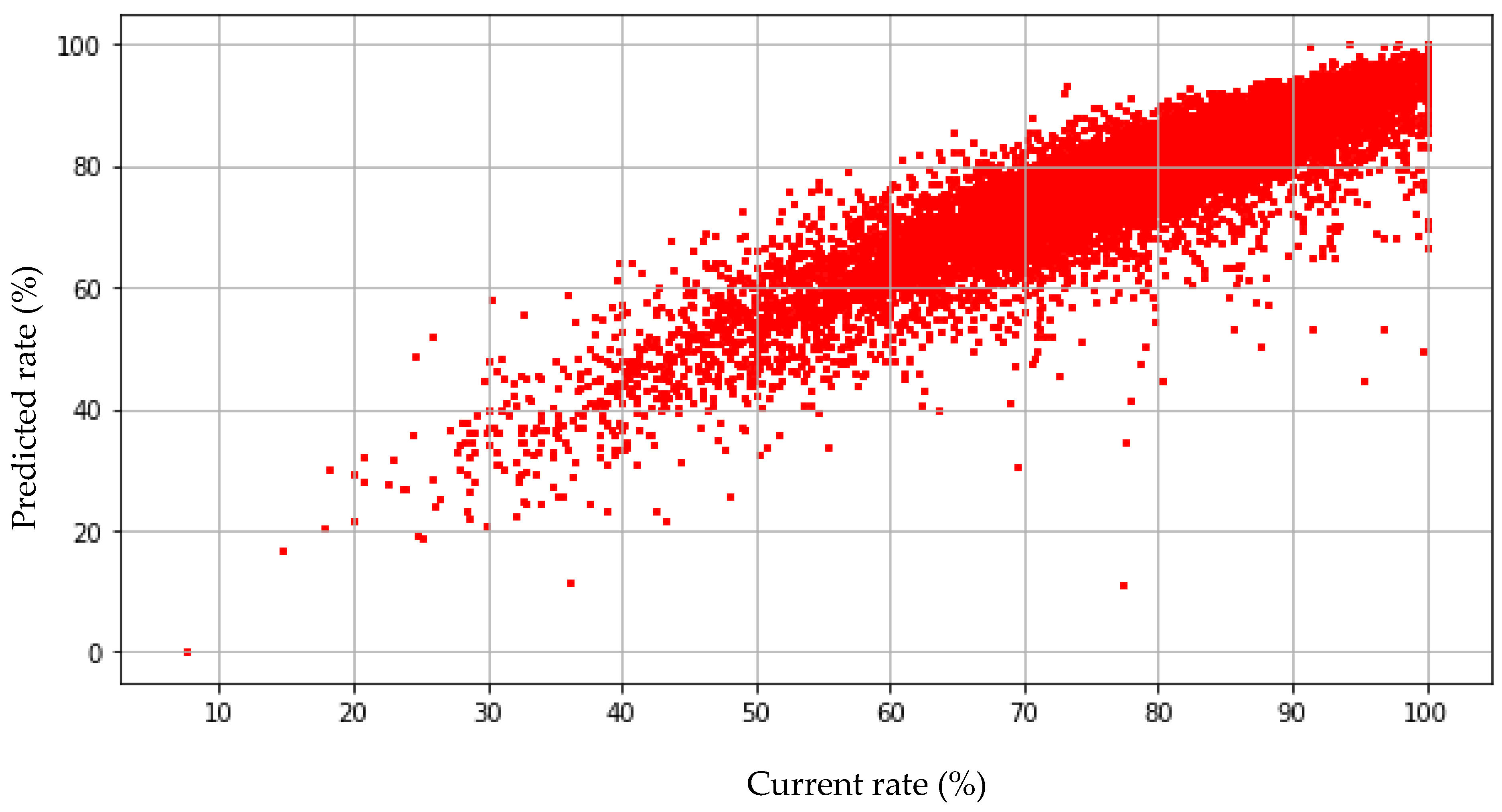
3.1. Multiple Regression Analysis

PCA and MRA are applied to the set of normalized variables to calibrate the prediction model. A total of 9 variables are retained as explanatory variables because of their level of statistical significance.

In order to assess the capacity of MRA to predict the efficiency ratio, we compare predicted values and observed values retained for validation. Each dot in Figure 4 represents predicted or observed values. In case of perfect match, only one dot is observed that indicates that prediction is accurate. In that case, the distribution of dots is concentrated around the first bisector. Figure 3 shows a significant difference between predicted and observed values.

The analysis of Figure 6 is confirmed by

Table 5. Assessment of the accuracy of prediction in case of MRA.

Accuracy Indicator	MAE	MSE	R2
MRA	3.921	31.101	0.805

. The accuracy of the prediction obtained with MRA could be improved, as the R² value is around 0.8 and the error values are high.

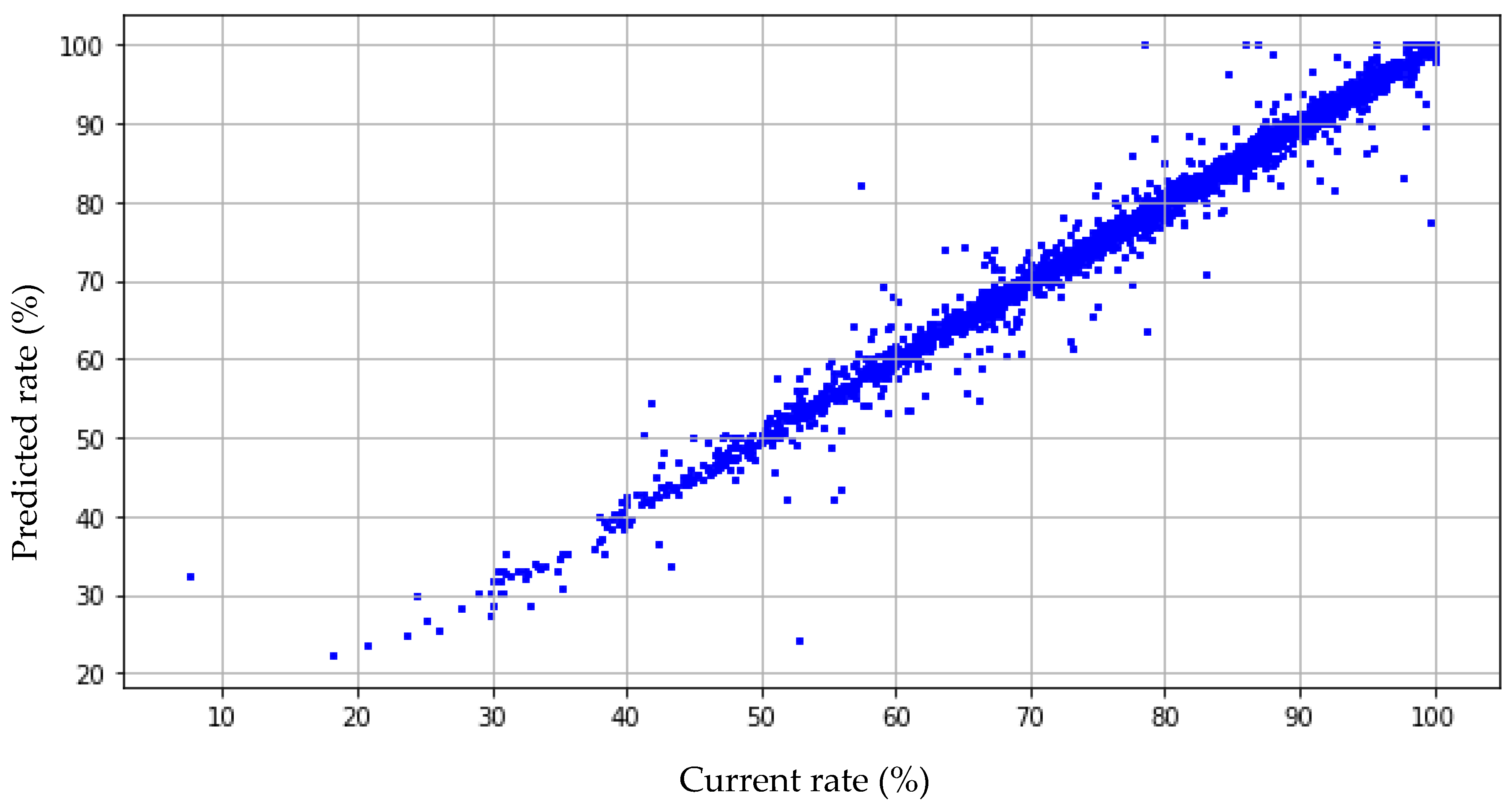
3.2. Artificial Neural Network Calibration

The same dataset and input variables are used to calibrate the prediction model using ANN. Data are shared with the same proportions into 2 samples, one for training and one for prediction. The training of the ANN requires more steps. In fact, many parameters should be fitted in order to improve the accuracy of the prediction and define the structure parameters of the ANN. Among these parameters it is necessary to (i) determine the number of neurons, (ii) determine the number of hidden layers and (iii) define the type of activation function. Several simulations are implemented with combinations of values for cited parameters.

Table 6. Influence of the activation function on the prediction accuracy.

Activation Function	Hidden Layer	Number of Neurons	MAE	MSE	R2
Identity	Single layer	18	4.038	32.771	0.798
Rectified linear unit	Single layer	18	2.035	9.470	0.942
Hyperbolic tangent	Single layer	18	1.312	6.879	0.958
Logistic	Single layer	18	1.382	6.695	0.959

asses the influence of the chosen activation function on the prediction accuracy. Four different types of activation functions are tested for a fixed number of neurons equal to 18. The accuracy is assessed using the following indicators: MAE, MSE, and R² values.

Table 6 clearly shows that the accuracy of prediction is significantly improved when the hyperbolic tangent function or logistic function are selected. While these results cannot be generalized, they seem relevant to our case study. Based on this observation, other simulations have been performed to determine the best combination between the number of neurons and the number of hidden layers.

According to the previous result, the logistic function improves the accuracy of prediction. It also offers the advantage of being easy to fit, in comparison to the hyperbolic function. By choosing a logistic function as an activation function, we assess the influence of the configuration of the ANN on the accuracy of the prediction. Several configurations have been tested by modifying the number of layers and the number of neurons per layer as shown in

Table 7. Tested values for artificial neural network (ANN) structure parameters.

Hidden Layer	Number of Neurons	MAE	MSE	R2
Single layer	9	1.689	7.719	0.952
Single layer	18	1.382	6.695	0.959
Single layer	36	1.215	5.764	0.965
Single layer	72	1.269	6.738	0.959
Multiple layer	(9, 9)	1.200	4.334	0.973
Multiple layer	(18, 18)	1.027	3.575	0.978
Multiple layer	(36, 36)	0.775	3.025	0.981
Multiple layer	(72, 72)	0.810	4.614	0.972
Multiple layer	(18, 9)	0.910	3.320	0.980
Multiple layer	(9, 18)	1.116	4.314	0.973
Multiple layer	(36, 18)	0.808	3.322	0.980
Multiple layer	(18, 36)	0.848	5.120	0.968
Multiple layer	(72, 36)	0.859	6.691	0.980
Multiple layer	(36, 72)	0.835	5.268	0.968

; completed tests clearly indicate the existence of a relationship between the number of layers, the number of neurons, and prediction accuracy. The range of variation in the R² value remains low (between 0.952 and 0.981), but conversely, the MAE value decreases from 1.689 in the case of nine neurons with a single layer to 0.775 with two hidden layers with 36 neurons each. Even if the analysis is not exhaustive, it allows for defining the best configuration of the ANN in order to improve the prediction. According to Table 6, the retained configuration of the ANN is obtained for the minimum value of MAE and R². The ANN to be used for prediction will be composed of two hidden layers of 36 each. Figure 7 is drawn in order to assess the capacity of the prediction model to match the observation on the validation period. Dots seem more concentrated around the first bisector, indicating a higher accuracy of prediction obtained by ANN than with MRA.

The implementation of MRA and ANN shows in our case, the relevance of the choice of the prediction method.

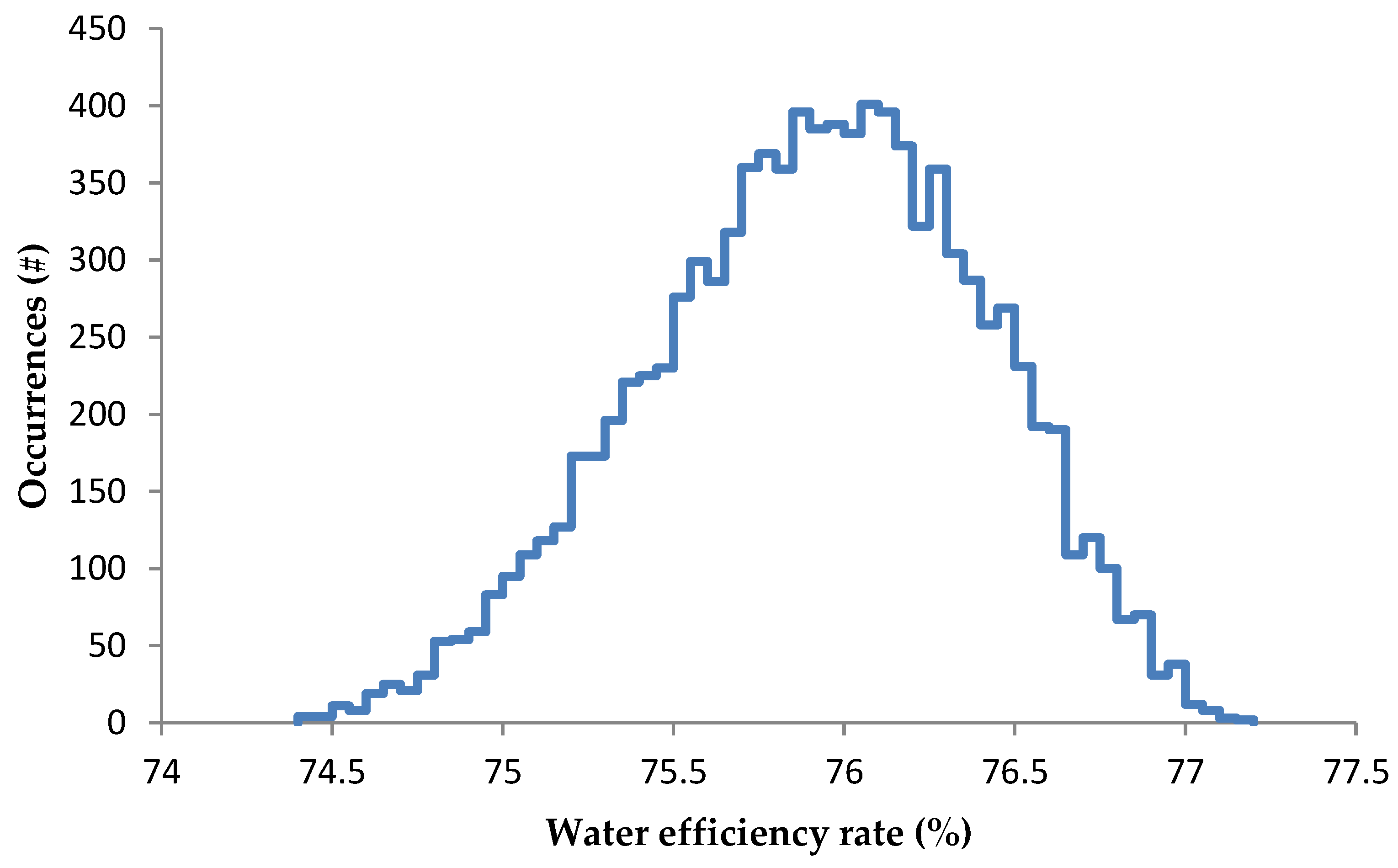
3.3. Estimation of Explanatory Variables

The previous sections detail the first step of our model, by calibrating a prediction model based on a national database. The following section details how the second step of our model is implemented in order to estimate explanatory variables from a specific water utility—local data—in order to estimate the efficiency ratio. In 2016, the selected utility delivered around 0.7 million m³ of water for more than 6400 consumers using 82 km of water distribution network. A significant improvement in the water efficiency ratio was observed. The ratio increased from 65.9% in 2010 to 76.6% in 2016.

In order to check if models calibrated using a national dataset are also accurate using a local data set, we implement MRA and ANN on the observed local explanatory variables for the past period between 2010 and 2016.

Table 8. Observed and predicted values for efficiency ratio between 2010 and 2016.

Year	Observed (%)	Predicted-MRA (%)	Predicted-ANN (%)
2010	65.9	63.0	65.7
2011	63.2	61.7	62.4
2012	61.4	60.2	60.7
2013	75.0	67.6	75.1
2014	75.1	71.2	75.1
2015	76.9	75.6	76.8
2016	76.6	76.5	76.6

compares predicted and observed values of the water efficiency ratio.

Table 8 indicates that prediction model using MRA and ANN fitted on the national dataset gives an accurate prediction on the local dataset. However, ANN seems more accurate; the analysis of accuracy indicators given by

Table 9. Accuracy indicators for prediction model implemented to local data.

Accuracy Indicators	MRA	ANN
R2	0.745	0.991
MAE	2.185	0.407
MSE	10.030	0.339
RMSE	3.167	0.582

shows it clearly. The MAE value is very low and R² is close to one for the prediction achieved with ANN.

The estimation of explanatory variables for the year (N + 1 = 2016) based on the past trend requires expert opinions and the use of local data for hydraulic balance. As detailed by Equation (16) and illustrated by Figure 3, the assessment of water losses needs to estimate the number of leaks breaks on pipes, the number of leaks on connections, the average value for MTTR and leak debits.

Table 10. Variables estimation for water losses and LI assessment at year (N + 1).

Variables	Year N	Past Trend	Expert Opinion	Estimation
np	10	+20%	[−20%; +20%]	Uniform distribution (Discrete)
nc	18	−6%	[−15%; +20%]	Uniform distribution (Discrete)
dp	5 m3/h	+1%	[−10%; +10%]	Uniform distribution (Continuous)
dc	3 m3/h	−5%	[−10%; +10%]	Uniform distribution (Continuous)
MTTRvl	24 h	−43%	[−50%; −10%]	Uniform distribution (Continuous)

indicates several expert opinions to estimate the explanatory variable LI at the year (N + 1) using Monte Carlo analysis.

The same approach was implemented to estimate the rest of the explanatory variables based on expert opinion and Monte Carlo analysis.

The use of both ANN prediction model and Monte Carlo simulation on the variables contained in

Table 11. Estimation of explanatory variables for efficiency ratio prediction.

Leakage Management Actions	SISPEA Code	Explanatory Variables—Indicators	Average	Expert Opinion	Estimation
Metering and metering error	VP.056	Number of users	6377	[0%; +1%]	Uniform distribution function
	VP.228	Linear density of users	78.53	[−5%; 0%]	Uniform distribution function
	VP.063	Billed metered domestic consumption	660,831	[−10%; −5%]	Uniform distribution function
	VP.221	Volume of unmetered consumption	1511	[−20%; −15%]	Uniform distribution function
	VP.232	Billed metered consumption	687,259	[0%; 10%]	Uniform distribution function
	VP.234	Volume produced + Volume imported	1,047,827	[0%; +20%]	Uniform distribution function
Leakage and water losses	VP.225	Average network efficiency rate over the last 3 years.	75.67%		Average value
	P106.3	Linear leakage index on distribution mains	7.64	[−10%; −5%]	Uniform distribution function
Pipes renewal	P107.2	Average renewal rate of water mains over the last 5 years	0.71%	[−100%; −90%]	Uniform distribution function

allows us to predict the value of the water efficiency ratio for the year 2016 based on past trends and observed local data. For 10,000 simulations, the water efficiency ratio value is ranged between 74.41% and 77.18% with an average efficiency value equal to 75.91%. Figure 8 illustrates the result of the simulations.

The interval of predicted values involves the observed value for the year 2016 equal to 75.73%. The developed model seems accurate and consistent. The developed approach offers to the decision maker the possibility to simulate alternatives and assess their cost and benefit. An alternative is preferred according to its comparison to the actual practices of the water utility in terms of operation and asset management, defined by: leak detection investigations of 100% of the network, renewal pipes rate of 0.7% and 2% of connections renewal rate per year. These actions cost annually 560,503 € shared between 70% of CAPEX and 30% of OPEX. The current practices define a baseline policy.

Table 12. Cost and benefit of leak detection increase.

Decisions			Cost and Benefit
Leak Detection	Pipe Renewal	Connections Renewal Rate	Efficiency Rate (Benefit)	Total Cost (€)	CAPEX	OPEX	Cost Variation	Performance Variation	GE
100%	0.70%	2%	75.73%	560,503	70%	30%
150%	0.70%	2%	76.93%	614,907	64%	36%	+10%	+1.58%	16.33%
200%	0.70%	2%	78.13%	669,311	59%	41%	+19%	+3.17%	16.33%
250%	0.70%	2%	79.92%	723,715	54%	46%	+29%	+5.53%	19.00%
300%	0.70%	2%	80.52%	778,119	50%	50%	+39%	+6.33%	16.29%

illustrates how the developed approach can drive decisions. The results show the cost and benefit of potential alternatives based on the increase of the length of network proven by leak detection. We assume that detected hidden leaks are repaired. We notice that the increase of leak detection and OPEX are positively correlated to the water efficiency rate. As illustrated, when the network is totally checked 3 times a year (300% of the length), the efficiency rate increases from 75.73% to 80.52%. This decision implies an increase of expenditures by 39% in comparison with the baseline decision and has an influence on the performance, as the efficiency rate increases by 6.33%. This is confirmed by the GE value that indicates that when expenditures are enhanced by 100%, the expected increase of performance will be ranged between 16% and 20%. We can also interpret (1/GE) that indicates that the improvement of performance by 1% requires an increase of expenditures ranged between 5% and 6%.

Table 13. Cost and benefit of pipes renewal rate increase.

Decisions			Cost and Benefit
Leak Detection	Pipe Renewal	Connections Renewal Rate	Efficiency Rate (Benefit)	Total Cost (€)	CAPEX	OPEX	Cost Variation	Performance Variation	GE
100%	0.70%	2%	75.73%	560,503	70%	30%
100%	1.05%	2%	75.74%	645,683	74%	26%	+15%	0%	0%
100%	1.40%	2%	75.74%	730,864	77%	23%	+30%	0%	0%
100%	1.75%	2%	75.75%	816,044	79%	21%	+46%	0%	0%
100%	2.10%	2%	75.75%	901,224	81%	19%	+61%	0%	0%

contains results of the simulation of decisions based on the increase of pipes renewal rate as asset management decisions. We observe that the increase of pipes renewal rate increases total Cost (+61%) and CAPEX without any incidence on the performance, the GE is equal to 0.

Table 14. Cost and benefit of connections renewal rate increase.

Decisions			Cost and Benefit
Leak Detection	Pipe Renewal	Connections Renewal Rate	Efficiency Rate (Benefit)	Total Cost (€)	CAPEX	OPEX	Cost Variation	Performance Variation	GE
100%	0.70%	2%	75.73%	560,503	70%	30%
100%	0.70%	3%	75.80%	670,173	75%	25%	+20%	+0.09%	0.47%
100%	0.70%	4%	75.86%	781,837	79%	21%	+39%	+0.17%	0.43%
100%	0.70%	5%	75.92%	892,504	81%	19%	+59%	+0.25%	0.42%
100%	0.70%	6%	75.98%	1,003,171	83%	17%	+79%	+0.33%	0.41%

shows cost and benefit of decisions based on the increase of connections renewal rate as asset management decisions. The performance improvement is a little sensitive to the variation of connections renewal rate; the increase of expenditures by +79% implies an increase of performance only by 0.33%. This is confirmed by the GE value, that indicates that even if expenditures are enhanced by 100%, the expected increase of performance will range between 0.41% and 0.47%. The interpretation of (1/GE) indicates that the improvement of performance by 1% requires an increase of expenditures ranged between 200 % and 240%.

Simulations of various decisions show that our approach constitutes an added value for testing alternatives and assessing their costs and benefits. This aims at defining the most appropriate decisions in relation to water efficiency improvement. Even if obtained results are ad-hoc, the proposed approach allows for identifying the type of decisions between operation and asset management decisions. It clearly indicates to the decision maker if it is preferable to enhance CAPEX or OPEX in relation with the water efficiency performance. In the case of the considered utility, it is recommended to better investigate the network rather than to renew it, particularly when the goal is to increase water efficiency. This result is correct in the short term and does not consider a whole life analysis of the asset and positive effects of asset renewal in the long term. This aspect is important, because here, only one performance indicator is considered. The automatic generation and assessment of feasible and compromised alternatives is not addressed in the current work; it constitutes a very interesting challenge and a way to improve our approach.

4. Conclusions

The prediction model developed in this paper offers a real alternative solution for estimating the trend of water utility performance by exploiting local and national datasets. The developed model establishes a causal relationship between planned actions, expected actions, and their trends (decrease or improvement) and the level of performance assessed in our case by the water efficiency ratio. It constitutes a real tool for prospective purposes concerning water loss management and network operation improvement by linking the set of explanatory variables to decisions alternatives on the one hand, and to the water efficiency rate on the other hand. This is the heart of our model; expert opinion is guided by past trend, expected actions in terms of maintenance, investment and leak detection in order to improve performance with minimum OPEX and CAPEX.

The developed approach is able to estimate OPEX and CAPEX of actions and their benefit in terms of performance improvement. This renders possible to test a mix of decisions between the improvement of the network operation and the network condition by renewing assets. It appears from our case study that the improvement of water efficiency rate required more investigations and leak detection than asset renewal. This result cannot be generalized, but can constitute an interesting driver for networks with high level of performance and where the marginal improvement costs less if operation actions are planned rather than investment actions.

The range of variation of explanatory variables is sensitive both to planned and expected actions. The practical implementation of the developed model requires a diagnosis of the water utility IS. The availability of enough data at local scale allows to calibrate the prediction model using ANN or MRA based on preconized explanatory variables. In the case of absence of local data, it is necessary to calibrate the model based on a national IS. The unavailability of data at a water utility scale renders the use of machine learning inconsistent or impossible; our two-step prediction model counters this problem by using a national database and adapting it to the local scale. For both situations, the water utility manager will be able to assess costs and benefit (performance) of actions as shown in the case study in order to support decisions.

Obtained results from the implementation of the developed model reflect those found in the literature review, notably which ANNs appear to be more accurate than MRA. Another consistent result concerns the relevance of the selection of the activation function and the configuration of the ANN in order to improve the prediction accuracy. Several tests of the number of neurons and hidden layers increase the accuracy of prediction. The main novelty of our work consists of adopting a general prediction model calibrated on a national trend to a local context using specific explanatory variables. The use of expert analysis and Monte Carlo simulations compensate the unavailability of local data (water loss, debit, MTTR, hidden leaks) and permits us to involve uncertainty in the prediction of the water efficiency ratio. Prediction results are concordant with observations, which indicate that the prediction model could help water utility managers to estimate performance trends according to the context evolution.

The use of high-level explanatory variables driven from national information systems can contribute to an easy replicability of the approach in other contexts. In fact, the existence of benchmarking initiatives around the world suppose the existence of dedicated information system that enables to assess, to gather and to benchmark similar performance indicators of those contained in the French information system “SISPEA”. Adaptions will be required depending on data availability and the variables to explain. The use of ANNs and MRA as predictive models in other contexts or for other variables seems to be possible and has to be tested in a future research.

For instance, the generation of alternatives and decisions are done manually; the use of dedicated approach for alternatives exploration should be investigated. Other possible improvement concerns the consideration of multiple indicators and how it could affect the calibration of the prediction model. The use of multi-objective genetic algorithm for the generation and the assessment of alternatives could be relevant. The availability of local data could improve accuracy and may improve the causal relationship; further research should address all mentioned aspects and test the robustness of the model and how it is possible to generalize the developed approach and results. At this stage, the initial results are encouraging.

References

1. Adedeji, K.; Hamam, Y.; Abe, B.; Abu-Mahfouz, A. Leakage Detection and Estimation Algorithm for Loss Reduction in Water Piping Networks. Water 2017, 9, 773. [Google Scholar] [CrossRef]
2. Colombo, A.; Karney, B. Energy and Costs of Leaky Pipes: Toward Comprehensive Picture. J. Water Resour. Plan. Manag. 2002, 128, 441–450. [Google Scholar] [CrossRef]
3. Salvetti, M. The network efficiency rate: A key performance indicator for water services asset management? In Proceedings of the 7th IWA International Conference on Efficient Use and Management of Water (Efficient 2013), Paris, France, 22–25 October 2013. [Google Scholar]
4. Candelieri, A.; Archetti, F.; Messina, E. Improving leakage management in urban water distribution networks through data analytics and hydraulic simulation. WIT Trans. Ecol. Environ. 2013, 171, 107–117. [Google Scholar] [Green Version]
5. Xin, K.; Tao, T.; Lu, Y.; Xiong, X.; Li, F. Apparent Losses Analysis in District Metered Areas of Water Distribution Systems. Water Resour. Manag. 2014, 28, 683–696. [Google Scholar] [CrossRef]
6. Jang, D.; Choi, G. Estimation of Non-Revenue Water Ratio Using MRA and ANN in Water Distribution Networks. Water 2017, 10, 2. [Google Scholar] [CrossRef]
7. Jang, D.; Park, H.; Choi, G. Estimation of Leakage Ratio Using Principal Component Analysis and Artificial Neural Network in Water Distribution Systems. Sustainability 2018, 10, 750. [Google Scholar] [CrossRef]
8. Shirzad, A.; Tabesh, M.; Farmani, R. A comparison between performance of support vector regression and artificial neural network in prediction of pipe burst rate in water distribution networks. KSCE J. Civ. Eng. 2014, 18, 941–948. [Google Scholar] [CrossRef]
9. Jafar, R.; Shahrour, I.; Juran, I. Application of Artificial Neural Networks (ANN) to model the failure of urban water mains. Math. Comput. Model. 2010, 51, 1170–1180. [Google Scholar] [CrossRef]
10. Tabesh, M.; Soltani, J.; Farmani, R.; Savic, D. Assessing pipe failure rate and mechanical reliability of water distribution networks using data-driven modeling. J. Hydroinform. 2009, 11, 1–17. [Google Scholar] [CrossRef] [Green Version]
11. Nishiyama, M.J. Forecasting Water Main Failures in the City of Kingston Using Artificial Neural Networks; Department of Civil Engineering, Queen’s University: Kingston, ON, Canada, 2013; 105p. [Google Scholar]
12. Kutylowska, M. Prediction of failure frequency of water-pipe network in the selected city. Period. Polytech. Civ. Eng. 2017, 61, 548–553. [Google Scholar] [CrossRef]
13. Kamiński, K.; Kamiński, W.; Mizerski, T. Application of Artificial Neural Networks to the Technical Condition Assessment of Water Supply Systems. Ecol. Chem. Eng. S 2017, 24, 31–40. [Google Scholar] [CrossRef] [Green Version]
14. Rojek, I.; Studziński, J. Comparison of different types of neuronal nets for failures location within water-supply networks. Maint. Reliab. 2014, 16, 42–47. [Google Scholar]
15. Gholami, V.; Sebghati, M.; Yousefi, Z. Integration of artificial neural network and geographic information system applications in simulating groundwater quality. Environ. Health Eng. Manag. J. 2016, 3, 173–182. [Google Scholar] [CrossRef] [Green Version]
16. Giustolisi, O.; Simeone, V. Optimal design of artificial neural networks by a multi-objective strategy: Groundwater level predictions. Hydrol. Sci. J. 2006, 51, 502–523. [Google Scholar] [CrossRef]
17. Rahmati, S.H.; Haddad, O.B.; Sedghi, H. and Babazadeh, H. A comparison of anfis, ann, arma & multivariable regression methods for urban water-consumption forecasting, considering impacts of climate change: A case study on Tehran mega city. Indian J. Sci. Res. 2014, 7, 870–880. [Google Scholar]
18. Makaya, E.; Hensel, O. Modelling flow dynamics in water distribution networks using artificial neural networks—A leakage detection technique. Int. J. Eng. Sci. Technol. 2016, 7, 33–43. [Google Scholar] [CrossRef]
19. Berg, S.; Padowski, J.C. Overview of Water Utility Benchmarking Methodologies: From Indicators to Incentives; Public Utility Research Center, University of Florida: Gainesville, FL, USA, 2007; Available online: http://warrington.ufl.edu/centers/purc/purcdocs/papers/0712_Berg_Overview_of_Water.pdf (accessed on September 2018).
20. Osmo, T.S. Performance benchmarking in Nordic water utilities. Procedia Econ. Financ. 2015, 21, 399–406. [Google Scholar] [CrossRef]
21. Nafi, A.; Tcheng, J.; Beau, P. Comprehensive Methodology for Overall Performance Assessment of Water Utilities. Water Resour. Manag. 2015, 29, 5429–5450. [Google Scholar] [CrossRef]
22. Hornik, K.; Stinchcombe, M.; White, H. Multilayer feedforward networks are universal approximators. Neural Netw. 1989, 2, 359–366. [Google Scholar] [CrossRef]
23. Hsu, K.; Gupta, H.V.; Sorooshian, S. Artificial Neural Network Modeling of the Rainfall-Runoff Process. Water Resour. Res. 1995, 31, 2517–2530. [Google Scholar] [CrossRef]
Figure 1. Main steps of the developed model.
Water 10 01443 g001
Figure 2. Calibration of the prediction model using a national database.
Water 10 01443 g002
Figure 3. Potential relationships between decisions and the water efficiency rate.
Water 10 01443 g003
Figure 4. Artificial Neural Network configuration.
Water 10 01443 g004
Figure 5. Steps for annual water losses estimation.
Water 10 01443 g005
Figure 6. Comparison of predicted and observed values—case of multiple regression analysis (MRA).
Water 10 01443 g006
Figure 7. Comparison of predicted and observed values—case of ANN.
Water 10 01443 g007
Figure 8. Monte Carlo simulation results for prediction of efficiency rate.
Water 10 01443 g008